12 bioprocess control - iste · 12 bioprocess control ... temperature, ph, etc. 1.3. a schematic...
TRANSCRIPT
12 Bioprocess Control
and control, enabling real-time optimization of the bioprocess operation. Theseapproaches are obviously complementary to one another. This book discusses thematter within the context of the final approach.
1.2. Specific problems of bioprocess control
Over the past several decades, biotechnological processes have been increasinglyused industrially, which is attributed to several reasons (improvement of profitabilityand quality in production industries, new legislative standards in processing indus-tries, etc.). The problems arising from this industrialization are generally the sameas those encountered in any processing industry and we face, in the field of biopro-cessing, almost all of the problems that are being tackled in automatic control. Thus,system requirements for supervision, control and monitoring of the processes in orderto optimize operation or detect malfunctions are on the increase. However, in reality,very few installations are provided with such systems. Two principal reasons explainthis situation:
– first of all, biological processes are complex processes involving living organ-isms whose characteristics are, by nature, very difficult to apprehend. In fact, themodeling of these systems faces two major difficulties. On the one hand, lack ofreproducibility of experiments and inaccuracy of measurements result not only in oneor several difficulties related to selection of model structure but also in difficultiesrelated to the concepts of structural and practical identifiability at the time of iden-tification of a set of given parameters. On the other hand, difficulties also occur atthe time of the validation phase of these models whose sets of parameters could haveprecisely evolved over course of time. These variations can be the consequence ofmetabolic changes of biomass or even genetic modifications that could not be fore-seen and observed from a macroscopic point of view;
– the second major difficulty is the almost systematic absence of sensors providingaccess to measurements necessary to know the internal functioning of biological pro-cesses. The majority of the key variables associated with these systems (concentrationof biomass, substrates and products) can be measured only using analyzers on a labo-ratory scale – where they exist – which are generally very expensive and often requireheavy and expensive maintenance. Thus, the majority of the control strategies usedin industries are very often limited to indirect control of fermentation processes bycontrol loops of the environmental variables such as dissolved oxygen concentration,temperature, pH, etc.
1.3. A schematic view of monitoring and control of a bioprocess
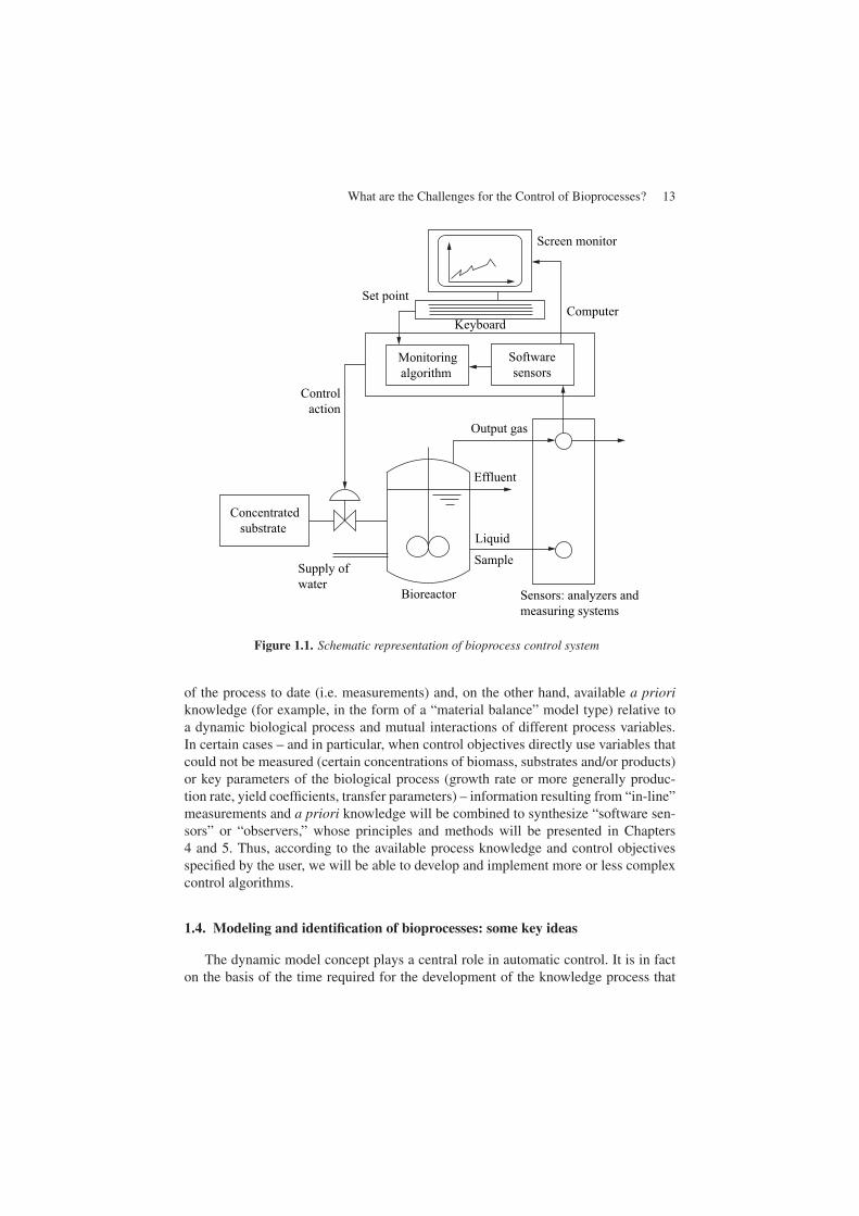
Use of a computer to monitor and control a biological process is representedschematically in Figure 1.1. In the situation outlined, the actuator is the feed rateof the reactor. Its value is the output of the control algorithm, which uses the infor-mation of the available process. This information regroups, on the one hand, the state
What are the Challenges for the Control of Bioprocesses? 13
Sample
Effluent
Screen monitor
ComputerSet point
Keyboard
Monitoringalgorithm
Softwaresensors
Controlaction
Output gas
Concentratedsubstrate
Supply ofwater
Liquid
Bioreactor Sensors: analyzers andmeasuring systems
of the process to date (i.e. measurements) and, on the other hand, available a prioriknowledge (for example, in the form of a “material balance” model type) relative toa dynamic biological process and mutual interactions of different process variables.In certain cases – and in particular, when control objectives directly use variables thatcould not be measured (certain concentrations of biomass, substrates and/or products)or key parameters of the biological process (growth rate or more generally produc-tion rate, yield coefficients, transfer parameters) – information resulting from “in-line”measurements and a priori knowledge will be combined to synthesize “software sen-sors” or “observers,” whose principles and methods will be presented in Chapters4 and 5. Thus, according to the available process knowledge and control objectivesspecified by the user, we will be able to develop and implement more or less complexcontrol algorithms.
1.4. Modeling and identification of bioprocesses: some key ideas
The dynamic model concept plays a central role in automatic control. It is in facton the basis of the time required for the development of the knowledge process that
Figure 1.1. Schematic representation of bioprocess control system
14 Bioprocess Control
the total design, analysis and implementation of monitoring and control methods arecarried out. Within the framework of bioprocesses, the most natural way to determinethe models that will enable the characterization of the process dynamics is to considerthe material balance (and possibly energy) of major components of the process. It isthis approach that we will consider in this work (although certain elements of hybrid
in the chapter on modeling). One of the important aspects of the balance models is thatthey consist of two types of terms representing, respectively, conversion (i.e. kinetics
substrates in terms of biomass and products) and the dynamics of transport (whichregroups transit of matter within the process in solid, liquid or gaseous form and thetransfer phenomena between phases). These models have various properties, whichcan prove to be interesting for the design of monitoring and control algorithms forbioprocesses, and which will, thus, be reviewed in Chapter 2. Moreover, we will intro-duce in Chapter 4 on state observers a state transformation that makes it possible towrite part of the bioprocess equations in a form independent of the process kinetics.This transformation is largely related to the concept of reaction invariants, which arewell known in the literature in chemistry and chemical engineering.
An important stage of modeling consists not only of choosing a model suitableand appropriate for describing the bioprocess dynamics studied but also of calibratingthe parameters of this model. This stage is far from being understood and thereforeno solution has been obtained, given the complexity of models as well as the (fre-quent) lack of sufficiently numerous and reliable experimental data. Chapter 3 willattempt to introduce the problem of identification of the parameters of the models ofthe bioprocess (in dealing with questions of structural and practical identifiability aswell as experiment design for its identification) and suitable methods to carry out thisidentification.
1.5. Software sensors: tools for bioprocess monitoring
As noted above, sometimes many important variables of the process are not acces-sible to be measured online. Similarly, many parameters remain unclear and/or arelikely to vary with time. There is, thus, a fundamental need to develop a model, whichmakes it possible to carry out a real-time follow-up of variables and key parameters ofthe bioprocess. Thus, Chapters 4 and 5 will attempt, respectively, to develop softwaretools to rebuild the evolution of these parameters and variables in the course of time.Insofar as their design gives reliable values to these parameters and variables, they playthe role of sensors and will thus be called “software sensors”. The material is dividedbetween the two chapters on the basis of distinction between state variables (i.e. pri-marily, component concentrations) whose evolution in time is described by differen-tial equations and parameters (kinetic, conversion and transfer parameters), which areeither the functions of process variables (as is typically the case for kinetic parameters
modeling, which combines balance equations and neural networks, will be addressed
of various biochemical reactions of the process and conversion yields of various
What are the Challenges for the Control of Bioprocesses? 15
such as specific growth rates) or constants (output parameters, transfer parameters)1.For state variables, we will proceed with the design of “software sensors” called stateobservers (Chapter 4), whereas for estimating the unknown or unclear parametersonline, parameter estimators will be used (Chapter 5). Due to space considerations,Chapter 5 will deal exclusively with the estimation of kinetic parameters, which provesto be a more crucial problem to be solved. However, the methods which are developedare also applicable to other parameters.
1.6.
profile compatible with an optimal operating condition. Chapter 6 will attempt todevelop the basic concepts of automatic control applied to bioprocesses, particularly
portional and integral actions. We can also initiate certain control methods specificto bioprocesses. The following chapter will concentrate on the development of moresophisticated control methods with the objective of guaranteeing the best possiblebioprocess operation while accounting, in particular, for disturbances and modelinguncertainties. Emphasis will be placed, particularly, on optimal control and adaptivecontrol methods based on the balance model as developed in the chapter on model-ing. The objective is clearly to obtain control laws, which seek the best compromisebetween what is well known in bioprocess dynamics (for example, the reaction schemeand the material balance) and what is less understood (for example, the kinetics).
1.7. Bioprocess monitoring: the central issue
With the exception of real-time monitoring of state variables and parameters, therehas been little consideration of bioprocess monitoring. In particular, how to managebioprocesses with respect to various operation problems, which are about malfunction-ing or broken down sensors, actuators (valves, pumps, agitators, etc.), or even morebasically malfunction of the bioprocess itself, if it starts to deviate from the nomi-nal state (let us not forget that the process implements living organisms, which canpossibly undergo certain, at least partial, transformations or changes, which are likelyto bring the process to a different state from that expected). This issue is obviouslyimportant and cannot be ignored if we wish to guarantee a good real time processoperation. This problem calls for all the process information (which is obtained frommodeling, physical and software sensors or control). This will be covered in the finalchapter.
1. The models used in practice are often so simplified with respect to reality that these param-eters can “apparently” undergo certain variations with time. However, it is important to notethat these variations are nothing but a reflection of the inaccuracy or inadequacy of the selectedmodel.
Bioprocess control: basic concepts and advanced control
operation, less susceptible to various disturbances, close to a certain state or desiredAn important aspect of bioprocess control is to lay down a stable real time
the concepts of control and setpoint tracking, feedback, feedforward control and pro-
68 Bioprocess Control
for its robustness with respect to the local minima, its ease of implementation and itsreasonable convergence speed [PRE 86, SCH 98, VAN 96].
Global minimization
The global minimization methods can be roughly classified into two groups[SCH 98]. The first group comprises purely deterministic methods, such as thegridding method. It consists of evaluating the objective function for a large numberof points predefined over a grid covering the parameter space. If there is a sufficientnumber of function evaluations, there are chances of attaining the minima. Thismethod is not very effective, unless it is improved by refining the grid after a series ofevaluations.
The second group of global methods can be called random probing methods, asrandom decisions are included in the procedure for attaining the optimum. Amongthem, the adaptive methods take into account the information obtained during the pre-ceding evaluations. For one method (simulated annealing [PRE 86]), the idea is thatthe search will not always be toward a possible solution (which could just be a localminimum), but may be, from time to time, along another direction. This method can beviewed as preceding the popular methods such as genetic algorithms (GA) [GOL 89].These algorithms commence with an initial population of prospective solutions (some-what similar to the edges in the Simplex method) sampled in a random manner in theparameter space. In genetic algorithms, new prospective solutions are obtained byimitating the process of biological evolution of cross breeding, mutation and selectionamong the parameter “populations”. The definition of the parameters of the algorithmitself is crucial for correct implementation.
3.6. A case study: identification of parameters for a process modeled for anaero-bic digestion
The anaerobic digestion model (2.16)–(2.29) formed the subject matter for a sys-tematic study to identify parameters on the basis of a fixed bed reactor of LBE - INRAat Narbonne (see [BER 01, BER 00] for a more detailed study). This case study isremarkable in view of many aspects. Firstly, the identification of parameters is riddledwith traps that are typical for biological systems: the process is very complex (numer-ous bacterial populations participate in the process; they can have different behaviorsdepending on the operating conditions). There are no direct measurements for each ofthe acidogenic and methanogenic bacterial populations and in general, a limited num-ber of process variables are accessible. The process is slow and can be destabilizedeasily by the accumulation of fatty acids. These characteristics have significant conse-quences for the selected model. The model cannot be very complex lest it should turnout to be non-identifiable, whereas the simplified modeling hypotheses can have animpact on its capacity to predict the dynamics of the process. The choice of the struc-ture is therefore a critical stage in view of the fact that the model should necessarilycontain elements that are essential for the process dynamics.
Identification of Bioprocess Models 69
Moreover, the identification itself contains original elements with respect to therest of the chapter. Constraints on the process have led us to conceive an experimentalplan, not on the basis of the above techniques but motivated by concern for coveringas wide a range of operating conditions as possible, while at the same time limiting theduration (here necessarily long) of the experiments as much as possible. In addition,the structure of the reaction system models enables us to separate the parameters intothree classes (yield coefficients, kinetic parameters and transfer parameters) and tocarry out the identification of each class of parameters in a distinct manner.
In this case study, emphasis is laid on parameter estimation using linear regression.Having said this, it will be prudent to draw attention to the fact that this approach can-not turn out to be optimum from a statistical point of view insofar as the statistical con-ditions on the variables used in the linear regression could not be completely fulfilledin order to enable an estimation that might be statistically accurate and sufficientlyreliable. In general, care must be taken during the interpretation of the estimated val-ues of parameters and their standard deviation. Furthermore, these parameter valuesgiven by linear regression were suggested to be used as initial values of an estimationon the basis of the nonlinear model. However, such an estimation has not turned outto be useful in the present case.
3.6.1. The model
Let us once again proceed from the equations developed in Chapter 2. A variantof these was considered as here we are dealing with a fixed bed reactor, where thebacteria are fixed on supports. Thus, formally there is no dilution term in the balanceequations. However, on the other hand, it was noted that a portion of the biomasswas detached: it was hypothesized that the rate of detachment was proportional to therate of dilution, represented by coefficient α. Under these conditions, the model isrewritten as follows:
dX1
dt= μ1X1 − αDX1 (3.43)
dX2
dt= μ2X2 − αDX2 (3.44)
dS1
dt= D(S1in − S1)− k1μ1X1 (3.45)
dS2
dt= D(S2in − S2) + k2μ1X1 − k3μ2X2 (3.46)
dZ
dt= D(Zin − Z) (3.47)
dC
dt= D(Cin − C)− qC + k4μ1X1 + k5μ2X2 (3.48)
70 Bioprocess Control
qC = kLa(C − S2 − Z −KHPC) (3.49)
PC =φ−√φ2 − 4KHPT (C + S2 − Z)
2KH(3.50)
φ = C + S2 − Z +KHPT +k6
kLaμ2X2 (3.51)
qM = k6μ2X2 (3.52)
pH = −log10(Kb
C − Z + S2
Z − S2
)(3.53)
In addition, growth models were chosen, one Monod model for acidogenesis andone Haldane model for methanization:
μ1 =μmax 1S1
KS1 + S1, μ2 =
μ0S2
KS2 + S2 + S22/KI2
(3.54)
In the absence of systematic rule, this choice was dictated by a desire to havekinetic models that are sufficiently simple, coherent with those normally used foranaerobic digestion, but also capable of highlighting the potential instability of theprocess in the presence of the accumulation of volatile fatty acids (explaining thechoice of the Haldane model for μ2).
Knowing that Kb and KH are known chemical and physical constants (Kb = 6.510−7 mol/l, KH = 16 mmol/l/atm), we note that the model contains 13 parameters tobe identified. In addition, the variables available for the measurement are the dilutionrate D, the inlet concentrations, S1in, S2in, Zin, Cin, the gas flow rates qC , qM , theconcentrations S1, S2, Z, C, and the pH.
3.6.2. Experiment design
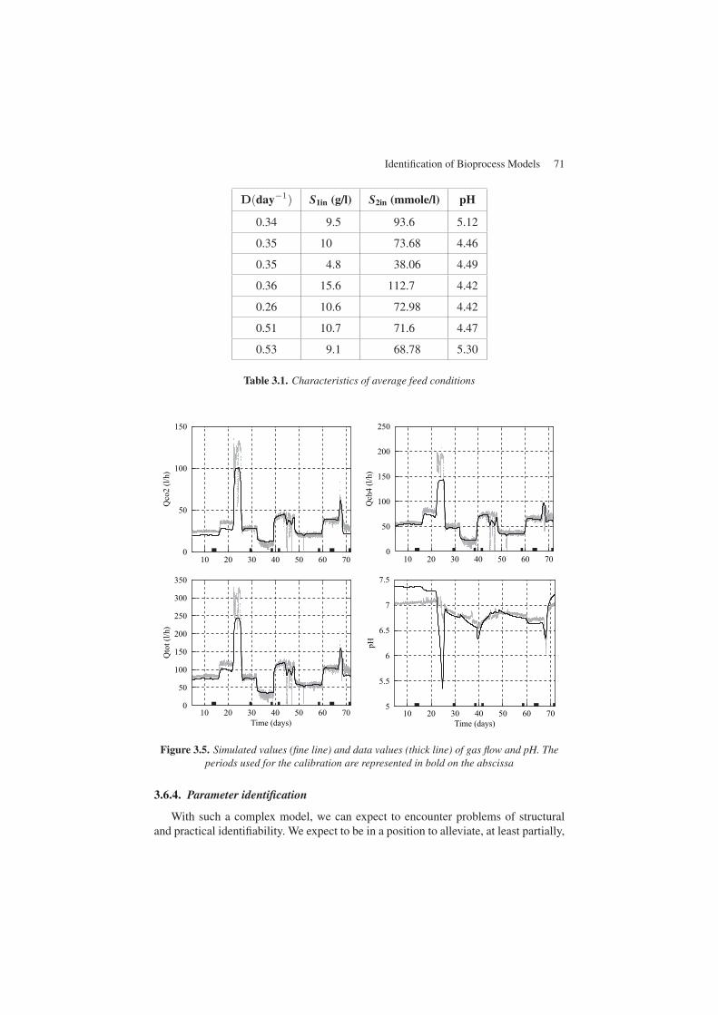
Given the complexity of the model and the large number of parameters as wellas the experimental constraints (long time constants and potential instability of theprocess), the strategy followed here for experiment design consisted of covering anumber of operating points sufficiently representative of how the process works. Theexperiment design is given in Table 3.1.
3.6.3. Choice of data for calibration and validation
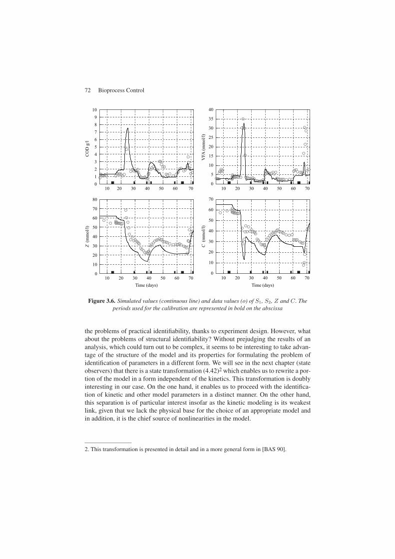
In this case, one of the priorities was to obtain a model, which would be capableof correctly reproducing as a priority the equilibrium conditions. This is why the datacollected were separated into two categories: the data corresponding to the steady-state conditions for calibrating the parameters and the dynamic data for the validation.The periods corresponding to the values used for the calibration are represented inFigures 3.5 and 3.6 by a bold line on the abscissa.
Identification of Bioprocess Models 71
D(day−1) S1in (g/l) S2in (mmole/l) pH
0.34 9.5 93.6 5.12
0.35 10 73.68 4.46
0.35 4.8 38.06 4.49
0.36 15.6 112.7 4.42
0.26 10.6 72.98 4.42
0.51 10.7 71.6 4.47
0.53 9.1 68.78 5.30
Table 3.1. Characteristics of average feed conditions
10 20 30 40 50 60 700
50
100
150
Qco
2 (l/
h)
10 20 30 40 50 60 705
5.5
6
6.5
7
7.5
pH
Time (days)10 20 30 40 50 60 70
0
50
100
150
200
250
300
350
Qto
t (l/h
)
Time (days)
10 20 30 40 50 60 700
50
100
150
200
250
Qch
4 (l/
h)
Figure 3.5. Simulated values (fine line) and data values (thick line) of gas flow and pH. Theperiods used for the calibration are represented in bold on the abscissa
3.6.4. Parameter identification
With such a complex model, we can expect to encounter problems of structuraland practical identifiability. We expect to be in a position to alleviate, at least partially,
72 Bioprocess Control
10 20 30 40 50 60 700123456789
10
CO
D g
/l
10 20 30 40 50 60 700
5
10
15
20
25
30
35
40
VFA
(mm
ol/l)
10 20 30 40 50 60 700
10
20
30
40
50
60
70C
(m
mol
/l)
Time (days)10 20 30 40 50 60 70
0
10
20
30
40
50
60
70
80
Z (m
mol
/l)
Time (days)
Figure 3.6. Simulated values (continuous line) and data values (o) of S1, S2, Z and C. Theperiods used for the calibration are represented in bold on the abscissa
the problems of practical identifiability, thanks to experiment design. However, whatabout the problems of structural identifiability? Without prejudging the results of ananalysis, which could turn out to be complex, it seems to be interesting to take advan-tage of the structure of the model and its properties for formulating the problem ofidentification of parameters in a different form. We will see in the next chapter (stateobservers) that there is a state transformation (4.42)2 which enables us to rewrite a por-tion of the model in a form independent of the kinetics. This transformation is doublyinteresting in our case. On the one hand, it enables us to proceed with the identifica-tion of kinetic and other model parameters in a distinct manner. On the other hand,this separation is of particular interest insofar as the kinetic modeling is its weakestlink, given that we lack the physical base for the choice of an appropriate model andin addition, it is the chief source of nonlinearities in the model.
2. This transformation is presented in detail and in a more general form in [BAS 90].
Identification of Bioprocess Models 73
It is basically this approach that was adopted here. As the identification is carriedout on the basis of the steady-state data, static balance equations of biomasses X1
and X2 and the expressions for the specific growth rates, we derive the followingexpressions:
1D
=α
μ1 max+KS1
α
μ1 max
1S1
(3.55)
1D
=α
μ0+KS2
α
μ0
1S2
+1KI2
α
μ0S2 (3.56)
These equations are linear in the parameters αμ1 max
, KS1α
μ1 max, α
μ0, KS2
αμ0
and1
KI2
αμ0
. They can be determined through linear regression. The only problem is that itis not possible to distinguish between μ1 max and α; this is why we have considered avalue from the literature ([GHO 74]) for μ1 max. This choice turns out to be even moreacceptable, and a sensitivity analysis shows a low sensitivity of μ1 max.
We can thus use the equation for the CO2 flow rate for determining kLa, by recall-ing that qC = kLa(CO2 −KHPC) and that the reaction for the dissociation of bicar-bonate enables the linking of CO2 to C and to pH according to the relationship:
CO2 = C1
1 +Kb10pH(3.57)
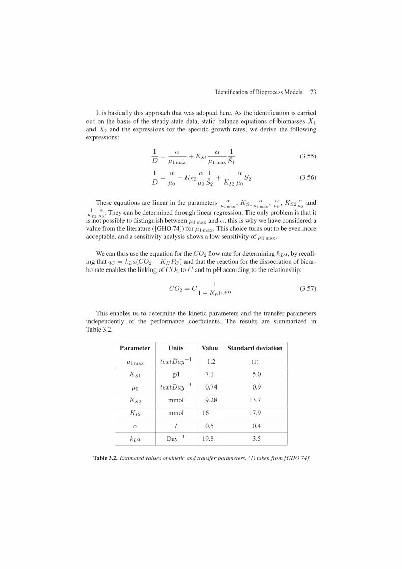
This enables us to determine the kinetic parameters and the transfer parametersindependently of the performance coefficients. The results are summarized inTable 3.2.
Parameter Units Value Standard deviation
μ1 max textDay−1 1.2 (1)
KS1 g/l 7.1 5.0
μ0 textDay−1 0.74 0.9
KS2 mmol 9.28 13.7
KI2 mmol 16 17.9
α / 0.5 0.4
kLa Day−1 19.8 3.5
Table 3.2. Estimated values of kinetic and transfer parameters. (1) taken from [GHO 74]
74 Bioprocess Control
The values of the yield coefficients now have to be calculated. The main diffi-culty results from the absence of measurements of populations X1 and X2. Withoutthese measurements, it turns out that the yield coefficients are not structurally iden-tifiable. This can be shown by considering, for example, a rescaling for X1 and X2:X ′
1 = λ1X1, X ′2 = λ2X2. This rescaling can be compensated by putting the yield
coefficients in scale as follows
k′1 =k1
λ1, k′2 =
k2
λ1, k′4 =
k4
λ1, k′3 =
k3
λ2, k′5 =
k5
λ2, k′6 =
k6
λ2(3.58)
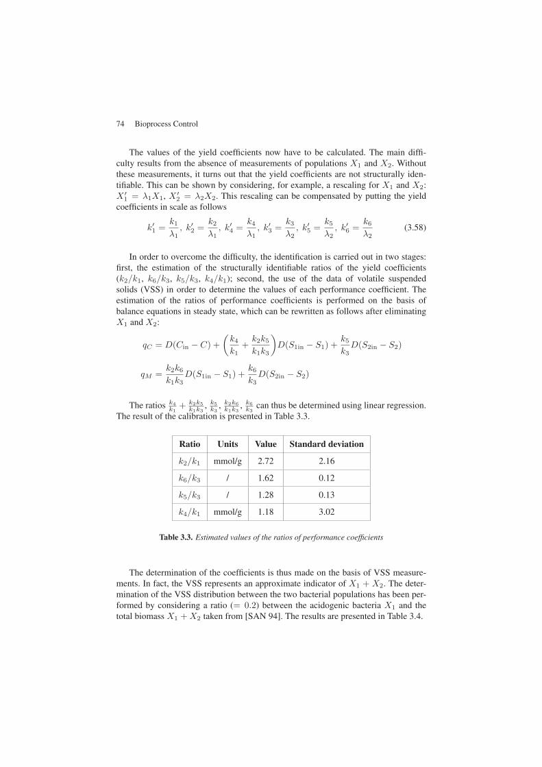
In order to overcome the difficulty, the identification is carried out in two stages:first, the estimation of the structurally identifiable ratios of the yield coefficients(k2/k1, k6/k3, k5/k3, k4/k1); second, the use of the data of volatile suspendedsolids (VSS) in order to determine the values of each performance coefficient. Theestimation of the ratios of performance coefficients is performed on the basis ofbalance equations in steady state, which can be rewritten as follows after eliminatingX1 and X2:
qC = D(Cin − C) +(k4
k1+k2k5
k1k3
)D(S1in − S1) +
k5
k3D(S2in − S2)
qM =k2k6
k1k3D(S1in − S1) +
k6
k3D(S2in − S2)
The ratios k4k1
+ k2k5k1k3
, k5k3
, k2k6k1k3
, k6k3
can thus be determined using linear regression.The result of the calibration is presented in Table 3.3.
Ratio Units Value Standard deviation
k2/k1 mmol/g 2.72 2.16
k6/k3 / 1.62 0.12
k5/k3 / 1.28 0.13
k4/k1 mmol/g 1.18 3.02
Table 3.3. Estimated values of the ratios of performance coefficients
The determination of the coefficients is thus made on the basis of VSS measure-ments. In fact, the VSS represents an approximate indicator of X1 + X2. The deter-mination of the VSS distribution between the two bacterial populations has been per-formed by considering a ratio (= 0.2) between the acidogenic bacteria X1 and thetotal biomass X1 +X2 taken from [SAN 94]. The results are presented in Table 3.4.
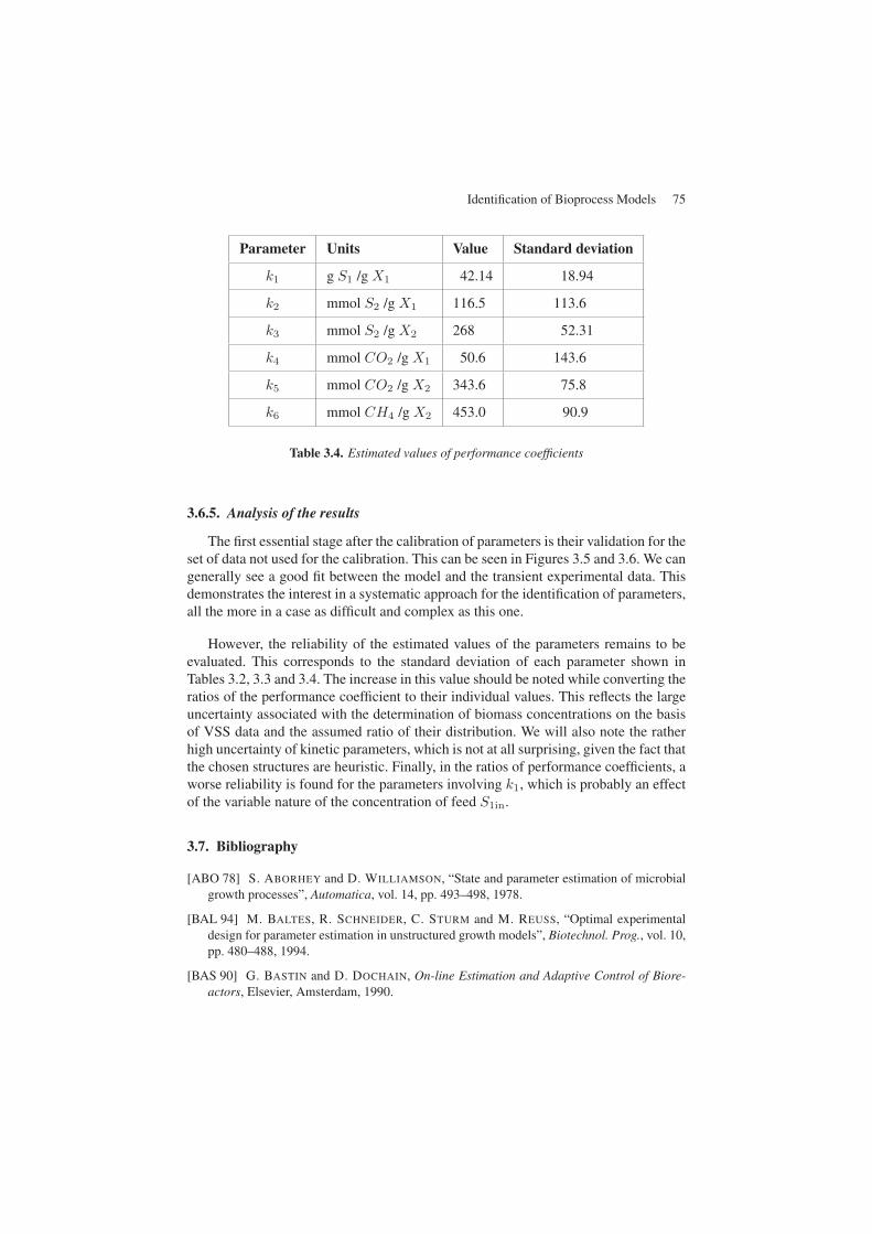
Identification of Bioprocess Models 75
Parameter Units Value Standard deviation
k1 g S1 /g X1 42.14 18.94
k2 mmol S2 /g X1 116.5 113.6
k3 mmol S2 /g X2 268 52.31
k4 mmol CO2 /g X1 50.6 143.6
k5 mmol CO2 /g X2 343.6 75.8
k6 mmol CH4 /g X2 453.0 90.9
Table 3.4. Estimated values of performance coefficients
3.6.5. Analysis of the results
The first essential stage after the calibration of parameters is their validation for theset of data not used for the calibration. This can be seen in Figures 3.5 and 3.6. We cangenerally see a good fit between the model and the transient experimental data. Thisdemonstrates the interest in a systematic approach for the identification of parameters,all the more in a case as difficult and complex as this one.
However, the reliability of the estimated values of the parameters remains to beevaluated. This corresponds to the standard deviation of each parameter shown inTables 3.2, 3.3 and 3.4. The increase in this value should be noted while converting theratios of the performance coefficient to their individual values. This reflects the largeuncertainty associated with the determination of biomass concentrations on the basisof VSS data and the assumed ratio of their distribution. We will also note the ratherhigh uncertainty of kinetic parameters, which is not at all surprising, given the fact thatthe chosen structures are heuristic. Finally, in the ratios of performance coefficients, aworse reliability is found for the parameters involving k1, which is probably an effectof the variable nature of the concentration of feed S1in.
3.7. Bibliography
[ABO 78] S. ABORHEY and D. WILLIAMSON, “State and parameter estimation of microbialgrowth processes”, Automatica, vol. 14, pp. 493–498, 1978.
[BAL 94] M. BALTES, R. SCHNEIDER, C. STURM and M. REUSS, “Optimal experimentaldesign for parameter estimation in unstructured growth models”, Biotechnol. Prog., vol. 10,pp. 480–488, 1994.
[BAS 90] G. BASTIN and D. DOCHAIN, On-line Estimation and Adaptive Control of Biore-actors, Elsevier, Amsterdam, 1990.
Chapter 7
Adaptive Linearizing Control andExtremum-Seeking Control
of Bioprocesses
7.1. Introduction
Industrial-scale biotechnological processes have progressed vigorously over recentdecades. As already mentioned, the problems arising from the implementation of theseprocesses are similar to those of more classical industrial processes and the need forautomatic control in order to optimize production efficiency, improve product qualityor detect disturbances in process operation is obvious. Nevertheless, automatic controlof industrial biotechnological processes is facing two major difficulties:
a) it remains difficult to develop models taking into account the numerous factorsthat can influence microorganism growth and other biochemical reactions;
b) another essential difficulty lies in the absence, in most cases, of cheap and reli-able instrumentation suited to real-time monitoring.
The classical monitoring and control methods do not prove very efficient to tideover these difficulties. The efficiency of any control system highly depends on thedesign of the control and monitoring techniques and the care taken in their design. Infact, monitoring or control algorithms will prove to be efficient if they are able to incor-porate the important well-known information on the process while being able to dealwith the missing information (lack of online measurements, uncertainty on the dynam-ics, etc.) in a “robust” way, i.e. such that the missing information will not significantly
Chapter written by Denis DOCHAIN, Martin GUAY, Michel PERRIER and Mariana TITICA.
173
174 Bioprocess Control
deteriorate the control performance of the process. The versatility of computing plat-forms greatly facilitates the design and implementation of sophisticated controllers(beyond the classical PID as presented in Chapter 6). These controllers may arise fromquite complex theory (nonlinear control, adaptive control, extremum-seeking control)but, as will be shown, their structure and implementation will remain rather simplewhile including the key features of simple PIDs.
In this chapter, we shall show how to incorporate the well-known features of thedynamics of biochemical processes (basically, the reaction network and the materialbalances) in control algorithms which are capable of dealing with process uncertainty(in particular on the reaction kinetics) by introducing, an adaptation scheme for exam-ple in the control algorithms.
It is also important to draw to the attention of the reader that these control systemsare not just the object of academic research but are already used in several applications(see e.g. [BAS 90, CHE 91]). Adaptive as well as non-adaptive linearizing control ofbioreactors has been a quite active research area over recent decades. In addition tothe works by the authors of this chapter and their colleagues, let us also mention e.g.[ALV 88, CHI 91, DAH 91, FLA 91, GOL 86, HEN 92, HOO 86].
The chapter is organized as follows. We shall first concentrate on the design ofadaptive linearizing controllers for bioprocesses based on a reduced order model ofthe process. The methodology will be illustrated by anaerobic digestion and activatedsludge. We shall then consider online optimization approaches, adaptive extremum-seeking control, whose specificity is to combine feedback control with a search algo-rithm for the optimal process operating conditions. In that section, we shall considerthe illustrative example of fed-batch reactors.
7.2. Adaptive linearizing control of bioprocesses
7.2.1. Design of the adaptive linearizing controller
Let us first concentrate on the design of model-based controllers for bioreactors.The key idea of the control design is here again to take advantage of what is wellknown about the dynamics of bioprocesses (reaction network and mass balances)which are summarized in the general dynamic model already presented in the pre-ceding chapters:
dξ
dt= Kr(ξ) + F −Q−Dξ (7.1)
while taking into account the model uncertainty (mainly the kinetics). Since the modelis generally nonlinear, the model-based control design will result in a linearizing con-trol structure, in which the online estimation of the unknown variables (component
188 Bioprocess Control
The auxiliary variables ζ, the unknown parameters and tuning estimation variableshave been initialized as follows:
ζ1 = 1400 mg/l, ζ2 = 750 mg/l, ζ3 = 1400 mg/l, g1,0 = g2,0 = 10−3
γ1 = γ2 = 0.9, α1,0 = α2,0 = 0.00025 l2/mg2/h
Note the ability of the controller to maintain the controlled outputs S and C closeto their desired values in spite of the unknown disturbance.
7.3. Adaptive extremum-seeking control of bioprocesses
Most adaptive control schemes documented in the literature (e.g. [AST 95,GOO 84, KRS 95, NAR 89]) are developed for regulation to known set-points ortracking known reference trajectories. In some applications, however, the controlobjective could be to optimize an objective function which can be a functionof unknown parameters, or to select the desired values of the state variables tokeep a performance function at its extremum value. Self-optimizing control andextremum-seeking control are two methods of handling these types of optimizationproblems. The task of extremum seeking is to find the operating set-points thatmaximize or minimize an objective function. Since the early research work onextremum control in the 1920s [LEB 22], several applications of extremum controlapproaches have been reported (e.g. [AST 95, DRK 95, STE 80, VAS 57]). Krstic etal. [KRS 00a, KRS 00b] presented several extremum control schemes and stabilityanalysis for extremum-seeking of linear unknown systems and a class of generalnonlinear systems [KRS 00a, KRS 00b, KRS 98]. A neural network-based approachhas been proposed in [LI 95].
The implications for the biochemical industry are clear. In this sector, it is rec-ognized that even small performance improvements in key process control variablesmay result in substantial economic gains. As an example, the potential benefits ofextremum-seeking techniques in the maximization of biomass production rate in well-mixed biological processes has been demonstrated in [WAN 99].
The proposed scheme utilizes explicit structure information of the objective func-tion that depends on system states and unknown plant parameters. This scheme isbased on Lyapunov’s stability theorem. As a result, global stability is ensured duringthe seeking of the extremum of the nonlinear stirred tank bioreactors. It is also shownthat once a certain level of persistence of excitation (PE) condition is satisfied, theconvergence of the extremum-seeking mechanism can be guaranteed. In this sectionwe concentrate on the adaptive extremum-seeking control of bioreactors operating inthe fed-batch mode (see also [TIT 03a, TIT 03b]) but several other alternatives of thesimilar schemes (including the use of universal approximation like artificial neuralnetworks (ANN)) have been proposed in the literature for different bioprocess config-urations [GUA 04, HAR 06, MAR 04, MAR 03, ZHA 02].
Adaptive Linearizing Control and Extremum-Seeking Control of Bioprocesses 189
7.3.1. Fed-batch reactor model
Fed-batch bioreactors represent an important class of bioprocesses, mainly in thefood industry and in the pharmaceutical industry but also e.g. for biopolymer applica-tions (PHB). One of the key issues in the operation of fed-batch reactors is to optimizethe production of a synthesis product (e.g. penicillin, enzymes, etc.) or biomass (e.g.baker’s yeast). They are therefore ideal candidates for optimal control strategies. Aintensive research activity was devoted to optimal control of (fed-batch) bioreactorsmainly in the 1970s and in the 1980s (see e.g. [OHN 76, CHE 79, PAR 85, PER 79]).However, in practice, because of the large uncertainty related to the modeling of theprocess dynamics [BAS 90], poor performance may be expected from such controlstrategies, and although a priori attractive, optimal control has not been largely appliedto industrial bioprocesses. Alternative approaches have been proposed for handlingthe process uncertainties with an adaptive control scheme (e.g. [DOC 89, VAN 93]).In this approach, we propose to go a step further by including a static optimum searchin the adaptive control scheme.
Consider the following dynamic model of a simple microbial growth process withone gaseous product in a fed-batch reactor:
dX
dt= μX −DX (7.52)
dS
dt= −k1μX +D(S0 − S) (7.53)
y = k2μX (7.54)
dv
dt= Dv (7.55)
where statesX (g/l) and S (g/l) hold for biomass and substrate concentrations, respec-tively. μ (h−1) is the specific growth rate, D (h−1) is the dilution rate, y (g/l/h) is theproduction rate of the reaction product, S0 (g/l) denotes the concentration of the sub-strate in the feed, k1, k2 are yield coefficients, and v (l) is the volume of liquid mediumin the tank. A typical situation in bioprocess applications is when the biomass concen-tration is not available for online measurement while the gaseous outflow rate y (e.g.CO2) is easier to measure online. We consider here that only S and y are measurablewhile the biomass concentration X is not available for feedback control.
In this work, we consider the extremum-seeking problem for the bioprocess model(7.52)-(7.55) with a specific growth rate μ expressed by the Haldane model. Thismodel (see Figure 7.3) is given by:
μ =μ0S
KS + S + S2
KI
(7.56)
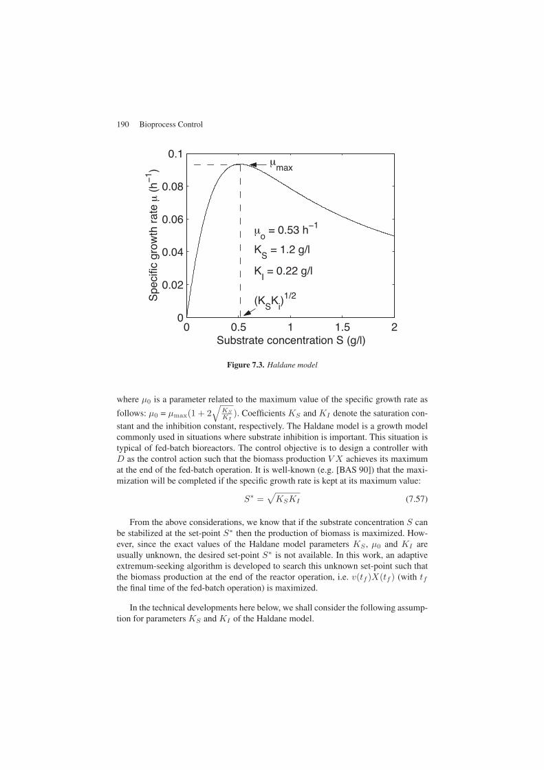
190 Bioprocess Control
Figure 7.3. Haldane model
where μ0 is a parameter related to the maximum value of the specific growth rate as
follows: μ0 = μmax(1 + 2√
KS
KI). Coefficients KS and KI denote the saturation con-
stant and the inhibition constant, respectively. The Haldane model is a growth modelcommonly used in situations where substrate inhibition is important. This situation istypical of fed-batch bioreactors. The control objective is to design a controller withD as the control action such that the biomass production V X achieves its maximumat the end of the fed-batch operation. It is well-known (e.g. [BAS 90]) that the maxi-mization will be completed if the specific growth rate is kept at its maximum value:
S∗ =√KSKI (7.57)
From the above considerations, we know that if the substrate concentration S canbe stabilized at the set-point S∗ then the production of biomass is maximized. How-ever, since the exact values of the Haldane model parameters KS , μ0 and KI areusually unknown, the desired set-point S∗ is not available. In this work, an adaptiveextremum-seeking algorithm is developed to search this unknown set-point such thatthe biomass production at the end of the reactor operation, i.e. v(tf )X(tf ) (with tfthe final time of the fed-batch operation) is maximized.
In the technical developments here below, we shall consider the following assump-tion for parameters KS and KI of the Haldane model.
Adaptive Linearizing Control and Extremum-Seeking Control of Bioprocesses 191
Assumption: KS and KI are known to be bounded as follows: KS,min ≤ KS ≤KS,max, 0 < KI ≤ KI,max.
This assumption is only important for the technical developments in order to avoidsingularities in the extremum-seeking controller. It should not be interpreted as a“microbial” constraint on the kinetic model.
7.3.2. Estimation and controller design
The design of the adaptive extremum-seeking controller will proceed in differentsteps. First of all, we shall start with the estimation equation for y, then include thecontroller equations and the estimation equations for the unknown parameters in aLyapunov-based derivation framework, and end up with the stability and convergenceanalysis arguments.
7.3.2.1. Estimation equation for the gaseous outflow rate y
Let us start with the parameter estimation algorithm for the unknown parametersKS , KI and μ0. The ratio of the yield coefficients k1
k2is assumed to be known. It
follows from (7.54) that:
μX =y
k2(7.58)
Then equations (7.52)-(7.53) can be reformulated as follows:
dX
dt=
1k2y −DX (7.59)
dS
dt= −k1
k2y +D(S0 − S) (7.60)
By considering equations (7.54)-(7.56) and (7.59)-(7.60), the time derivative of yis equal to:
dy
dt= k2μ0X
KS − S2/KI(KS + S + S2/KI
)2(− k1
k2y +D(S0 − S)
)
+ k2μ
[1k2y −DX
] (7.61)
Since the biomass concentration X is not accessible for online measurement, wereformulate dy
dt by replacing X with yk2μ as follows:
dy
dt=
Ks − S2
KI
S(KS + S + S2
KI
)(− k1
k2y2 +D
(S0 − S
)y
)+ μy −Dy (7.62)
192 Bioprocess Control
Let θ = [θs θμ θi]T with θμ = μ0KS
, θs = 1KS
, θi = 1KIKS
, and define θk = k1k2
.Equations (7.60) and (7.62) can then be rewritten as follows:
dS
dt= −θky +D
(S0 − S
)(7.63)
dy
dt=
1− θiS2
S(1 + θsS + θiS2)(D(S0 − S
)− θky)y
+θμSy
1 + θsS + θiS2− uy
(7.64)
Let θ denote the estimate of the true parameter θ, and y be the prediction of y byusing the estimated parameter θ. The predicted state y is generated by the followingequation:
dy
dt=
1− θiS2
S(1 + θsS + θiS2
)(D(S0 − S)− θky
)y
+θμSy
1 + θsS + θiS2−Dy + kyey
(7.65)
with ky > 0 and the prediction error ey = y − y. It follows from (7.63)-(7.65) that:
dey
dt= −kyey +
1− θiS2
s(1 + θsS + θiS2
)(D(S0 − S)− θky
)y
+θμSy
1 + θsS + θiS2− 1− θiS
2
S(1 + θsS + θiS2
)(D(S0 − S)− θky
)y
− θμSy
1 + θsS + θiS2
(7.66)
7.3.2.2. Design of the adaptive extremum-seeking controller
The desired set-point (7.57) can be re-expressed as follows:
S∗ =1√θi
(7.67)
Since parameter θi is unknown, we design a controller to drive the substrate con-centration S to:
1√θi
i.e. an estimate of the unknown optimum S∗. An excitation signal is then designedand injected into the adaptive system such that the estimated parameter θi convergesto its true value. The extremum-seeking control objective can be achieved when thesubstrate concentration S is stabilized at the optimal operating point S∗.
Adaptive Linearizing Control and Extremum-Seeking Control of Bioprocesses 193
Define the “control” error zs:
zs = S − 1√θi
− d(t) (7.68)
where d(t) ∈ C1 is a dither signal that will be assigned later. The time derivative ofzs is given by:
dzs
dt= D
(S0 − S
)− θky +12θ− 3
2i
dθi
dt− d(t) = Γ1 (7.69)
We consider a Lyapunov function candidate:
V =z2
s
2+
12
(θ2μγμ
+θ2sγs
+θ2iγi
)+(1 + θsS + θiS
2)e2y
2(7.70)
with constants γμ, γs, γi > 0. Taking the time derivative of V and substituting (7.63),(7.69) and (7.66) leads to:
dV
dt= zsΓ1 − θμ
γμ
dθμ
dt− θs
γs
dθs
dt− θi
γi
dθi
dt
+ ey
(1− θiS
2)
S
(D(S0 − S
)− θky)y + eyθμSy
− ey
(1− θiS
2
S(1 + θsS + θiS2
)(D(S0 − S)− θky
)y
+θμSy
1 + θsS + θiS2
)(1 + θsS + θiS
2)
− e2y[(
ky −(θs + 2θiS
)(S0 − S
)D
2(1 + θsS + θiS2) )(
1 + θsS + θiS2)
+12(θs + 2θiS
)θky
]
(7.71)
Defining the functions:
Γ = −e2y(ky −
(θs + 2θiS
)(S0 − S
)D
2(1 + θsS + θiS2
) )(1 + θsS + θiS
2)
− 12e2y(θs + 2θiS
)θky
(7.72)
Ψi = Γ3D + Γ4 (7.73)
Ψμ = eySy (7.74)
Ψs = Γ5D + Γ6 (7.75)
194 Bioprocess Control
where:
Γ3 = −eyS(S0 − S
)y − eyS
(1− θiS
2)(S0 − S
)y
1 + θsS + θiS2(7.76)
Γ4 = eySθky2 +
eyS(1− θiS
2)θky
2
1 + θsS + θiS2− eyS
3θμy
1 + θsS + θiS2(7.77)
Γ5 = −ey
(1− θiS
2)(S0 − S
)y
1 + θsS + θiS2(7.78)
Γ6 =ey
(1− θiS
2)θky
2
1 + θsS + θiS2− ey θμS
2y
1 + θsS + θiS2(7.79)
we can write dVdt as follows:
dV
dt= zs
[D(S0 − S
)− θky +12θ− 3
2i
dθi
dt− d(t)
]+(
Ψi − 1γi
dθi
dt
)θi
+(
Ψμ − 1γμ
dθμ
dt
)θμ +
(Ψs − 1
γs
dθs
dt
)θs + Γ
(7.80)
For the solution of the extremum-seeking problem, we pose the dynamic statefeedback:
d(t) = a(t) +12θ− 3
2i
dθi
dt− kdd(t) (7.81)
D =1
S0 − S[− kzzs + θky + a(t)− kdd(t)
], kz > 0 (7.82)
where a(t) acts as a dither signal on the closed-loop process and kd is a strictly positiveconstant.
The substitution of (7.82) in (7.80) yields:
dV
dt= −kzz
2s +(
Ψi −˙θi
γi
)θi +
(Ψμ −
˙θμ
γμ
)θμ +
(Ψs −
˙θs
γs
)θsΓ + Γ (7.83)
Using the definition of Ψi and Ψs, we express (7.83) as:
dV
dt= −kzz
2s +(
Γ3D + Γ4 −˙θi
γi
)θi +
(Ψμ −
˙θμ
γμ
)θμ
+(
Γ5D + Γ6 −˙θs
γs
)θsΓ
(7.84)
Adaptive Linearizing Control and Extremum-Seeking Control of Bioprocesses 195
We propose the following update law as follows:
˙θi =
{γi
(Γ3D + Γ4
), if θi > εi or θi = εi and
(Γ3D + Γ4
)> 0
0 otherwise(7.85)
˙θs =
{γs
(Γ5D + Γ6
), if θs > εs or θs = εs and
(Γ5D + Γ6
)> 0
0 otherwise(7.86)
˙θμ = γμΨμ (7.87)
with the initial condition θs(0)≥ εs = 1KS,max
>0, and θi(0)≥ εi = 1Ks,maxKI,max
>0.
The update laws (7.85)-(7.86) are projection algorithms that ensure that θs(t)≥εs>0and θi(t) ≥ εi > 0. They also ensure that:(
Γ3D + Γ4 −˙θi
γi
)θi +
(Ψμ −
˙θμ
γμ
)θμ +
(Γ5D + Γ6 −
˙θs
γs
)θs ≤ 0, (7.88)
7.3.2.3. Stability and convergence analysis
Substituting the update laws (7.85)-(7.86) into (7.84), we obtain:
dV
dt≤ −kzz
2s + Γ (7.89)
We then assign the gain function ky such that the term Γ is negative. Using (7.72),we consider:
ky = ky0 +
(S0 − S
)|D|ε(S + ε)
(7.90)
with positive constants ky0 > 0 and 0 < ε� 1. As a result, we obtain:
dV
dt≤ −kzz
2s − ky0
(1 + θsS + θiS
2)e2y (7.91)
as required. Following LaSalle-Yoshizawa’s Theorem, it is concluded that θ, zs andey are bounded, and:
limt→∞ zs = 0, lim
t→∞ ey = 0 (7.92)
This implies that:
limt→∞
˙θi(t) = 0, lim
t→∞˙θμ(t) = 0, lim
t→∞˙θs(t) = 0.
196 Bioprocess Control
Hence, the auxiliary variable d(t) is bounded if a(t) is bounded and d(t) tendstowards zero if a(t) does. Thus, all signals of the closed-loop system are bounded.It should be noted that the convergence of the state error ey does not mean that theestimated parameters converge to their true values as t → ∞. In section 7.4, weinvestigate the condition that guarantees the parameter convergence.
7.3.2.4. A note on dither signal design
The results of the previous section confirm the convergence of the extremum-seeking scheme if the persistency of excitation (PE) condition (7.116) is encountered.It remains fairly difficult to ensure that the dither signal employed is sufficiently rich.One of the main difficulties is that the calculation of the PE condition criteria dependson the value of the unknown parameters. In this study, we use the asymptotic value ofthe PE condition (7.116) to test whether a given dither signal is sufficiently exciting.The approach can be summarized as follows.
As t→∞, the analysis detailed above confirms that limt→∞ zs = 0. This meansthat asymptotically, the substrate concentration S converges to 1√
θi
+ d(t). Since θi
converges to a constant value, the asymptotic dynamics of the substrate concentration,S∞, coincide with the dynamics of the dither signal given (7.81) which converge to
dS∞dt
= d = a(t)− kdd(t) (7.93)
as t→∞. The asymptotic dynamics of the production rate y∞ are given by:
dy∞dt
=
(1− θiS∞
S∞(1 + θsS∞ + θiS∞2
)(a(t)− kdd(t))
+θμS∞(
1 + θsS∞ + θiS∞2) +
1(S0 − S∞
)(a(t)− kdd(t)))y∞
− θk
S0 − S∞y∞2.
(7.94)
If we assume that a set of possible values of parameters θi, θμ and θs can beobtained, (7.93)-(7.94) can be solved for a given set of initial conditions and externalsignal a(t). The corresponding trajectories are estimates of the asymptotic trajectoriesof the system subject to the extremum-seeking control. For each specific trajectory,we can calculate the corresponding value of the matrix:∫ t+T0
t
Ψ∞(τ)dτ. (7.95)
Adaptive Linearizing Control and Extremum-Seeking Control of Bioprocesses 197
where Ψ∞(t)=Φa(S∞, y∞, u∞, θ)Φa(S∞, y∞, u∞, θ)T with u∞= 1(S0−S∞) (θky∞
+ a(t)− kdd(t)):
Φa
(S∞, y∞, θ, u∞
)=
⎡⎢⎣−2γuS∞2 − γuS∞3θs − S∞4y∞θμ
−γuS∞ + γuS∞3θi − θμS∞3y∞S∞2y∞ + θsS∞3y∞ + θiS∞4y∞
⎤⎥⎦ (7.96)
and γu = (a(t)− kdd(t))y∞.
The strategy for testing any specific dither signal consists of evaluating the mini-mum eigenvalue of matrix (7.95) over a specific time horizon. If the minimum eigen-value is positive for all t > 0, the dither signal is deemed sufficiently rich and its usecan be justified on the closed-loop extremum-seeking control system.
It is important to note that the corresponding conclusion depends entirely on thespecific choice of parameter values that are used in the calculations. More work isrequired to investigate how this assessment can be conducted in a manner that is invari-ant of the choice of parameter values.
The use of this technique will be considered in the simulation study presented inthe next section.
7.3.3. Simulation results
The aim of this section is to illustrate the performance of an adaptive extremum-seeking controller in a number of simulations, performed using a realistic example ofa fed-batch process. The kinetic model parameters, yield coefficients and initial statesused during numerical simulations are:
μ0 = 0.53 h−1, KS = 1.2 g/l, KI = 0.22 g/l, k1 = 0.4, k2 = 1
X(0) = 7.2 g/l, S(0) = 2 g/l, S0 = 20 g/l(7.97)
For the Haldane model, from Figure 7.3, the maximum on the growth specificrate occurs at S∗ = 1√
θi= 0.52 g/l. The control objective is to design a controller
for the dilution rate, u, to regulate substrate S at S∗. The controller requires onlinemeasurements of variables S and y, as well as the knowledge of the kinetic param-eters, determining the S∗. These values are obtained using the estimation algorithmpreviously presented, using the measurements of y.
For the simulation study, we consider the following initial estimates of the kineticparameters:
θμ = 1, θS = 0.1, θI = 3(μ0 = 10, KS = 10, KI = 0.03
)(7.98)
198 Bioprocess Control
The design parameters for the extremum-seeking controller are set to:
γμ = 10, γS = 200, γi = 200 ky,0 = 20, kz = 0.5, kd,0 = 1, ε = 0.2
Dither signal a(t) is chosen as follows:
a(t) =5∑
i=1
A1isin((
0.001 + (5− 0.001)i/4)t)
+5∑
i=1
A2icos((
0.01 + (5− 0.01)i/4)t) (7.99)
where A1i and A2i are normally distributed random numbers in the interval[−0.1, 0.1].
To test the richness of the dither signal, we calculate the smallest eigenvalueof matrix (7.95) over the interval [0, 100] using the initial conditions, x(0) = 7.2,s(0) = 1/
√3 and parameter estimates given by (7.98).
The simulation shows that the signal is sufficiently exciting in a region of theseinitial conditions and parameter values. The resulting dither signal was used in thesubsequent simulation of the extremum-seeking control scheme. It should be notedthat it is relatively easy in practice to provide a dither signal such that matrix (7.95) ispositive definite. However, the convergence of the parameter estimates can also dependon the conditioning of this matrix. The calculations demonstrate that the conditionnumber of the matrix remains around 103, a value that is relatively high. This indicatesthat parameter convergence may remain quite slow. In fact, a closer look at the spectraldecomposition of this matrix indicates that the poor conditioning is associated with theadaptation of θs.
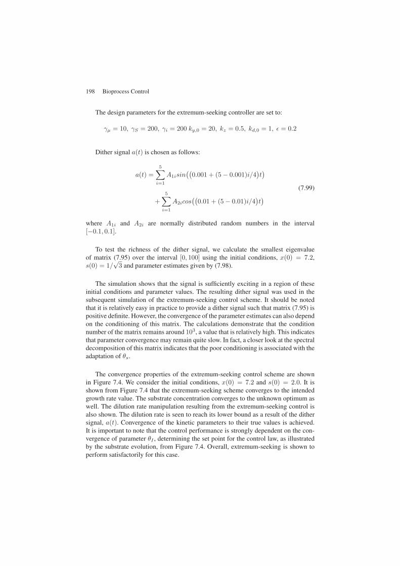
The convergence properties of the extremum-seeking control scheme are shownin Figure 7.4. We consider the initial conditions, x(0) = 7.2 and s(0) = 2.0. It isshown from Figure 7.4 that the extremum-seeking scheme converges to the intendedgrowth rate value. The substrate concentration converges to the unknown optimum aswell. The dilution rate manipulation resulting from the extremum-seeking control isalso shown. The dilution rate is seen to reach its lower bound as a result of the dithersignal, a(t). Convergence of the kinetic parameters to their true values is achieved.It is important to note that the control performance is strongly dependent on the con-vergence of parameter θI , determining the set point for the control law, as illustratedby the substrate evolution, from Figure 7.4. Overall, extremum-seeking is shown toperform satisfactorily for this case.
Adaptive Linearizing Control and Extremum-Seeking Control of Bioprocesses 199
0.1
0.09
0.08
0.07
0.06
0.05
0.04
0.03
μ(S
)gl−
1hr
−1
μ(S)μ(S)∗
0 10 20 30 40 50 60 70 80 90 100
Time (hr)
0.12
0.1
0.08
0.06
0.04
0.02
0
Dilu
tion
Rat
ehr
−1
0 10 20 30 40 50 60 70 80 90 100
Time (hr)
3
2.5
2
1.5
1
0.5
0
Sgl
−1
SS∗
0 10 20 30 40 50 60 70 80 90 100
Time (hr)
6
5
4
3
2
1
0
−1
−2
θs,θ
i,θ
μ
0 10 20 30 40 50 60 70 80 90 100
Estimated θTrue θ
Time (hr)
Figure 7.4. Illustration of the convergence properties
In Krstic et al., an extremum-seeking scheme was proposed to optimize the pro-duction rate for a class of bioreactors governed by Monod kinetics and Haldane kinet-ics [WAN 99]. An extremum-seeking control was developed following the design pro-cedure proposed in [WAN 99]. The main difference is that we use the procedure tooptimize the growth rate μ(S). In this case, the extremum-seeking scheme yields theclosed-loop system:
x = (μ−D)x
S = −k1μx+ (S0 − S)D
˙D = k(μ− η) + a sin(ωt)
η = ωh(μ− η)D = D + a sin(ωt)
(7.100)
where μ is given by (7.56). Note that the structure assumes that the actual value of μis measured in this case. This is extremely unlikely since this would require detailedstructural information about the parameter values of μmax, Ks and Ki entering theexpression for μ.
200 Bioprocess Control
0.1
0.09
0.08
0.07
0.06
0.05
0.04
0.03
0.02
μ(S
)gl−
1hr
−1
μ(S)μ(S)∗
0 20 40 60 80 100 120 140 160 180 200
Time (hr)
0.1
0.09
0.08
0.07
0.06
0.05
0.04
0.03
μ(S
)gl−
1hr
−1
μ(S)μ(S)∗
0 20 40 60 80 100 120 140 160 180 200
Time (hr)
0.06
0.05
0.04
0.03
0.02
0.01
0
Dilu
tion
Rat
ehr
−1
0 20 40 60 80 100 120 140 160 180 200
Time (hr)
0.2
0.18
0.16
0.14
0.12
0.10
0.08
0.06
0.04
0.02
0
Dilu
tion
Rat
ehr
−1
0 20 40 60 80 100 120 140 160 180 200
Time (hr)
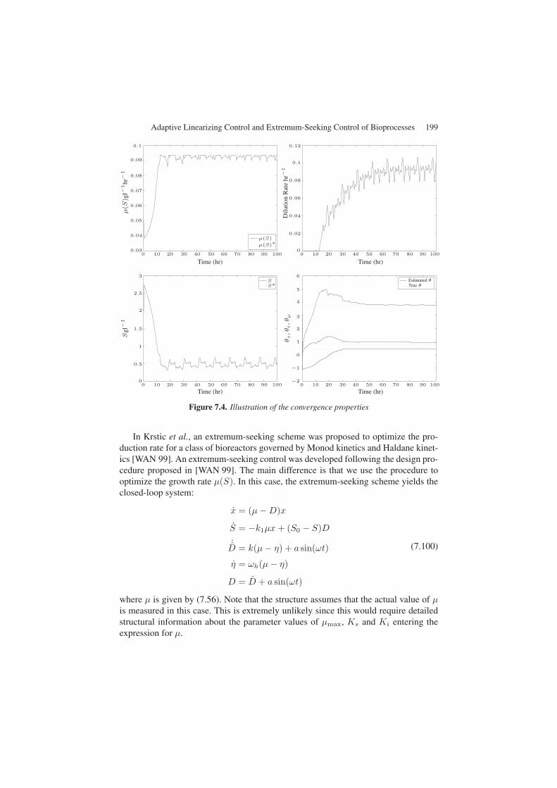
Figure 7.5. Performance of the proposed scheme (right) and the controller proposed in[WAN 99] for the case x(0) = 7.2, s(0) = 2.0
In order to facilitate the comparison, the tuning parameters of the extremum-seeking scheme are set to the following values:
a = 0.01, ω = 0.75, k = 5, ωh = 0.1
The tuning parameters were assigned following the guidelines outlined in[KRS 00a]. Two simulations were performed. The first simulation was initiated atX(0) = 7.2, S(0) = 2.0, as above. Figure 7.5 shows the comparison between theperformance of the two extremum-seeking schemes. On the left hand side, we showthe dilution rate and specific growth rate μ for the proposed extremum-seeking con-troller. On the right side, we show the dilution rate and specific growth rate resultingfrom the application of the extremum-seeking scheme proposed in [WAN 99]. Theresults demonstrate that the two control schemes provide comparatively equivalentconvergence properties. The scheme of [WAN 99] provides a slower convergencewhich could be improved by further adjustments of the design parameters. The valuesemployed were the values that were found to provide the best performance for thissystem.
Adaptive Linearizing Control and Extremum-Seeking Control of Bioprocesses 201
0.1
0.09
0.08
0.07
0.06
0.05
0.04
0.03
0.02
0.01
0
μ(S
)gl−
1hr
−1
μ(S)μ(S)∗
0 50 100 150 200 250 300 350 400 450 500
Time (hr)
0.095
0.09
0.085
0.08
0.075
0.07
0.065
0.06
0.055
0.05
0.045
μ(S
)gl−
1hr
−1
μ(S)μ(S)∗
0 50 100 150 200 250 300 350 400 450 500
Time (hr)
0.06
0.05
0.04
0.03
0.02
0.01
0
Dilu
tion
Rat
ehr
−1
0 50 100 150 200 250 300 350 400 450 500
Time (hr)
0.12
0.1
0.08
0.06
0.04
0.02
0
μ(S
)gl−
1hr
−1
0 50 100 150 200 250 300 350 400 450 500
Time (hr)
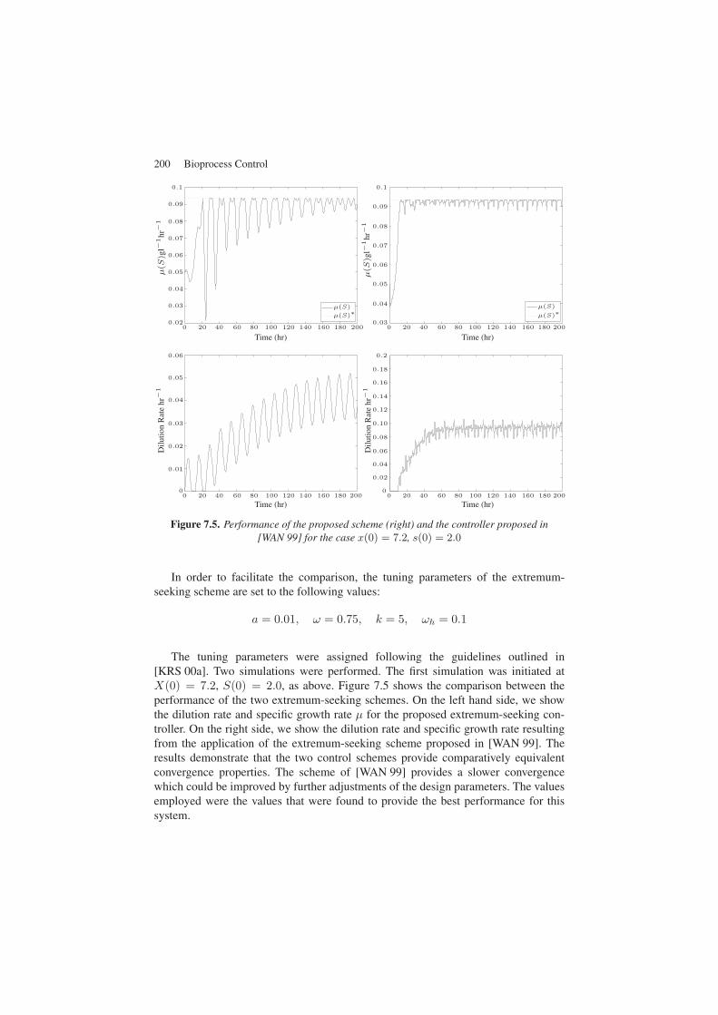
Figure 7.6. Performance of the proposed scheme (right) and the controller proposed in[WAN 99] for the case x(0) = 1.2, s(0) = 2.0
In the second simulation, the initial concentration of biomass was set to X(0) =1.2. The simulation results are shown in Figure 7.6. As above, we show the dilutionrate and specific growth rate for the proposed scheme on the right hand side and theresults for the controller proposed by [WAN 99] on the left hand side. The schemeproposed in [WAN 99] provides very poor convergence properties compared to thescheme proposed here.
Overall, the results indicate that the proposed scheme provides very consistentperformance for this system.
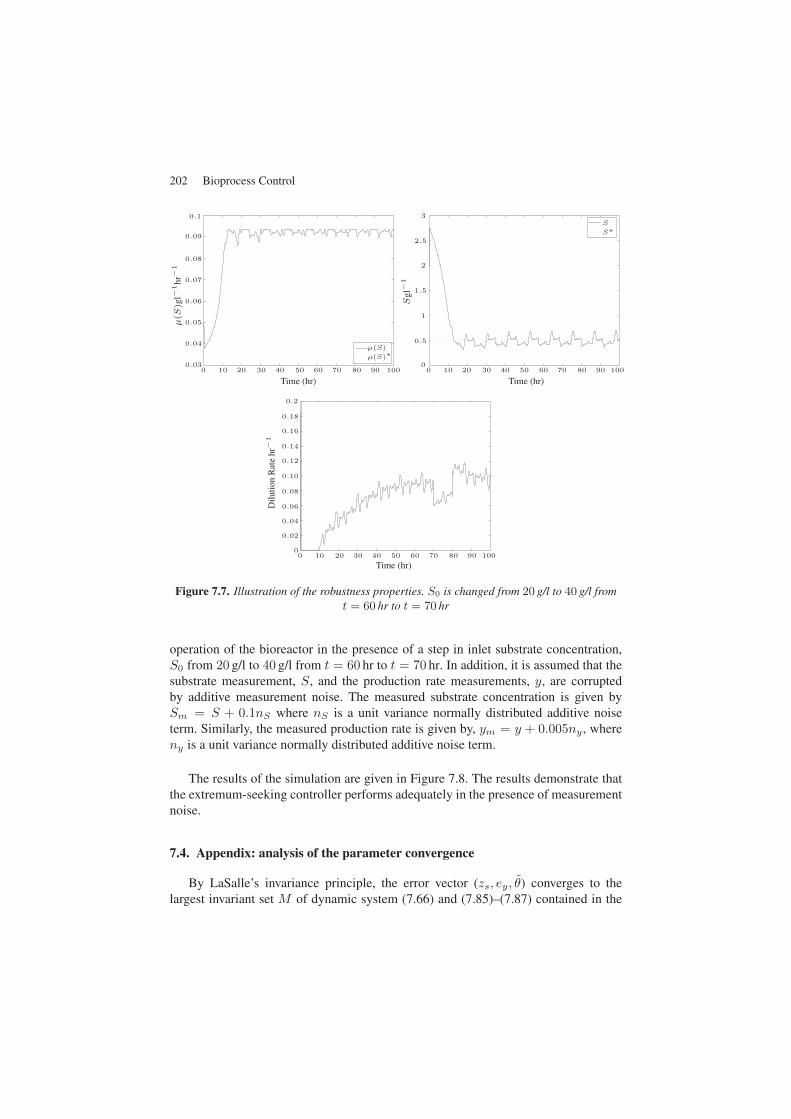
In the next set of simulations, we wish to illustrate the controller performancefor regulation (as illustrated in Figure 7.7) by introducing a disturbance in the S0
concentration between 60 and 70 hours. As expected, the controller quickly rejectsthe disturbance while attenuating its effect on S which is accurately regulated at theset point during the whole operation.
The last simulation illustrates the performance of the extremum-seeking controllerin the presence of noisy measurements. As in the previous case, we consider the
202 Bioprocess Control
0.1
0.09
0.08
0.07
0.06
0.05
0.04
0.03
μ(S
)gl−
1hr
−1
μ(S)μ(S)∗
0 10 20 30 40 50 60 70 80 90 100
Time (hr)
3
2.5
2
1.5
1
0.5
0
Sgl
−1
S
S∗
0 10 20 30 40 50 60 70 80 90 100
Time (hr)
0.2
0.18
0.16
0.14
0.12
0.10
0.08
0.06
0.04
0.02
0
Dilu
tion
Rat
ehr
−1
0 10 20 30 40 50 60 70 80 90 100
Time (hr)
Figure 7.7. Illustration of the robustness properties. S0 is changed from 20 g/l to 40 g/l fromt = 60 hr to t = 70 hr
operation of the bioreactor in the presence of a step in inlet substrate concentration,S0 from 20 g/l to 40 g/l from t = 60 hr to t = 70 hr. In addition, it is assumed that thesubstrate measurement, S, and the production rate measurements, y, are corruptedby additive measurement noise. The measured substrate concentration is given bySm = S + 0.1nS where nS is a unit variance normally distributed additive noiseterm. Similarly, the measured production rate is given by, ym = y + 0.005ny , whereny is a unit variance normally distributed additive noise term.
The results of the simulation are given in Figure 7.8. The results demonstrate thatthe extremum-seeking controller performs adequately in the presence of measurementnoise.
7.4. Appendix: analysis of the parameter convergence
By LaSalle’s invariance principle, the error vector (zs, ey, θ) converges to thelargest invariant set M of dynamic system (7.66) and (7.85)–(7.87) contained in the