12 - 1© 2011 pearson education, inc. publishing as prentice hall importance of inventory one of the...

12 - 1© 2011 Pearson Education, Inc. publishing as Prentice Hall

Importance of InventoryImportance of Inventory

One of the most expensive assets of many companies

Can be 50% of total invested capital

OM must balance

inventory investment

(opportunity cost of stock)

customer service

(being able to supply on time)


Types of InventoryTypes of Inventory Raw material

Purchased but not processed

Work-in-process Undergone some change but not completed

A function of cycle time for a product

Maintenance/repair/operating (MRO) Necessary to keep machinery and

processes productive

Finished goods Completed product awaiting shipment


The Material Flow CycleThe Material Flow Cycle

Figure 12.1

Input Wait for Wait to Move Wait in queue Setup Run Outputinspection be moved time for operator time time

Cycle time

95% 5%


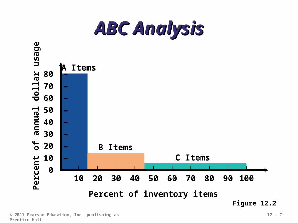
ABC AnalysisABC Analysis

Divides inventory into three classes based on annual dollar volume Class A - high annual dollar volume

Class B - medium annual dollar volume

Class C - low annual dollar volume

Used to focus on the few critical parts (A) and not the many trivial ones (C )


ABC AnalysisABC AnalysisItem

Stock Number

Percent of Number of

Items Stocked

Annual Volume (units) x

Unit Cost =

Annual Dollar

Volume

Percent of Annual Dollar

Volume Class

#10286 20% 1,000 $ 90.00 $ 90,000 38.8% A

#11526 500 154.00 77,000 33.2% A

#12760 1,550 17.00 26,350 11.3% B

#10867 30% 350 42.86 15,001 6.4% B

#10500 1,000 12.50 12,500 5.4% B

72%

23%



Item Stock

Number

Percent of Number of

Items Stocked

Annual Volume (units) x

Unit Cost =

Annual Dollar

Volume

Percent of Annual Dollar

Volume Class

#12572 600 $ 14.17 $ 8,502 3.7% C

#14075 2,000 .60 1,200 .5% C

#01036 50% 100 8.50 850 .4% C

#01307 1,200 .42 504 .2% C

#10572 250 .60 150 .1% C

8,550 $232,057 100.0%

5%


C Items


A Items

B Items

Pe

rce

nt

of

an

nu

al d

olla

r u

sa

ge

80 –

70 –

60 –

50 –

40 –

30 –

20 –

10 –

0 – | | | | | | | | | |

10 20 30 40 50 60 70 80 90 100

Percent of inventory itemsFigure 12.2



Policies from this may include More emphasis on supplier development for

A items

Tighter physical inventory control for A items

More care in forecasting A items


Control of Service Control of Service InventoriesInventories

Can be a critical component of profitability

Losses may come from shrinkage or pilferage

Applicable techniques include

1. Good personnel selection, training, and discipline

2. Tight control on incoming shipments

3. Effective control on all goods leaving facility

12 - 11

Models of Inventory ControlModels of Inventory Control

Fixed Quantity Same quantity is ordered each time

the reorder level is reached.

Fixed Period The order is placed at regular times,

but quantity varies according to demand at order time.

© 2011 Pearson Education, Inc. publishing as Prentice Hall


Holding, Ordering, and Holding, Ordering, and Setup CostsSetup Costs

Holding costsHolding costs - the costs of holding or “carrying” inventory over time

Ordering costsOrdering costs - the costs of placing an order and receiving goods

Setup costsSetup costs - cost to prepare a machine or process for manufacturing an order


Inventory Decision ModelsInventory Decision Models

1. Basic economic order quantity (EOQ)

2. Production order quantity (POQ)

3. Fixed period system (FPS)


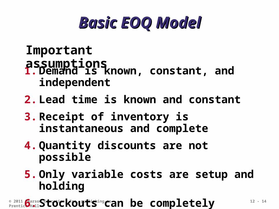
Basic EOQ ModelBasic EOQ Model

1. Demand is known, constant, and independent

2. Lead time is known and constant

3. Receipt of inventory is instantaneous and complete

4. Quantity discounts are not possible

5. Only variable costs are setup and holding

6. Stockouts can be completely avoided

Important assumptions


Inventory Usage Over TimeInventory Usage Over Time

Figure 12.3

Order quantity = Q (maximum inventory

level)

Usage rate Average inventory on hand

Q2

Minimum inventory

Inve

nto

ry le

vel

Time0


Minimizing CostsMinimizing CostsObjective is to minimize total costs

Table 12.4(c)

An

nu

al c

ost

Order quantity

Total cost of holding and setup (order)

Holding cost

Setup (or order) cost

Minimum total cost

Optimal order quantity (Q*)


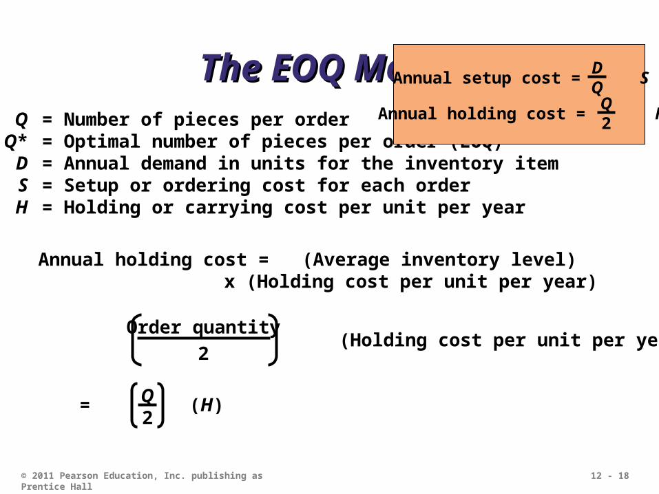
The EOQ ModelThe EOQ ModelQ = Number of pieces per order

Q* = Optimal number of pieces per order (EOQ)D = Annual demand in units for the inventory itemS = Setup or ordering cost for each orderH = Holding or carrying cost per unit per year

Annual setup cost = (Number of orders placed per year) x (Setup or order cost per order)

Annual demand

Number of units in each orderSetup or order cost per order

=

Annual setup cost = SDQ

= (S)DQ




Annual holding cost = (Average inventory level) x (Holding cost per unit per year)

Order quantity

2= (Holding cost per unit per year)

= (H)Q2


Annual holding cost = HQ2




Optimal order quantity is found when annual setup cost equals annual holding cost


Annual holding cost = HQ2

DQ

S = HQ2

Solving for Q*2DS = Q2HQ2 = 2DS/H

Q* = 2DS/H


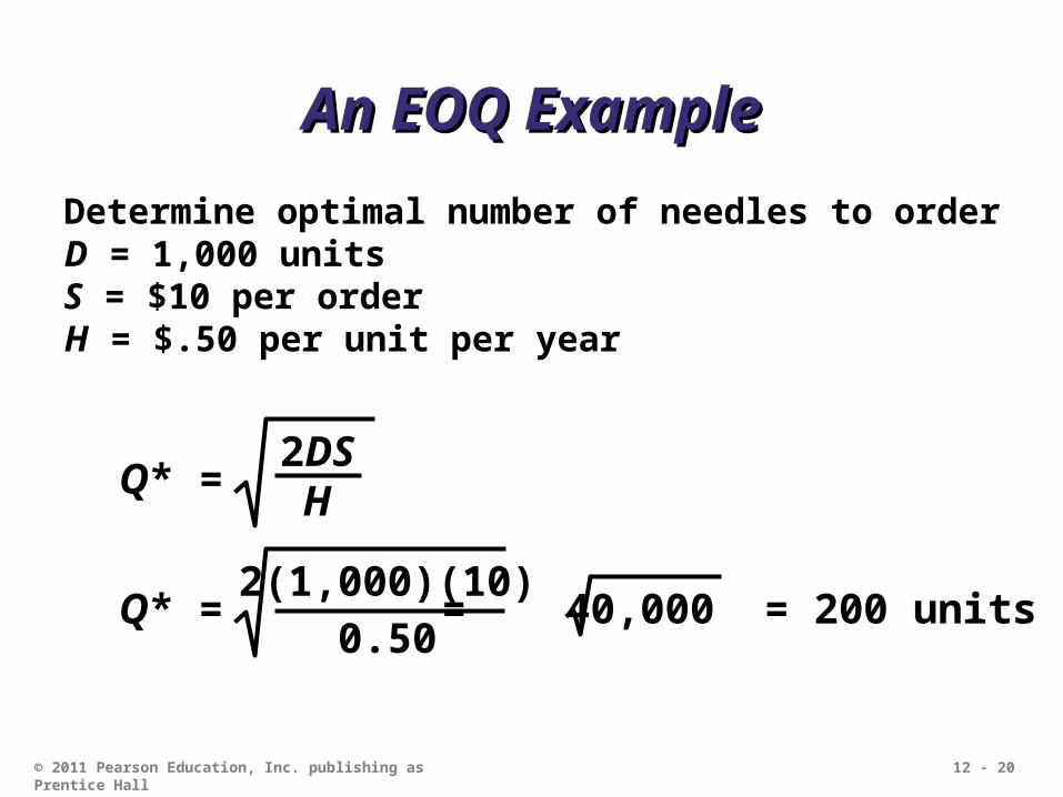
An EOQ ExampleAn EOQ Example

Determine optimal number of needles to orderD = 1,000 unitsS = $10 per orderH = $.50 per unit per year

Q* =2DS

H

Q* =2(1,000)(10)

0.50= 40,000 = 200 units



Determine optimal number of needles to orderD = 1,000 units Q* = 200 unitsS = $10 per orderH = $.50 per unit per year

= N = =Expected number of

orders

DemandOrder quantity

DQ*

N = = 5 orders per year 1,000200



Determine optimal number of needles to orderD = 1,000 units Q* = 200 unitsS = $10 per order N = 5 orders per yearH = $.50 per unit per year

= T =Expected

time between orders

Number of working days per year

N

T = = 50 days between orders250

5



Determine optimal number of needles to orderD = 1,000 units Q* = 200 unitsS = $10 per order N = 5 orders per yearH = $.50 per unit per year T = 50 days

Total annual cost = Setup cost + Holding cost

TC = S + HDQ

Q2

TC = ($10) + ($.50)1,000200

2002

TC = (5)($10) + (100)($.50) = $50 + $50 = $100


Robust ModelRobust Model

The EOQ model is robust

It works even if all parameters and assumptions are not met

The total cost curve is relatively flat in the area of the EOQ



Management underestimated demand by 50%D = 1,000 units Q* = 200 unitsS = $10 per order N = 5 orders per yearH = $.50 per unit per year T = 50 days

TC = S + HDQ

Q2

TC = ($10) + ($.50) = $75 + $50 = $1251,500200

2002

1,500 units

Total annual cost increases by only 25%



Actual EOQ for new demand is 244.9 unitsD = 1,000 units Q* = 244.9 unitsS = $10 per order N = 5 orders per yearH = $.50 per unit per year T = 50 days

TC = S + HDQ

Q2

TC = ($10) + ($.50)1,500244.9

244.92

1,500 units

TC = $61.24 + $61.24 = $122.48

Only 2% less than the total cost of $125

when the order quantity

was 200


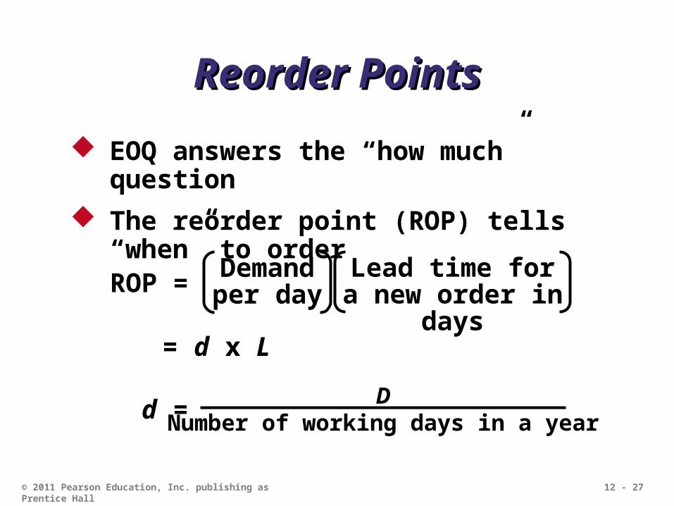
Reorder PointsReorder Points

EOQ answers the “how much” question

The reorder point (ROP) tells “when” to order

ROP =Lead time for a

new order in daysDemand per day

= d x L

d = D

Number of working days in a year


Reorder Point CurveReorder Point Curve

Q*

ROP (units)In

ven

tory

lev

el (

un

its)

Time (days)

Figure 12.5 Lead time = L

Slope = units/day = d

Resupply takes place as order arrives


Reorder Point ExampleReorder Point Example

Demand = 8,000 iPods per year250 working day yearLead time for orders is 3 working days

ROP = d x L

d = D

Number of working days in a year

= 8,000/250 = 32 units

= 32 units per day x 3 days = 96 units


Production Order Quantity Production Order Quantity ModelModel

Used when inventory builds up over a period of time after an order is placed

Used when units are produced and sold simultaneously



Inve

nto

ry l

evel

Time

Demand part of cycle with no production

Part of inventory cycle during which production (and usage) is taking place

t

Maximum inventory

Figure 12.6



Q = Number of pieces per order p = Daily production rateH = Holding cost per unit per year d = Daily demand/usage ratet = Length of the production run in days

= (Average inventory level) xAnnual inventory holding cost

Holding cost per unit per year

= (Maximum inventory level)/2Annual inventory level

= –Maximum inventory level

Total produced during the production run

Total used during the production run

= pt – dt



Q = Number of pieces per order p = Daily production rateH = Holding cost per unit per year d = Daily demand/usage ratet = Length of the production run in days

= –Maximum inventory level

Total produced during the production run

Total used during the production run

= pt – dt

However, Q = total produced = pt ; thus t = Q/p

Maximum inventory level = p – d = Q 1 –

Qp

Qp

dp

Holding cost = (H) = 1 – H dp

Q2

Maximum inventory level2



Q = Number of pieces per order p = Daily production rateH = Holding cost per unit per year d = Daily demand/usage rateD = Annual demand

Q2 =2DS

H[1 - (d/p)]

Q* =2DS

H[1 - (d/p)]p

Setup cost = (D/Q)S

Holding cost = HQ[1 - (d/p)]12

(D/Q)S = HQ[1 - (d/p)]12


Production Order Quantity Production Order Quantity ExampleExample

D = 1,000 units p = 8 units per dayS = $10 d = 4 units per dayH = $0.50 per unit per year

Q* =2DS

H[1 - (d/p)]

= 282.8 or 283 hubcaps

Q* = = 80,0002(1,000)(10)

0.50[1 - (4/8)]



When annual data are used the equation becomes

Q* =2DS

annual demand rateannual production rate

H 1 –

Note:

d = 4 = =D

Number of days the plant is in operation

1,000

250

12 - 38

Fixed Period System ModelFixed Period System Model

Inventory level checked at fixed times.

Order placed to bring level up to maximum.

Can use EOQ to find best time period, by

T = Q* / D (time period = EOQ / demand)


12 - 39

FPS Maximum Inventory LevelFPS Maximum Inventory Level

M = d (T+ L)

Maximum = average demand (Time period + lead time)


12 - 40

FPS Order Size FPS Order Size

Qt = M - IPt

Quantity (at ‘t’) = maximum- inventory (at ‘t’)


12 - 1© 2011 pearson education, inc. publishing as prentice hall importance of inventory one of the...

Documents