11627444.pdfan application of multistate reliability theory to an offshore gas pipeline network

November 13, 2003 11:9 WSPC/122-IJRQSE 00121

International Journal of Reliability, Quality and Safety EngineeringVol. 10, No. 4 (2003) 361–381c© World Scientific Publishing Company

AN APPLICATION OF MULTISTATE RELIABILITY THEORY

TO AN OFFSHORE GAS PIPELINE NETWORK

BENT NATVIG

Department of Mathematics, University of Oslo,

P. O. Box 1053 Blindern, N-0316 Oslo, Norway

[email protected]

HANS W. H. MØRCH

Faculty of Education, Oslo University College,

Pilestredet 52, N-0167 Oslo, Norway

[email protected]

Received 10 December 2002Revised 20 May 2003

The basic multistate reliability theory was developed in the eighties and the beginning ofthe nineties, replacing traditional reliability theory where the system and the componentsare always described as functioning or failed. In Natvig et al.10 the theory was applied toan electrical power generation system for two nearby oilrigs, where the amounts of powerthat may possibly be supplied to the two oilrigs are considered as system states. However,there is still a need for several convincing case studies demonstrating the practicabilityof the generalizations introduced. In the present paper the theory is applied to theNorwegian offshore gas pipeline network in the North Sea, as of the end of the eighties,

transporting gas to Emden in Germany. The system state depends on the amount of gasactually delivered, but also to some extent on the amount of gas compressed mainly bythe compressor component closest to Emden.

Keywords: Availabilities; unavailabilities.

1. Introduction and Basic Definitions

The basic multistate reliability theory was developed in the eighties and the be-

ginning of the nineties, replacing traditional reliability theory where the system

and the components are always described as functioning or failed. A review of the

early development in this area is given in Natvig.8 In Natvig et al.10 the theory was

applied to an electrical power generation system for two nearby oilrigs, where the

amounts of power that may possibly be supplied to the two oilrigs are considered as

system states. However, more than fifteen years later, there is still a need for sev-

eral convincing case studies demonstrating the practicability of the generalizations

introduced. In the present paper the theory is applied to the Norwegian offshore

gas pipeline network in the North Sea, as of the end of the eighties, transporting

361


362 B. Natvig & H. W. H. Mørch

gas to Emden in Germany. The system state depends on the amount of gas actually

delivered, but also to some extent on the amount of gas compressed mainly by the

compressor component closest to Emden.

Let S = {0, 1, . . . , M} be the set of states of the system; the M + 1 states

representing successive levels of performance ranging from the perfect functioning

level M down to the complete failure level 0. Furthermore, let C = {1, . . . , n} be

the set of components and Si (i = 1, . . . , n) the set of states of the ith component.

We claim {0, M} ⊆ Si ⊆ S. Hence, the states 0 and M are chosen to represent the

endpoints of a performance scale that might be used for both the system and its

components. Let xi (i = 1, . . . , n) denote the state or performance level of the ith

component and x = (x1, . . . , xn). It is assumed that the state, φ, of the system is

given by the structure function φ = φ(x). In this paper we consider the following

type of multistate systems for which a series of results can be derived.

Definition 1. A system is a multistate monotone system (MMS) iff its structure

φ satisfies:

(i) φ(x) is non-decreasing in each argument

(ii) φ(0) = 0 and φ(M) = M (0 = (0, . . . , 0), M = (M, . . . , M)).

The first assumption roughly says that improving one of the components cannot

harm the system, whereas the second says that if all components are in the complete

failure (perfect functioning) state, then the system is in the complete failure (perfect

functioning) state.

In what follows y < x means yi ≤ xi for i = 1, . . . , n, and yi < xi for some i.

Definition 2. Let φ be the structure function of an MMS and let j ∈ {1, . . . , M}.

A vector x is said to be a minimal path (cut) vector to level j iff φ(x) ≥ j and

φ(y) < j for all y < x (φ(x) < j and φ(y) ≥ j for all y > x).

Definition 3. The performance process of the ith component (i = 1, . . . , n) is a

stochastic process {Xi(t), t ∈ [0,∞)}, where for each fixed t ∈ [0,∞) Xi(t) is a ran-

dom variable which takes values in Si. The joint performance process for the com-

ponents {X(t), t ∈ [0,∞)} = {(X1(t), . . . , Xn(t)), t ∈ [0,∞)} is the corresponding

vector stochastic process. The performance process of an MMS with structure func-

tion φ is a stochastic process {φ(X(t)), t ∈ [0,∞)}, where for each fixed t ∈ [0,∞),

φ(X(t)) is a random variable which takes values in S.

Definition 4. The performance processes {Xi(t), t ∈ [0,∞)}, i = 1, . . . , n are

independent in the time interval I iff, for any integer m and {t1, . . . , tm} ⊂ I the

random vectors {X1(t1), . . . , X1(tm)}, . . . , {Xn(t1), . . . , Xn(tm)} are independent.

Definition 5. Let j ∈ {1, . . . , M}. The availability, hj(I)φ and the unavailability,

gj(I)φ to level j in the time interval I for an MMS with structure function φ are

given by

hj(I)φ = P [φ(X(s)) ≥ j ∀ s ∈ I ] , g

j(I)φ = P [φ(X(s)) < j ∀ s ∈ I ] .


An Application of Multistate Reliability Theory 363

Note that hj(I)φ + g

j(I)φ ≤ 1, with equality for the case I = [t, t]. In Funnemark

and Natvig3 and Natvig9 bounds for hj(I)φ and g

j(I)φ are arrived at, based on corre-

sponding information on the multistate components, generalizing bounds given in

Natvig7 for the case M = 1. The components are assumed to be maintained and

interdependent. In Natvig11 sufficient conditions are given for some of these bounds

to be strict, and also exact, contributing to the understanding of the nature of the

bounds and to their applicability. It is the aim of this paper to give such bounds

for our offshore gas pipeline network.

In the latter paper it is also shown that for the case where the performance

processes of the components are independent in I , no additional assumption that

each of these is associated in I , is needed to establish any strict or non-strict bounds.

Neither Esary and Proschan2 and Natvig7 treating the binary case nor Fun-

nemark and Natvig3 and Natvig9 treating the multistate case were aware of this.

Accordingly, this was not taken into account in the case study considered in Natvig

et al.,10 but it is in the present paper.

2. An Offshore Gas Pipeline Network

The offshore gas pipeline network treated in this paper is the most complex of

the ones considered in Mørch.6 It constitutes the main parts of the network in the

North Sea, as of the end of the eighties, transporting gas to Emden in Germany. The

network along with its modules are given in Fig. 1. As can be seen from this figure

the network consists altogether of 32 components and 7 non-trivial modules. a1 and

a2 are pipelines from the production field at Statfjord, c1 from the Heimdal and

Troll fields, c2 from the Sleipner field and finally e from the Ekofisk field. All these oil

b d

e

f

g

h

i

j

k

a1

a2

c1

c2

Pf (45) Ph (50) Pj (50)

Pb4 (4.2) Pb5 (8) Pb6 (10.3)

b1 b2 b3 b4 b5 b6 b7 b8

b

d1 d2 d3 d4 d5 d6

d

f1 f2

f

h1 h2

h

j1 j2

j

i1 i2

i

Pi2 (30)

Pd2 (35) Pd6 (30)

Pg4 (30)

g

g1 g2 g3 g4

Fig. 1. Gas pipeline network with corresponding modules b, d, f , g, h, i, j.



and gas fields are in the Norwegian sector of the North Sea west of southern Norway.

k is the pipeline from what is called H7 to Emden. The compressor components of

the network are f1, h1 and j1.

There are 10 passages in the network all supposed to function perfectly. For

instance, Pf (45) is the passage of module f having a capacity of 45 MSm3/d (million

standard cubic metres per day). Similarly, Pb4(4.2) is the passage of component b4

having a capacity of 4.2 MSm3/d. The module passages Pf , Ph and Pj are used

whenever the corresponding modules cannot transport and compress the incoming

amounts of gas, by transporting, within their capacities, the surplus amount of gas.

The 7 component passages are only used when the corresponding components are

not in the perfect functioning state, chosen somewhat arbitrarily to be M = 16.

The gas pipeline from Ekofisk to Emden being part of this network is called

Norpipe. Today there are two more pipelines, Europipe 1 and Europipe 2, providing

Norwegian offshore gas to Emden. In addition Zeepipe provides gas to Zeebrugge

in Belgium and Franpipe gas to Dunkerque in France. Hence, the total Norwegian

offshore gas pipeline network of today is more complex than the one considered in

the present paper.

Let us look closer at the compressor components and start with f1. f1 consists of

four compressors each with a capacity of transporting and compressing 11 MSm3/d.

The states of f1 are defined in Table 1. Since the expected maintenance time for

a compressor is assumed longer than the expected repair time, it is seen from the

table that a failed compressor leads to a higher component state than a maintained

one. Furthermore, we assume that at most three compressors can be used at the

same time implying that the maximum capacity of f1 is 33 MSm3/d, which is

achieved when the component state is 14, 15 or 16. The compressor components h1

and j1 both consists of three compressors each with a capacity of transporting and

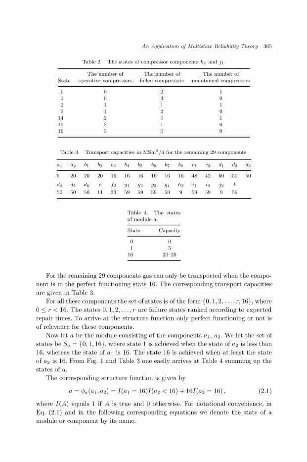
compressing 4.5 MSm3/d. The states of h1 and j1 are defined in Table 2.

Now at most two compressors can be used at the same time implying that the

maximum capacity of both h1 and j1 is 9 MSm3/d, which is achieved when the

component state is 14, 15 or 16.

Table 1. The states of compressor component f1.

The number of The number of The number ofState operative compressors failed compressors maintained compressors

0 0 3 11 0 4 02 1 2 13 1 3 04 2 1 15 2 2 0

14 3 0 115 3 1 016 4 0 0



Table 2. The states of compressor components h1 and j1.

The number of The number of The number ofState operative compressors failed compressors maintained compressors

0 0 2 11 0 3 02 1 1 13 1 2 0

14 2 0 115 2 1 016 3 0 0

Table 3. Transport capacities in MSm3/d for the remaining 29 components.

a1 a2 b1 b2 b3 b4 b5 b6 b7 b8 c1 c2 d1 d2 d3

5 20 20 20 16 16 16 16 16 16 48 42 50 50 50

d4 d5 d6 e f2 g1 g2 g3 g4 h2 i1 i2 j2 k

50 50 50 11 33 59 59 59 59 9 59 59 9 59

Table 4. The statesof module a.

State Capacity

0 01 5

16 20–25

For the remaining 29 components gas can only be transported when the compo-

nent is in the perfect functioning state 16. The corresponding transport capacities

are given in Table 3.

For all these components the set of states is of the form {0, 1, 2, . . . , r, 16}, where

0 ≤ r < 16. The states 0, 1, 2, . . . , r are failure states ranked according to expected

repair times. To arrive at the structure function only perfect functioning or not is

of relevance for these components.

Now let a be the module consisting of the components a1, a2. We let the set of

states be Sa = {0, 1, 16}, where state 1 is achieved when the state of a2 is less than

16, whereas the state of a1 is 16. The state 16 is achieved when at least the state

of a2 is 16. From Fig. 1 and Table 3 one easily arrives at Table 4 summing up the

states of a.

The corresponding structure function is given by

a = φa(a1, a2) = I(a1 = 16)I(a2 < 16) + 16I(a2 = 16) , (2.1)

where I(A) equals 1 if A is true and 0 otherwise. For notational convenience, in

Eq. (2.1) and in the following corresponding equations we denote the state of a

module or component by its name.



Table 5. The states

of module b.

State Capacity

0 01 4.22 8.03 10.3

16 16

Table 6. The statesof module ab.

State Capacity

0 01 4.22 53 8.04 10.3

16 16

From Fig. 1 and Table 3 one gets Table 5 summing up the states of module b.


b = φb(b1, b2, b3, b4, b5, b6, b7, b8)

= I(min(b1, b2, b3, b7, b8) = 16){I(b4 < 16)

+ I(b4 = 16)[2 + I(b5 = 16)[1 + 13I(b6 = 16)]]} . (2.2)

Combining the modules a and b into module ab, from Tables 4 and 5 one arrives

at Table 6 summing up the states of this module.


ab = φab(a, b) = I(min(a, b) > 0)

×{I(a = 1)[1 + I(b ≥ 2)] + I(a = 16)[I(b = 1)

+ 3I(b = 2) + 4I(b = 3) + 16I(b = 16)]} . (2.3)

Let c be the module consisting of the components c1 and c2. We let the set of

states be Sc = {0, 6, 7, 16}. Here state 6 is achieved when the state of c1 is less

than 16, whereas the state of c2 is 16. The state 7 is achieved when it is the other

way round, whereas the state 16 is achieved when both the state of c1 and c2 is 16.

From Fig. 1 and Table 3 one gets Table 7 summing up the states of c.


c = φc(c1, c2) = 6I(c1 < 16)I(c2 = 16) + 7I(c1 = 16)I(c2 < 16)

+ 16I(c1 = 16)I(c2 = 16) . (2.4)



Table 7. The states

of module c.

State Capacity

0 06 427 48

16 90

Table 8. The statesof module d.

State Capacity

0 03 304 35

16 50

Table 9. The statesof module abcde.

State Capacity

0 01 4.2–192 21.3–273 304 355 41–427 46–488 50–53

16 57.2–61

From Fig. 1 and Table 3 one arrives at Table 8 summing up the states of module

d.


d = φd(d1, d2, d3, d4, d5, d6) = I(min(d1, d3, d4, d5) = 16)

×{3 + I(d2 < 16)I(d6 = 16) + 13I(d2 = 16)I(d6 = 16)} . (2.5)

Combining the modules ab, c, d and component e into module abcde, from Fig. 1

and Tables 3, 6, 7, 8 one gets Table 9 summing up the states of module abcde.


abcde = φabcde(ab, c, d, e)

= I(d = 0)I(e = 16) + I(d = 3){I(c = 0)

× [I(e < 16)I(ab > 0) + I(e = 16)(I(ab < 4) + 2I(ab ≥ 4))]

+ I(c > 0)[3 + 2I(e = 16)]}+ I(d = 4){I(c = 0)



Table 10. The states of module f .

State Capacity/Compression

0 02 114 22

16 33

Table 11. The states of modules hand j.

State Capacity/Compression

0 01 4.5

16 9

× [I(e < 16)I(ab > 0) + I(e = 16)(I(ab < 4) + 2I(ab ≥ 4))]

+ I(c > 0)[4 + 3I(e = 16)]} + I(d = 16){I(c = 0)

× [I(e < 16)I(ab > 0) + I(e = 16)(I(ab < 4) + 2I(ab ≥ 4))]

+ I(c = 6)[5 + I(e < 16)(2I(1 ≤ ab ≤ 2) + 3I(ab ≥ 3))

+ I(e = 16)(3 + 8I(ab ≥ 1))] + I(c = 7)[7

+ I(e < 16)I(ab > 0) + 9I(e = 16)] + I(c = 16)[8 + 8I(e = 16)]} . (2.6)

From Fig. 1 and Tables 1, 3 one arrives at Table 10 summing up the states of

module f .


f = φf (f1, f2) = I(f2 = 16)[2I(2 ≤ f1 ≤ 3)

+ 4I(4 ≤ f1 ≤ 5) + 16I(14 ≤ f1 ≤ 16)] . (2.7)

Similarly, from Fig. 1 and Tables 2, 3 we obtain Table 11 summing up the states of

modules h and j.

The corresponding structure functions are given by

h = φh(h1, h2) = I(h2 = 16)[I(2 ≤ h1 ≤ 3) + 16I(14 ≤ h1 ≤ 16)] (2.8)

j = φj(j1, j2) = I(j2 = 16)[I(2 ≤ j1 ≤ 3) + 16I(14 ≤ j1 ≤ 16)] . (2.9)

From Fig. 1 and Table 3 we arrive at Table 12 summing up the states of modules

g and i.

The corresponding structure functions are given by

g = φg(g1, g2, g3, g4) = I(min(g1, g2, g3) = 16)[3 + 13I(g4 = 16)] (2.10)

i = φi(i1, i2) = I(i1 = 16)[3 + 13I(i2 = 16)] . (2.11)



Table 12. The states

of modules g and i.

State Capacity

0 03 30

16 59

Table 13. System states.

State Capacity Compression

0 0 –1 4.2–19 –2 21.3–27 –3 30 –4 35 –5 41–42 –6 45 –7 46–48 –8 50 09 50–53 4.5

10 50–53 911 50–53 9+

12 54.5 4.513 54.5 9

14 56 915 57.2–59 916 57.2–59 9+

At last we are in the position of considering the system as a whole. From Fig. 1

and Tables 9–12 we obtain Table 13 summing up the system states. In this table

mainly the amount of gas compressed by module j, being closest to Emden, is taken

into account, but only when the amount of transported gas is at least 50 MSm3/d.

In addition a “+” in the compression column indicates the advantageous situation

where all compressor modules f , h and j are in state 16. Of course this simplifying

approach is not necessary, but as is seen, even this approach leads to a rather

complex system structure function.

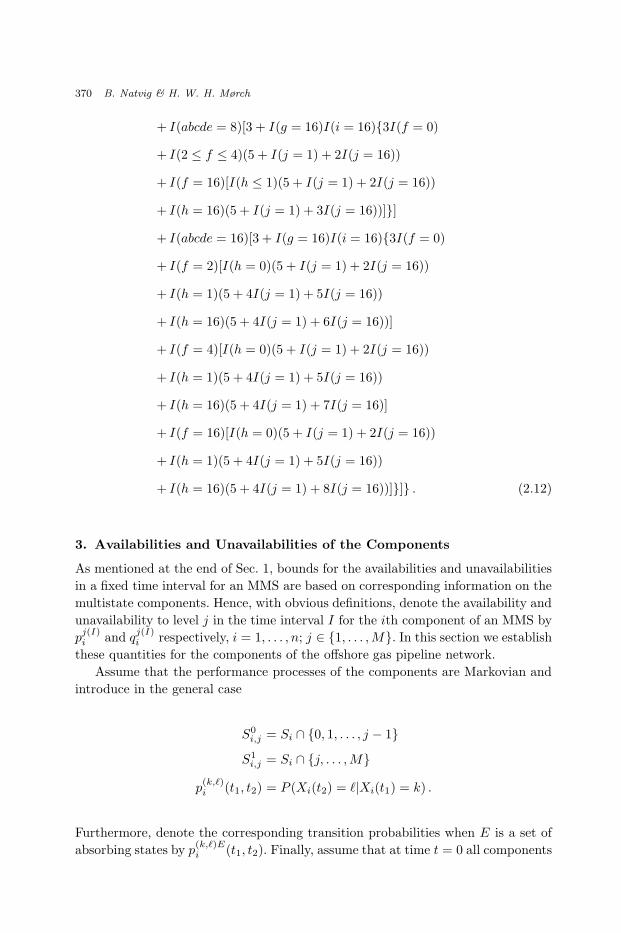
Some careful thinking leads to the following system structure function

φ(abcde, f, g, h, i, j, k)

= I(k = 16)I(min(abcde, g, i) > 0)

×{I(abcde ≤ 3)abcde + I(abcde = 4)[3 + I(g = 16)I(i = 16)]

+ I(abcde = 5)[3 + 2I(g = 16)I(i = 16)]

+ I(abcde = 7)[3 + I(g = 16)I(i = 16)(3I(f = 0) + 4I(f > 0))]



+ I(abcde = 8)[3 + I(g = 16)I(i = 16){3I(f = 0)

+ I(2 ≤ f ≤ 4)(5 + I(j = 1) + 2I(j = 16))

+ I(f = 16)[I(h ≤ 1)(5 + I(j = 1) + 2I(j = 16))

+ I(h = 16)(5 + I(j = 1) + 3I(j = 16))]}]

+ I(abcde = 16)[3 + I(g = 16)I(i = 16){3I(f = 0)

+ I(f = 2)[I(h = 0)(5 + I(j = 1) + 2I(j = 16))

+ I(h = 1)(5 + 4I(j = 1) + 5I(j = 16))

+ I(h = 16)(5 + 4I(j = 1) + 6I(j = 16))]

+ I(f = 4)[I(h = 0)(5 + I(j = 1) + 2I(j = 16))

+ I(h = 1)(5 + 4I(j = 1) + 5I(j = 16))

+ I(h = 16)(5 + 4I(j = 1) + 7I(j = 16)]

+ I(f = 16)[I(h = 0)(5 + I(j = 1) + 2I(j = 16))

+ I(h = 1)(5 + 4I(j = 1) + 5I(j = 16))

+ I(h = 16)(5 + 4I(j = 1) + 8I(j = 16))]}]} . (2.12)

3. Availabilities and Unavailabilities of the Components

As mentioned at the end of Sec. 1, bounds for the availabilities and unavailabilities

in a fixed time interval for an MMS are based on corresponding information on the

multistate components. Hence, with obvious definitions, denote the availability and

unavailability to level j in the time interval I for the ith component of an MMS by

pj(I)i and q

j(I)i respectively, i = 1, . . . , n; j ∈ {1, . . . , M}. In this section we establish

these quantities for the components of the offshore gas pipeline network.

Assume that the performance processes of the components are Markovian and

introduce in the general case

S0i,j = Si ∩ {0, 1, . . . , j − 1}

S1i,j = Si ∩ {j, . . . , M}

p(k,`)i (t1, t2) = P (Xi(t2) = `|Xi(t1) = k) .

Furthermore, denote the corresponding transition probabilities when E is a set of

absorbing states by p(k,`)Ei (t1, t2). Finally, assume that at time t = 0 all components



are in the perfect functioning state M ; i.e., X(0) = M. Then for I = [t1, t2]

pj(I)i =

∑

k∈S1

i,j

p(M,k)i (0, t1)

1 −∑

`∈S0

i,j

p(k,`)S0

ij

i (t1, t2)

(3.1)

qj(I)i =

∑

k∈S0

i,j

p(M,k)i (0, t1)

1 −∑

`∈S1

i,j

p(k,`)S1

ij

i (t1, t2)

. (3.2)

Note that we get qj(I)i from p

j(I)i by replacing S1

ij by the “dual” set S0ij .

Now let

µ(k,`)i (s) = lim

h→0p(k,`)i (s, s + h)/h , k 6= ` ,

be the transition intensities of {Xi(t), t ∈ [0,∞)}. For simplicity we assume that

the performance processes of the components are time-homogeneous, i.e.

p(k,`)i (t1, t2) = p

(k,`)i (t2 − t1)

µ(k,`)i (s) = µ

(k,`)i for all s ∈ [0,∞), k 6= ` .

Consequently, all that is needed to arrive at expressions for pj(I)i and q

j(I)i , and

hence bounds for hj(I)φ and g

j(I)φ , are these time-independent transition intensities.

Now introduce the matrices

Pi(t) = {p(k,`)i (t)}k∈Si,`∈Si

Since the set Si is finite, the performance processes of the components are con-

servative, implying that the corresponding intensity matrices are on the form

(i = 1, . . . , n)

Ai =

−

M∑

k=1

µ0k · · · µ0M

......

µM0 · · · −

M−1∑

k=0

µMk

Denoting |Si| the cardinality of the set Si, Ai is an |Si| × |Si| matrix.

By applying standard theory for finite-state continuous-time Markov processes,

see Karlin and Taylor,5 we have

Pi(t) = exp(Ai(t)) = I +

∞∑

n=1

Ani tn

n!,

where I is the identity matrix and the initial condition is Pi(0) = I.

The availabilities and unavailabilities of the 32 components of the offshore gas

pipeline system are determined by the computer package MUSTAFA (MUltiSTAte



Fault tree Analysis) developed by Høg̊asen.4 The only input needed are the intensity

matrices of the components, implicitly giving the corresponding sets of states, along

with the time interval I .

The intensity matrices of a1 and the compressor component f1 are given below.

For the interested reader, aiming for instance at checking our results by a simulation

study, the remaining intensity matrices are given in the appendix.

Aa1=

−4 0 0 0 4

0 −8.3721 0 0 8.3721

0 0 −9 0 9

0 0 0 −22.25 22.25

0.00003 0.0019 0.028 0.0061 −0.03603

Note that Sa1= {0, 1, 2, 3, 16}, and that the failure states are ranked according to

inverse repair rates or, equivalently, the expected repair times.

Af1

=

−1783.35 0 1711.35 72 0 0 0 0 0

0 −2281.8 0 2281.8 0 0 0 0 0

9.6 0 −1222.5 0 1140.9 72 0 0 0

0 9.6 0 −1720.95 0 1711.35 0 0 0

0 0 19.2 0 −661.7 0 570.45 72 0

0 0 0 19.2 0 −1160.1 0 1140.9 0

0 0 0 0 28.8 0 −100.8 0 72

0 0 0 0 0 28.8 0 −599.25 570.450 0 0 0 0 0 20 38.4 −58.4

Note that the maintenance completion rate of 72 completions per year is smaller

than the repair rate of a single compressor of 570.45 repairs per year as assumed

when ranking the states of f1 in Table 1, and that there are four repairmen. Note

also that a compressor is only sent for maintenance when all four compressors are

operative, and that in this case the fourth compressor is in hot standby.

4. Bounds for the Availabilities and Unavailabilities for the

Offshore Gas Pipeline Network

As an example of the bounds for hj(I)φ and g

j(I)φ given in Funnemark and Natvig3

and Natvig,9 without any assumption according to Natvig11 that each of the perfor-

mance processes of the components is associated in I , we give the following theorem

by first introducing the n × M matrices

P(I)φ =

{

pj(I)i

}

i=1,...,n

j=1,...,M

, Q(I)φ =

{

qj(I)i

}

i=1,...,n

j=1,...,M

.



Theorem 1. Let (C, φ) be an MMS with the marginal performance processes

of its components being independent in I . Furthermore, for j ∈ {1, . . . , M} let

yjk = (yj

1k, . . . , yjnk), k = 1, . . . , nj (zj

k = (zj1k, . . . , zj

nk), k = 1, . . . , mj) be its

minimal path (cut) vectors to level j. Define

`j′

φ (P(I)φ ) = max

1≤k≤nj

n∏

i=1

py

j

ik(I)

i , ¯̀j′

φ (Q(I)φ ) = max

1≤k≤mj

n∏

i=1

qz

j

ik+1(I)

i

`j∗

φ (P(I)φ ) =

mj

∏

k=1

n∐

i=1

pz

j

ik+1(I)

i , ¯̀j∗

φ (Q(I)φ ) =

nj

∏

k=1

n∐

i=1

qy

j

ik(I)

i

Bjφ(P

(I)φ ) = max

j≤k≤M

{

max[`k′

φ (P(I)φ ), `k∗

φ (P(I)φ )]

}

B̄jφ(Q

(I)φ ) = max

1≤k≤j

{

max[¯̀k′

φ (Q(I)φ ), ¯̀k∗

φ (Q(I)φ )]

}

.

Then

Bjφ(P

(I)φ ) ≤ h

j(I)φ ≤ inf

t∈I

[

1 − B̄jφ(Q

([t,t])φ )

]

≤ 1 − B̄jφ(Q

(I)φ )

B̄jφ(Q

(I)φ ) ≤ g

j(I)φ ≤ inf

t∈I

[

1− Bjφ(P

([t,t])φ )

]

≤ 1 − Bjφ(P

(I)φ ) .

Here∐n

i=1 aidef= 1 −

∏n

i=1(1 − ai). By specializing M = 1 and I = [t, t] the

bounds reduce to the familiar ones from binary theory as given in Barlow and

Proschan.1

By using the computer package MUSTAFA, which finds the minimal path and

cut vectors to all levels from Eqs. (2.1)–(2.12) and then applies the best bounds

of Theorem 1, we arrive at the bounds shown in Table 14, which are not based

on a modular decomposition. Note that for the case I = [0.5, 0.5] we know from

Sec. 1 that gj[0.5,0.5]φ = 1−h

j[0.5,0.5]φ . Hence, the bounds for g

j[0.5,0.5]φ follow immedi-

ately from the ones of hj[0.5,0.5]φ . Furthermore, note that the upper bounds both for

hj[0.5,0.6]φ and h

j[0.5,0.5]φ , and also for g

j[0.5,0.6]φ and g

j[0.5,0.5]φ , are almost completely

identical. This is due to the fact that the upper bounds for a fixed time point t in

Theorem 1 do not depend on t for t ≥ 0.5. Hence, stationarity is reached after half

a year. We see that all bounds are very informative for I = [0.5, 0.5] and for the

unavailabilities also for I = [0.5, 0.6], corresponding to an interval length of 36 days.

They are less informative for the availabilities for I = [0.5, 0.6]. Note, however, that

from the theory we know that all lower bounds are far better than the correspond-

ing upper bounds especially for long intervals. Also, to be on the conservative side,

the lower bounds for the availabilities are the most interesting.

It should be remarked that none of the intervals in Table 14 reduce to a single

exact value. This follows from the theory in Natvig11 since there are more than one

single minimal path and minimal cut vector to all levels. Exact values are obtained

in Mørch6 for some simpler networks.



Table 14. Bounds for hj(I)φ

and gj(I)φ

not based on a modulardecomposition.

j I Bounds for hj(I)φ

Bounds for gj(I)φ

Lower Upper Lower Upper

16[0.5, 0.6] 0.0897 0.9600 0.0120 0.0836

[0.5, 0.5] 0.9164 0.9601 0.0399 0.0836

15[0.5, 0.6] 0.1672 0.9600 0.0120 0.0738

[0.5, 0.5] 0.9262 0.9601 0.0399 0.0738

14[0.5, 0.6] 0.1706 0.9600 0.0120 0.0737

[0.5, 0.5] 0.9263 0.9601 0.0399 0.0737

13[0.5, 0.6] 0.2422 0.9600 0.0120 0.0686

[0.5, 0.5] 0.9314 0.9601 0.0399 0.0686

12[0.5, 0.6] 0.3439 0.9600 0.0120 0.0635

[0.5, 0.5] 0.9365 0.9601 0.0399 0.0635

11[0.5, 0.6] 0.3439 0.9968 0.0011 0.0254

[0.5, 0.5] 0.9746 0.9968 0.0032 0.0254

10[0.5, 0.6] 0.3904 0.9968 0.0011 0.0230

[0.5, 0.5] 0.9770 0.9968 0.0032 0.0230

9[0.5, 0.6] 0.4113 0.9968 0.0011 0.0228

[0.5, 0.5] 0.9772 0.9968 0.0032 0.0228

8[0.5, 0.6] 0.4492 0.9968 0.0011 0.0211

[0.5, 0.5] 0.9789 0.9968 0.0032 0.0211

7[0.5, 0.6] 0.4566 0.9968 0.0011 0.0207

[0.5, 0.5] 0.9793 0.9968 0.0032 0.0207

6[0.5, 0.6] 0.4720 0.9968 0.0011 0.0199

[0.5, 0.5] 0.9801 0.9968 0.0032 0.0199

5[0.5, 0.6] 0.4802 0.9968 0.0011 0.0195

[0.5, 0.5] 0.9805 0.9968 0.0032 0.0195

4[0.5, 0.6] 0.4810 0.9968 0.0011 0.0195

[0.5, 0.5] 0.9805 0.9968 0.0032 0.0195

3[0.5, 0.6] 0.4952 0.9968 0.0011 0.0189

[0.5, 0.5] 0.9811 0.9968 0.0032 0.0189

2[0.5, 0.6] 0.4952 0.9968 0.0011 0.0189

[0.5, 0.5] 0.9811 0.9968 0.0032 0.0189

1[0.5, 0.6] 0.7354 0.9975 0.0011 0.0112

[0.5, 0.5] 0.9888 0.9975 0.0025 0.0112

The computer package MUSTAFA can also find a modular decomposition of

a system. Then bounds for the availabilities and unavailabilities for the modules

can be established from the availabilities and unavailabilities of the components.

Furthermore, bounds for the availabilities and unavailabilities of the system can

be established from these bounds for the availabilities and unavailabilities for the

modules. Using this approach we arrive at the best bounds shown in Table 15.



Table 15. Bounds for hj(I)φ

and gj(I)φ

based on a modular decom-position found by MUSTAFA.

j I Bounds for hj(I)φ

Bounds for gj(I)φ

Lower Upper Lower Upper

16[0.5, 0.6] 0.0897 0.9246 0.0148 0.0836

[0.5, 0.5] 0.9164 0.9247 0.0753 0.0836

15[0.5, 0.6] 0.1672 0.9344 0.0148 0.0738

[0.5, 0.5] 0.9262 0.9345 0.0655 0.0738

14[0.5, 0.6] 0.1706 0.9346 0.0148 0.0737

[0.5, 0.5] 0.9263 0.9347 0.0653 0.0737

13[0.5, 0.6] 0.2422 0.9397 0.0148 0.0686

[0.5, 0.5] 0.9314 0.9398 0.0602 0.0686

12[0.5, 0.6] 0.3439 0.9449 0.0148 0.0635

[0.5, 0.5] 0.9365 0.9450 0.0550 0.0635

11[0.5, 0.6] 0.3439 0.9828 0.0034 0.0257

[0.5, 0.5] 0.9743 0.9829 0.0171 0.0257

10[0.5, 0.6] 0.3439 0.9828 0.0034 0.0232

[0.5, 0.5] 0.9768 0.9829 0.0171 0.0232

9[0.5, 0.6] 0.4113 0.9828 0.0034 0.0228

[0.5, 0.5] 0.9772 0.9829 0.0171 0.0228

8[0.5, 0.6] 0.4492 0.9845 0.0033 0.0211

[0.5, 0.5] 0.9789 0.9846 0.0154 0.0211

7[0.5, 0.6] 0.4566 0.9845 0.0033 0.0207

[0.5, 0.5] 0.9793 0.9846 0.0154 0.0207

6[0.5, 0.6] 0.4720 0.9853 0.0033 0.0199

[0.5, 0.5] 0.9801 0.9854 0.0146 0.0199

5[0.5, 0.6] 0.4802 0.9853 0.0033 0.0195

[0.5, 0.5] 0.9805 0.9854 0.0146 0.0195

4[0.5, 0.6] 0.4810 0.9853 0.0033 0.0195

[0.5, 0.5] 0.9805 0.9854 0.0146 0.0195

3[0.5, 0.6] 0.4952 0.9859 0.0033 0.0189

[0.5, 0.5] 0.9811 0.9860 0.0140 0.0189

2[0.5, 0.6] 0.4952 0.9859 0.0033 0.0189

[0.5, 0.5] 0.9811 0.9860 0.0140 0.0189

1[0.5, 0.6] 0.7354 0.9889 0.0027 0.0112

[0.5, 0.5] 0.9888 0.9890 0.0110 0.0112

First note that the comments made on Table 14 are still valid for Table 15.

Secondly, note that the bounds for a fixed time point t = 0.5 are more informative

in Table 15 than in Table 14. This is in accordance with the theory of Funnemark

and Natvig,3 Natvig9 and Natvig.11 The same is also true to some extent for the

interval I = [0.5, 0.6], but this is not true in general. For instance, Table 14 gives

0.3904 ≤ h10[0.5,0.6]φ ≤ 0.9968, whereas Table 15 gives 0.3439 ≤ h

10[0.5,0.6]φ ≤ 0.9828.



Finally, it should be concluded that having the computer package MUSTAFA

more complex systems than the one treated here can be attacked.

Acknowledgments

We are very thankful to senior discipline leader Morten Sørum for providing infor-

mation and knowledge on the offshore gas pipeline network considered, to dr.scient

Gutorm Høg̊asen for patience in answering questions on the computer package

MUSTAFA, and to three referees for a careful reading of the manuscript and con-

structive comments.

Appendix: Remaining Intensity Matrices of the Components

Aa2=

−4 0 0 0 4

0 −8.3721 0 0 8.3721

0 0 −9 0 9

0 0 0 −22.5 22.5

0.00006 0.01565 0.021 0.01736 −0.05406

Ab1 =

−1.8 0 0 0 0 1.8

0 −6.207 0 0 0 6.207

0 0 −7.3469 0 0 7.3469

0 0 0 −8.3721 0 8.3721

0 0 0 0 −9 9

0.000066 0.000072 0.0023 0.0082 0.02 −0.03064

Ab2 =

−22.5 0 0 0 22.5

0 −51.4286 0 0 51.4286

0 0 −444.4444 0 444.4444

0 0 0 −720 720

0.109 0.0008 0.31 0.03 −0.4498

Ab3 =

−3.6735 0 0 0 0 3.6735

0 −51.4286 0 0 0 51.4286

0 0 −120 0 0 120

0 0 0 −180 0 180

0 0 0 0 −360 360

0.00099 0.00017 0.0017 0.05 0.44 −0.49286



Ab4 =

[

−120 120

0.08 −0.08

]

Ab5 =

−18 0 0 0 18

0 −51.4286 0 0 51.4286

0 0 −180 0 180

0 0 0 −360 360

0.0085 0.00089 1.6 1.06 −2.66939

Ab6 =

−180 0 0 180

0 −211.7647 0 211.7647

0 0 −360 360

1.8 1.3 0.08 −3.18

Ab7 =

−7.3469 0 0 0 0 7.3469

0 −8.3721 0 0 0 8.3721

0 0 −22.5 0 0 22.5

0 0 0 −51.4286 0 51.4286

0 0 0 0 −444.4444 444.4444

0.00154 0.00554 0.09402 0.0008 0.176 −0.2779

Ab8 = Ac1=

[

−22.5 22.5

0.009 −0.009

]

Ac2=

−4 0 0 4

0 −8.3721 0 8.3721

0 0 −22.5 22.5

0.00003 0.00636 0.01704 −0.02343

Ad1=

−1 0 0 0 0 0 0 1

0 −1.2 0 0 0 0 0 1.2

0 0 −6 0 0 0 0 6

0 0 0 −12 0 0 0 12

0 0 0 0 −22.5 0 0 22.5

0 0 0 0 0 −360 0 360

0 0 0 0 0 0 −900 900

0.00022 0.0004 0.00031 0.0017 0.009 0.14 1.8 −1.95163



Ad2=

[

−444.4444 444.4444

0.175 −0.175

]

Ad3=

−8.3721 0 8.3721

0 −22.5 22.5

0.01276 0.00004 −0.0128

Ad4=

−22.5 0 0 0 0 22.5

0 −360 0 0 0 360

0 0 −444.4444 0 0 444.4444

0 0 0 −720 0 720

0 0 0 0 −900 900

0.0026 0.0017 0.38 0.06 1.8 −2.2443

Ad5=

−1 0 0 0 0 0 1

0 −1.2 0 0 0 0 1.2

0 0 −2 0 0 0 2

0 0 0 −3 0 0 3

0 0 0 0 −6 0 6

0 0 0 0 0 −12 12

0.00022 0.00022 0.00007 0.00041 0.00036 0.00111 −0.00239

Ad6=

−444.4444 0 444.4444

0 −720 720

0.165 0.02 −0.185

Ae =

[

−12 12

0.5 −0.5

]

Af2=

−12 0 0 12

0 −360 0 360

0 0 −444.4444 444.4444

0.0014 0.008 0.311 −0.3204



Ag1=

−1 0 0 0 0 0 0 0 1

0 −1.2 0 0 0 0 0 0 1.2

0 0 −4 0 0 0 0 0 4

0 0 0 −6 0 0 0 0 6

0 0 0 0 −12 0 0 0 12

0 0 0 0 0 −22.5 0 0 22.5

0 0 0 0 0 0 −444.4444 0 444.4444

0 0 0 0 0 0 0 −720 720

0.00066 0.00026 0.0001 0.00062 0.003 0.008 0.301 0.02 −0.33364

Ag2=

−1 0 0 0 0 1

0 −6 0 0 0 6

0 0 −12 0 0 12

0 0 0 −360 0 360

0 0 0 0 −900 900

0.00007 0.0001 0.0001 0.14 1.8 −1.94027

Ag3= Ai1 =

−2 0 0 0 0 2

0 −6 0 0 0 6

0 0 −8.3721 0 0 8.3721

0 0 0 −22.5 0 22.5

0 0 0 0 −360 360

0.0004 0.0003 0.00506 0.018 0.14 −0.16376

Ag4= Ai2 =

−360 0 0 360

0 −444.4444 0 444.4444

0 0 −720 720

0.008 0.107 0.02 −0.135

Ah1= Aj1 =

−1212.9 0 1140.9 72 0 0 0

0 −1711.35 0 1711.35 0 0 0

9.6 0 −652.05 0 570.45 72 0

0 9.6 0 −1150.5 0 1140.9 0

0 0 19.2 0 −91.2 0 72

0 0 0 19.2 0 −589.65 570.45

0 0 0 0 15 28.8 −43.8



Ah2= Aj2 =

−12 0 0 0 0 12

0 −360 0 0 0 360

0 0 −444.4444 0 0 444.4444

0 0 0 −450 0 450

0 0 0 0 −720 720

0.0014 0.104 0.197 0.18 0.33 −0.8124

Ak =

−8.3721 0 0 8.3721

0 −22.5 0 22.5

0 0 −51.4286 51.4286

0.02088 0.00002 0.00075 −0.02165

References

1. R. E. Barlow and F. Proschan, Statistical Theory of Reliability and Life Testing.

Probability Models, Holt, Rinehart & Winston, New York (1975).2. J. D. Esary and F. Proschan, “A reliability bound for systems of maintained, inter-

dependent components,” J. Amer. Statist. Assoc. 65 (1970), pp. 329–338.3. E. Funnemark and B. Natvig, “Bounds for the availabilities in a fixed time interval

for multistate monotone systems,” Adv. Appl. Prob. 17 (1985), pp. 638–665.4. G. Høg̊asen, MUSTAFA programs for MUltiSTAte Fault-tree Analysis, Ph.D thesis,

University of Oslo (1990).5. S. Karlin and H. M. Taylor, A First Course in Stochastic Processes, 2nd edn. Academic

Press, New York (1975).6. H. W. H. Mørch, An application of multistate reliability theory on an existing network

of gas pipelines, Cand. scient. thesis, University of Oslo (in Norwegian), (1991).7. B. Natvig, “Improved bounds for the availability and unavailability in a fixed time

interval for systems of maintained, interdependent components,” Adv. Appl. Prob. 12

(1980), pp. 200–221.8. B. Natvig, “Multistate coherent systems,” Encyclopedia of Statistical Sciences 5

(1985), pp. 732–735.9. B. Natvig, “Improved upper bounds for the availabilities in a fixed time interval for

multistate monotone systems,” Adv. Appl. Prob. 18 (1986), pp. 577–579.10. B. Natvig, S. Sørmo, A. T. Holen and G. Høg̊asen, “Multistate reliability theory —

A case study,” Adv. Appl. Prob. 18 (1986), pp. 921–932.11. B. Natvig, “Strict and exact bounds for the availabilities in a fixed time interval for

multistate monotone systems,” Scand. J. Statist. 20 (1993), pp. 171–175.

About the Authors

Bent Natvig received a cand. real degree at the University of Oslo in 1970 and a

Ph.D. degree at the University of Sheffield in 1976. He became a senior lecturer

at the Department of Statistics and Insurance Mathematics at the University of

Oslo in 1981 and a full Professor in 1986 with special duties in reliability. From

1990–1993 he served as a dean of the Faculty of Natural Sciences and Mathematics



at the University of Oslo. He was elected member of the International Statistical

Institute in 1997.

Hans W. H. Mørch received his cand.scient degree at the University of Oslo in 1991

and is affiliated with the Oslo University College.

11627444.pdfan application of multistate reliability theory to an offshore gas pipeline network

Documents