1

11. The Least-Squares Criterion

The purpose of Chapters 11-15 is to study the recursive least-squares algorithm in greater detail. Rather than motivate it as a stochastic gradient approximation to a steepest descent method, as was done in Sec. 5.9, the discussion in these chapters will bring forth deeper insights into the nature of the RLS algorithm. In particular, it will be seen in Chapter 12 that RLS is an optimal (as opposed to approximate) solution to a well-defined optimization problem. In addition, the discussion will reveal that RLS is very rich in structure, so much so that many equivalent variants exist. While all these variants are mathematically equivalent, they vary among themselves in computational complexity, performance under finite-precision conditions, and even in modularity and ease of implementation.

11.1 Least-Squares Problem Assume we have available N realizations of the random variables d and u, say,

1,2,1,0 Ndddd , 1210 ,,, Nuuuu ,

where the { d ( i ) } are scalars and the {ui} are 1 x M . Given the { d ( i ) , ui}, and assuming ergodicity, we can approximate the mean-square-error cost by its sample average as

1

0

22 1 N

ii wuid

NwudE

In this way, the optimization problem

2min wudEw

can be replaced by the related problem

1

0

2min

N

ii

wwuid

Vector Formulation Forming the references into an N x 1 vector and the regressors become an N x M matrix

1

1

0

Nd

d

d

y

and

1

1

0

Nu

u

u

H

and the cost function is rewritten based on vectors, matrices and the norm square operator as

2min wHy

w

This is defined as the standard least-squares problem.

2

A summary of the four least-squares variants is provided in Table 11.1 on p. 672.

Their orthogonality conditions are given in Table 11.2.

3

The minimum costs are given in Table 11.3.

4

Matlab Simulations

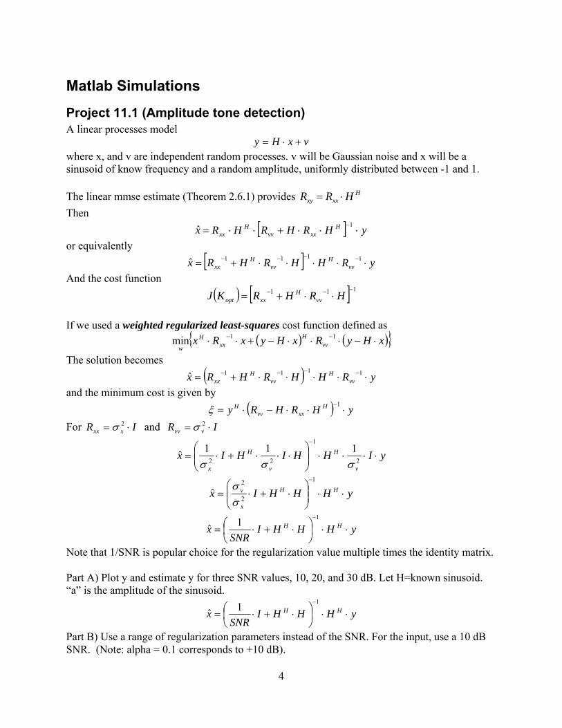
Project 11.1 (Amplitude tone detection) A linear processes model

vxHy where x, and v are independent random processes. v will be Gaussian noise and x will be a sinusoid of know frequency and a random amplitude, uniformly distributed between -1 and 1. The linear mmse estimate (Theorem 2.6.1) provides H

xxxy HRR

Then

yHRHRHRx Hxxvv

Hxx

1ˆ

or equivalently

yRHHRHRx vvH

vvH

xx 1111ˆ

And the cost function

111 HRHRKJ vvH

xxopt

If we used a weighted regularized least-squares cost function defined as

xHyRxHyxRx vvH

xxH

w 11min

The solution becomes

yRHHRHRx vvH

vvH

xx 1111ˆ

and the minimum cost is given by

yHRHRy Hxxvv

H 1

For IR xxx 2 and IR vvv 2

yIHHIHIxv

H

v

H

x

2

1

22

111ˆ

yHHHIx HH

x

v

1

2

2

ˆ

yHHHISNR

x HH

11

ˆ

Note that 1/SNR is popular choice for the regularization value multiple times the identity matrix. Part A) Plot y and estimate y for three SNR values, 10, 20, and 30 dB. Let H=known sinusoid. “a” is the amplitude of the sinusoid.

yHHHISNR

x HH

11

ˆ

Part B) Use a range of regularization parameters instead of the SNR. For the input, use a 10 dB SNR. (Note: alpha = 0.1 corresponds to +10 dB).

5

Project 11.2 (OFDM Receiver) Welcome to advanced communications system signal considerations. Orthogonal-frequency-division multiplexing (OFDM) symbol transmission:

Complex data symbols (QAM-based constellation values) are placed in frequency bins. The data entered is inverse discrete Fourier transformed (generating a real time sequence of fixed length). The time sequence is “circular” in that performing a circular shift on the sequence would only result in additional linear phase in the symbols (if directly discrete Fourier transformed after the circular shift). The last part of the sequence is pre-pended to the front of the sequence (note that any sequence equal to the original length would just provide a linear phase if a DFT were performed). The signal is transmitted. The received signal is truncated to be the exact length of the original DFT, preferably cutting off the cyclic prefix that was prepended. Perform a DFT on the sequence. The “data symbols” are in the DFT bins with some corruption. From the on-line textbook:

6

7

8

9

10

11

12

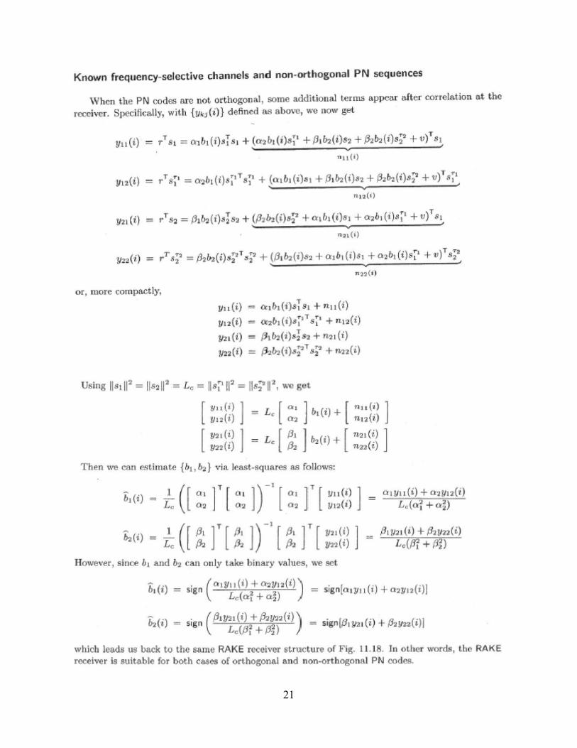
Project 11.3 (CDMA and RAKE Receiver) Welcome to another form of advanced communications with signal processing considerations. Code-division multiple access is a form of direct sequence spread-spectrum communications. A lengthy spreading code (chip sequence) is applied to individual to provide both an encoding that has low correlation (or zero) to all other codes and spreads the spectrum of what otherwise would be narrowband bit level communications. This technique increases signal transmission power across a broad bandwidth while limiting the transmitted power in any narrowband segment. In some application, the spread-spectrum transmission resides below the normal noise spectral power and is not readily observed. Once the correlation gain of the spreading code is used, the signal is coherently combined while noise is non-coherently summed and effectively narrow-band filtered. This coding gain allows the original transmitted power to be restored with sufficient signal-to-noise power ratio for message detection.

13

14

15

16

17

18

19

20

21

22

23

24