100 years of subatomic physics || chiral symmetry in subatomic physics
TRANSCRIPT
May 9, 2013 10:7 World Scientific Review Volume - 9.75in x 6.5in chiral
Chapter 8
Chiral Symmetry in Subatomic Physics
ULF-G. MEIßNER
Helmholtz-Institut fur Strahlen- und Kernphysik
and Bethe Center for Theoretical Physics
Universitat Bonn, D-53115 Bonn, Germany
and
Institut fur Kernphysik, Institute for Advanced Simulation
and Julich Center for Hadron Physics
Forschungszentrum Julich, D-52425 Julich, Germany
These are some personal thoughts on the role of chiral symmetry in subatomic
physics.
1. Introduction
Symmetries play an important role in our understanding of subatomic physics.
Remarkably, the most important consequences are related to the violation of sym-
metries such as the breaking of CP invariance which is a necessary ingredient in the
generation of the observed matter–antimatter asymmetry in the universe. For the
strong interactions, chiral symmetry has always played a prominent role. That be-
came even more important when appropriate effective field theories were developed
that allowed one to systematically work out the strictures of the spontaneous and
explicit broken chiral symmetry of Quantum Chromodynamics (QCD), the gauge
theory that describes the strong interactions on a microscopic basis. In this con-
tribution, I will discuss the role of chiral symmetry in particle and nuclear physics
and, in particular, show how these seemingly separate fields are strongly linked as
QCD generates various forms of strongly interacting matter — the hadrons and
nuclei. Here, the pions which are the Goldstone bosons of the spontaneously bro-
ken chiral symmetry, play a special role as they have profound influences on the
structure and dynamics of hadrons and also the forces between nucleons. When
the pion was predicted by Yukawa in 1935 as the force carrier of the strong interac-
tions, it could hardly be foreseen that almost a century later a systematic theory of
hadron and nuclear interactions could be formulated in which the pion is one of the
main ingredients. Such line of thought started long before QCD as chiral symmetry
has played an important role in shaping our understanding of strong interaction
199
100
Yea
rs o
f Su
bato
mic
Phy
sics
Dow
nloa
ded
from
ww
w.w
orld
scie
ntif
ic.c
omby
MO
NA
SH U
NIV
ER
SIT
Y o
n 08
/29/
13. F
or p
erso
nal u
se o
nly.

May 9, 2013 10:7 World Scientific Review Volume - 9.75in x 6.5in chiral
200 Ulf-G. Meißner
physics. The heydays of current algebra, soft pion theorems and attempts to go
beyond in the 1960s led to a cornucopia of interesting predictions. However, at that
time many of these could hardly be tested and field theory was no longer consid-
ered the appropriate tool for a microscopic theory of the strong interactions. This
changed with the formulation of QCD and the experimental findings of the proton
substructure, leading to new directions in subatomic physics. However, with the
advent of effective field theories and their applications to QCD spear-headed by
Weinberg1 and Gasser and Leutwyler,2,3 a whole new world of precision physics at
low energies opened up — something that many believed could never be achieved
or at most be realized using numerical simulations only. In this contribution, I try
to convey the fascination of working in this challenging field. I will also argue that
the combination of chiral symmetry with other methods such as dispersion relations
or lattice simulations is one of the main directions to further elucidate the role of
chiral symmetry.
This contribution is organized as follows: Section 2 contains a very basic in-
troduction into chiral symmetry, followed by a short discussion of chiral symmetry
breaking and its consequences in Section 3. Chiral symmetry and its realization in
QCD is discussed in Section 4. This is followed by an introduction to the concepts
and foundations of chiral perturbation theory, see Section 5. Then, applications of
chiral perturbations theory and its various extensions are discussed in the following
sections, including pion–pion scattering (Section 6), the role of strange quarks and
pion–kaon scattering (Section 7), the pion cloud of the nucleon (Section 8), meson–
baryon three flavor chiral dynamics, in particular (anti)kaon–nucleon scattering, in
Section 9, and then the role of chiral symmetry in nuclear forces and atomic nuclei
in Section 10. Section 11 is devoted to a short discussion of chiral symmetry in
heavy hadron physics. Some final remarks are collected in Section 12.
2. Chiral Symmetry
In this section, I briefly introduce the concept of chiral symmetry. We consider a
theory of massless fermions, given by the Lagrangian
L = iψγµ∂µψ . (1)
Such a theory possesses a chiral symmetry. To see this, perform a left/right (L/R)-
decomposition of the spin-1/2 field
ψ =1
2(1− γ5)ψ +
1
2(1 + γ5)ψ = PLψ + PRψ = ψL + ψR , (2)
using the projection operators PL/R, that obey P 2
L = PL, P2
R = PR, PL · PR =
0, PL + PR = 1I. The ψL/R are helicity eigenstates
1
2hψL,R = ±
1
2ψL,R , h =
~σ · ~p
|~p |, (3)
100
Yea
rs o
f Su
bato
mic
Phy
sics
Dow
nloa
ded
from
ww
w.w
orld
scie
ntif
ic.c
omby
MO
NA
SH U
NIV
ER
SIT
Y o
n 08
/29/
13. F
or p
erso
nal u
se o
nly.
May 9, 2013 10:7 World Scientific Review Volume - 9.75in x 6.5in chiral
Chiral Symmetry in Subatomic Physics 201
where ~p denotes the fermion momentum and ~σ are the Pauli spin matrices. In terms
of the left- and right-handed fields, the Lagrangian takes the from
L = iψLγµ∂µψL + iψRγµ∂
µψR , (4)
which means that the L/R fields do not interact and, by use of Noether’s theorem,
one has conserved L/R currents. We note that a fermion mass term breaks chiral
symmetry, as a mass term mixes the left- and right-handed components, ψMψ =
ψRMψL+ψLMψR. Physically, this is easy to understand. While massless fermions
move with the speed of light, this is no longer the case for massive fermions. Thus,
for a massive fermion with a given handedness in a certain frame, one can always
find a boost such that the sign of ~σ ·~p changes. If the mass term is sufficiently small
(where “small” depends on other scales in the theory), one can treat this explicit
chiral symmetry breaking in perturbation theory and speaks of an approximate
chiral symmetry — more on that later.
3. Chiral Symmetry Breaking
In many fields of physics, broken symmetries play a special role. Of highest interest
is the phenomenon of spontaneous symmetry breaking, which means that the ground
state of a theory shares a lesser symmetry than the corresponding Lagrangian or
Hamiltonian. A key ingredient in this context is Goldstone’s theorem:4,5 To every
generator of a spontaneously broken symmetry corresponds a massless excitation
of the vacuum. This can be understood in a nut-shell (ignoring subtleties like the
normalization of states and alike — the argument also goes through in a more
rigorous formulation). Let H be some Hamiltonian that is invariant under some
charges Qi, i.e. [H, Qi] = 0, with i = 1, . . . , n. Assume further that m of these
charges (m ≤ n) do not annihilate the vacuum, that is Qj|0〉 6= 0 for j = 1, . . . ,m.
Define a single-particle state via |ψ〉 = Qj|0〉. This is an energy eigenstate with
eigenvalue zero, since H |ψ〉 = HQj|0〉 = QjH |0〉 = 0. Thus, |ψ〉 is a single-particle
state with E = ~p = 0, i.e. a massless excitation of the vacuum. These states are
the Goldstone bosons, collectively denoted as pions π(x) in what follows. Through
the corresponding symmetry current the Goldstone bosons couple directly to the
vacuum,
〈0|J0(0)|π〉 6= 0 . (5)
In fact, the non-vanishing of this matrix element is a necessary and sufficient con-
dition for spontaneous symmetry breaking.
Another important property of Goldstone bosons is the derivative nature of
their coupling to themselves or matter fields. Again, in a hand-waving fashion,
this can be understood easily. As above, one can repeat the operation of acting
with the non-conserved charge Qj on the vacuum state k times, thus generating a
state of k Goldstone bosons that is degenerate with the vacuum. Assume now that
the interactions between the Goldstone bosons is not vanishing at zero momentum.
100
Yea
rs o
f Su
bato
mic
Phy
sics
Dow
nloa
ded
from
ww
w.w
orld
scie
ntif
ic.c
omby
MO
NA
SH U
NIV
ER
SIT
Y o
n 08
/29/
13. F
or p
erso
nal u
se o
nly.

May 9, 2013 10:7 World Scientific Review Volume - 9.75in x 6.5in chiral
202 Ulf-G. Meißner
Then, the ground state ceases to be degenerate with the k Goldstone boson state,
thus the assumption must be incorrect. Of course, this argument can also be made
rigorous. In the following, the derivative nature of the pion couplings will play an
important role.
4. Chiral Symmetry in QCD
In this section, I give a short introduction to chiral symmetry in the context of
Chromodynamics. QCD is a non-Abelian SU(3)color gauge theory. Matter is com-
posed of quarks which come in Nf flavors, three of them being light (u, d, s) and the
other three heavy (c, b, t). Here, light and heavy refers to a typical hadronic scale
of about 1 GeV. We will come back to the special case of the strange quark later,
see Section 7. The color force is mediated by gauge bosons, the gluons, that come
in different types. In what follows, I will mostly consider light quarks (the heavy
quarks are to be considered as decoupled). The QCD Lagrangian reads
LQCD = −
1
2g2Tr(GµνG
µν) + q iγµDµ q − qM q = L
0
QCD− qM q , (6)
where we have absorbed the gauge coupling in the definition of the gluon field and
color indices are suppressed. Gµν is the gluon field strength tensor, which includes
the well-known gluon self-couplings. The three-component vector q collects the
quark fields, qT (x) = (u(s), d(x), s(x)). As far as the strong interactions are con-
cerned, the different quarks u, d, s have identical properties, except for their masses.
The quark masses are free parameters in QCD — the theory can be formulated for
any value of the quark masses. In fact, light quark QCD can be well approximated
by a fictitious world of massless quarks, denoted L0
QCDin Eq. (6). Remarkably,
this theory contains no adjustable parameter — the gauge coupling g merely sets
the scale for the renormalization group invariant scale ΛQCD. The Lagrangian of
massless QCD is invariant under separate unitary global transformations of the L/R
quark fields,
qI → VIqI , VI ∈ U(3) , I = L,R , (7)
leading to 32 = 9 conserved left- and 9 conserved right-handed currents by virtue
of Noether’s theorem. These can be expressed in terms of vector (V ∼ L+R) and
axial-vector (A ∼ L−R) currents
Vµ0(Aµ
0) = q γ
µ(γ5) q , Vaµ (A
aµ) = q γ
µ(γ5)λa
2q , (8)
Here, a = 1, . . . , 8, and the λa are Gell-Mann’s SU(3) flavor matrices. We remark
that the singlet axial current is anomalous, and thus not conserved. The actual
symmetry group of massless QCD is generated by the charges of the conserved
currents, it is G0 = SU(3)R×SU(3)L×U(1)V . The U(1)V subgroup ofG0 generates
conserved baryon number since the isosinglet vector current counts the number of
quarks minus antiquarks in a hadron. The remaining group SU(3)R × SU(3)L is
100
Yea
rs o
f Su
bato
mic
Phy
sics
Dow
nloa
ded
from
ww
w.w
orld
scie
ntif
ic.c
omby
MO
NA
SH U
NIV
ER
SIT
Y o
n 08
/29/
13. F
or p
erso
nal u
se o
nly.

May 9, 2013 10:7 World Scientific Review Volume - 9.75in x 6.5in chiral
Chiral Symmetry in Subatomic Physics 203
often referred to as chiral SU(3). Note that one also considers the light u and d
quarks only (with the strange quark mass fixed at its physical value), in that case,
one speaks of chiral SU(2) and must replace the generators in Eq. (8) by the Pauli-
matrices. Let us mention that QCD is also invariant under the discrete symmetries
of parity (P ), charge conjugation (C) and time reversal (T ) (as long as we ignore
the tiny θ-term).
The chiral symmetry is a symmetry of the Lagrangian of QCD but not of the
ground state or the particle spectrum — to describe the strong interactions in
nature, it is crucial that chiral symmetry is spontaneously broken. This can be
most easily seen from the fact that hadrons do not appear in parity doublets. If
chiral symmetry were exact, from any hadron one could generate by virtue of an
axial transformation another state of exactly the same quantum numbers except of
opposite parity. The spontaneous symmetry breaking leads to the formation of a
quark condensate in the vacuum 〈0|qq|0〉 = 〈0|qLqR + qRqL|0〉, thus connecting the
left- with the right-handed quarks. In the absence of quark masses this expectation
value is flavor-independent: 〈0|uu|0〉 = 〈0|dd|0〉 = 〈0|qq|0〉. More precisely, the
vacuum is only invariant under the subgroup of vector rotations times the baryon
number current, H0 = SU(3)V × U(1)V . This is the generally accepted picture
that is supported by general arguments6 as well as lattice simulations of QCD. In
fact, the vacuum expectation value of the quark condensate is only one of the many
possible order parameters characterizing the spontaneous symmetry violation — all
operators that share the invariance properties of the vacuum (Lorentz invariance,
parity, invariance under SU(3)V transformations) qualify as order parameters. The
quark condensate nevertheless enjoys a special role, it can be shown to be related
to the density of small eigenvalues of the QCD Dirac operator (see Ref. 7 and more
recent discussions in Refs. 8 and 9),
limM→0
〈0|qq|0〉 = −π ρ(0) . (9)
For free fields, ρ(λ) ∼ λ3 near λ = 0. Only if the eigenvalues accumulate near
zero, one obtains a non-vanishing condensate. This scenario is indeed supported
by lattice simulations and many model studies involving topological objects like
instantons or monopoles.
In QCD, we have eight (three) Goldstone bosons for SU(3) (SU(2)) with spin
zero and negative parity — the latter property is a consequence that these Gold-
stone bosons are generated by applying the axial charges on the vacuum. The
dimensionful scale associated with the matrix element Eq. (5) is the pion decay
constant (in the chiral limit)
〈0|Aaµ(0)|π
b(p)〉 = iδabFpµ , (10)
which is a fundamental mass scale of low-energy QCD. In the world of massless
quarks, the value of F differs from the physical value by terms proportional to the
quark masses, to be introduced later, Fπ = F [1+O(M)]. The physical value of Fπ
is 92.2MeV, determined from pion decay, π → νµ.
100
Yea
rs o
f Su
bato
mic
Phy
sics
Dow
nloa
ded
from
ww
w.w
orld
scie
ntif
ic.c
omby
MO
NA
SH U
NIV
ER
SIT
Y o
n 08
/29/
13. F
or p
erso
nal u
se o
nly.

May 9, 2013 10:7 World Scientific Review Volume - 9.75in x 6.5in chiral
204 Ulf-G. Meißner
Of course, in QCD the quark masses are not exactly zero. The quark mass term
leads to the so-called explicit chiral symmetry breaking. Consequently, the vector
and axial-vector currents are no longer conserved (with the exception of the baryon
number current)
∂µVµa =
1
2iq [M, λa] q , ∂µA
µa =
1
2iq {M, λa} γ5 q . (11)
However, the consequences of the spontaneous symmetry violation can still be an-
alyzed systematically because the quark masses are small. QCD possesses what
is called an approximate chiral symmetry. In that case, the mass spectrum of the
unperturbed Hamiltonian and the one including the quark masses cannot be sig-
nificantly different. Stated differently, the effects of the explicit symmetry breaking
can be analyzed in perturbation theory. This perturbation generates the remark-
able mass gap of the theory — the pions (and, to a lesser extent, the kaons and the
eta) are much lighter than all other hadrons. To be more specific, consider chiral
SU(2). The second formula of Eq. (11) is nothing but a Ward-identity that relates
the axial current Aµ = dγµγ5u with the pseudoscalar density P = diγ5u,
∂µAµ = (mu +md)P . (12)
Taking on-shell pion matrix elements of this Ward-identity, one arrives at
M2
π = (mu +md)Gπ
Fπ, (13)
where the coupling Gπ is given by 〈0|P (0)|π(p)〉 = Gπ . This equation leads to
some intriguing consequences: In the chiral limit, the pion mass is exactly zero —
in accordance with Goldstone’s theorem. More precisely, the ratio Gπ/Fπ is a
constant in the chiral limit and the pion mass grows as√
mu +md as the quark
masses are turned on.
There is even further symmetry related to the quark mass term. It is observed
that hadrons appear in isospin multiplets, characterized by very tiny splittings of the
order of a few MeV. These are generated by the small quark mass differencemu−md
(small with respect to the typical hadronic mass scale of a few hundred MeV) and
also by electromagnetic effects of the same size (with the notable exception of the
charged to neutral pion mass difference that is almost entirely of electromagnetic
origin). This can be made more precise: For mu = md, QCD is invariant under
SU(2) isospin transformations:
q → q′ = Uq , q =
(
u
d
)
, U =
(
a∗ b∗
−b a
)
, |a|2 + |b|
2 = 1 . (14)
In this limit, up and down quarks cannot be disentangled as far as the strong
interactions are concerned. Rewriting of the QCD quark mass term allows one to
make the strong isospin violation explicit:
HSB
QCD= mu uu+md dd =
1
2(mu +md)(uu+ dd) +
1
2(mu −md)(uu− dd) , (15)
100
Yea
rs o
f Su
bato
mic
Phy
sics
Dow
nloa
ded
from
ww
w.w
orld
scie
ntif
ic.c
omby
MO
NA
SH U
NIV
ER
SIT
Y o
n 08
/29/
13. F
or p
erso
nal u
se o
nly.

May 9, 2013 10:7 World Scientific Review Volume - 9.75in x 6.5in chiral
Chiral Symmetry in Subatomic Physics 205
where the first (second) term is an isoscalar (isovector). Extending these consider-
ations to SU(3), one arrives at the eightfold way of Gell-Mann and Ne’eman10 that
played a decisive role in our understanding of the quark structure of the hadrons.
The SU(3) flavor symmetry is also an approximate one, but the breaking is much
stronger than it is the case for isospin. From this, one can directly infer that the
quark mass difference ms −md must be much bigger than md −mu.
There is one further source of symmetry breaking, which is best understood in
terms of the path integral representation of QCD. The effective action contains an
integral over the quark fields that can be expressed in terms of the so-called fermion
determinant. Invariance of the theory under chiral transformations not only requires
the action to be left invariant, but also the fermion measure.11 Symbolically,∫
[dq][dq] · · · → |J |
∫
[dq′][dq′] · · · . (16)
If the Jacobian is not equal to one, |J | 6= 1, one encounters an anomaly. Of course,
such a statement has to be made more precise since the path integral requires reg-
ularization and renormalization, still it captures the essence of the chiral anomalies
of QCD. One can show in general that certain 3-, 4-, and 5-point functions with an
odd number of external axial-vector sources are anomalous. As particular exam-
ples we mention the famous triangle anomalies of Adler, Bell and Jackiw and the
divergence of the singlet axial current,
∂µ(qγµγ5q) = 2iqmγ5q +
Nf
8πG
aµνG
µν,a, (17)
that is related to the generation of the η′ mass. There are many interesting aspects
of anomalies in the context of QCD and chiral perturbation theory.12
5. The Essence of Chiral Perturbation Theory
As the pions are Goldstone bosons, their interactions are of derivative nature. This
allows to formulate an effective field theory (EFT) at low energies/momenta, as
derivatives can be translated into small momenta. Such an EFT is necessarily non-
renormalizable, as one can write down an infinite tower of terms with increasing
number of derivatives consistent with the underlying symmetries, in particular chiral
symmetry. Consequently, such an EFT can only be applied for momenta and masses
(setting the “soft” scale) that are small compared to masses of the particles not
considered (setting the “hard” scale). For the case at hand, the hard scale is of the
order of 1 GeV. I will now show that there is a hierarchy of terms that allows one
to make precise predictions with a quantifiable theoretical order. This scheme runs
under the name of power counting. To be precise, consider an effective Lagrangian
Leff =∑
d
L(d)
, (18)
where d is supposed to be bounded from below. For interacting Goldstone bosons,
d ≥ 2, and the pion propagator is D(q) = i/(q2 −M2
π), with Mπ the pion mass.
100
Yea
rs o
f Su
bato
mic
Phy
sics
Dow
nloa
ded
from
ww
w.w
orld
scie
ntif
ic.c
omby
MO
NA
SH U
NIV
ER
SIT
Y o
n 08
/29/
13. F
or p
erso
nal u
se o
nly.
May 9, 2013 10:7 World Scientific Review Volume - 9.75in x 6.5in chiral
206 Ulf-G. Meißner
Consider now an L-loop diagram with I internal lines and Vd vertices of order d.
The corresponding amplitude scales as follows
Amp ∝
∫
(d4q)L1
(q2)I
∏
d
(qd)Vd , (19)
where we only count powers of momenta. Now let Amp ∼ qν , therefore using
Eq. (19) gives ν = 4L− 2I +∑
d dVd. Topology relates the number of loops to the
number of internal lines and vertices as L = I−∑
d Vd+1, so that we can eliminate
I and arrive at the compact formula1
ν = 2 + 2L+∑
d
Vd(d− 2) . (20)
The consequences of this simple formula are far-reaching. To lowest order (LO), one
has to consider only graphs with d = 2 and L = 0, which are tree diagrams. Explicit
symmetry breaking is also included as the quark mass counts as two powers of q,
cf. Eq. (13). This LO contribution is nothing but the current algebra result, which
can also be obtained with different — though less elegant — methods. However,
Eq. (20) tells us how to systematically construct corrections to this. At next-to-
leading order (NLO), one has one loop graphs L = 1 build from the lowest order
interactions and also contact terms with d = 4, that is higher derivative terms that
are accompanied by parameters, the so-called low-energy constants (LECs), that
are not constrained by the symmetries. These LECs must be fitted to data or can
eventually be obtained from lattice simulations, that allow to vary the quark masses
and thus give much easier access to the operators that involve powers of quark mass
insertions or mixed terms involving quark masses and derivatives. Space forbids to
discuss this interesting field, I just refer to the recent compilation in Ref. 13. At
next-to-next-to-leading order (NNLO), one has to consider two-loop graphs with
d = 2 insertions, one-loop graphs with one d = 4 insertion and d = 6 contact terms.
Matter fields can also be included in this scheme. For stable particles like the
nucleon, this is pretty straightforward, the main difference to the pion case is the
appearance of operators with an odd number of derivatives. For unstable states,
the situation is more complicated, as one has to account for the scales related
to the decays. For example, in case of the ∆(1232)-resonance, one can set up a
consistent power counting if one considers the nucleon-delta mass difference as a
small parameter. Here, I will not further elaborate on these issues but rather refer
to some recent related works on the ∆ and vector mesons.14–17
Coming back to chiral perturbation theory in this pure setting (considering
pions and possibly nucleons), one finds in the literature statements that the whole
approach is nothing more than parameter-fitting. This is, of course, incorrect. The
chiral Ward identities of QCD, that are faithfully obeyed in chiral perturbation
theory,18,19 connect a tower of different processes involving various numbers of pions
and external sources so that fixing the low-energy constants through a number of
processes allows one to make quite a number of testable predictions. Furthermore,
100
Yea
rs o
f Su
bato
mic
Phy
sics
Dow
nloa
ded
from
ww
w.w
orld
scie
ntif
ic.c
omby
MO
NA
SH U
NIV
ER
SIT
Y o
n 08
/29/
13. F
or p
erso
nal u
se o
nly.

May 9, 2013 10:7 World Scientific Review Volume - 9.75in x 6.5in chiral
Chiral Symmetry in Subatomic Physics 207
Fig. 1. The LECs ci (circles) in pion–nucleon scattering (left), the two-nucleon (NN) interaction
(center) and the three-nucleon (NNN) interaction (right).
as the order increases, the number of LECs also increases, but again for a specific
process this is not prolific. The prime example is elastic pion–pion scattering, which
features four LECs at one-loop order but only two new LECs appear at two loops —
all other local two-loop contributions to this reaction merely correspond to quark
mass renormalizations of operators existing already at one-loop. This is a more
general phenomenon as one can group the various operator structures in two classes:
The so-called dynamical operators refer to terms with derivatives on the hadronic
fields (e.g. powers of momenta) and are independent of the quark masses, whereas
the so-called symmetry-breakers come with certain powers of quark mass insertions
and thus vanish in the chiral limit. As stated before, lattice simulations that allow
one to vary the quark masses can be used efficiently to learn about this type of
operators. But back to the interconnections between various processes in terms
of the LECs. A particularly nice and timely example is related to the dimension-
two couplings ci in the chiral effective pion–nucleon Lagrangian, see Fig. 1 (for
precise definitions and further details, see the review Ref. 20). The corresponding
operators can, e.g. be fixed in a fit to pion–nucleon scattering data. Then the same
operators play not only an important role in the two-pion exchange contribution to
nucleon–nucleon scattering but also they give the longest range part of the three-
nucleon forces, that are an important ingredient in the description of atomic nuclei
and their properties. In fact, there have also been attempts to determine these
couplings directly from nucleon–nucleon scattering data, leading to values consistent
with the ones determined from pion–nucleon scattering. Furthermore, this clearly
established the role of pion-loop effects (see the middle graph in Fig. 1) in nucleon–
nucleon scattering beyond the long-established tree-level pion exchange, already
proposed by Yukawa in 1935. For details, see Ref. 21.
One important issue to be discussed is unitarity. From the power counting out-
lined above, it is obvious that imaginary parts of scattering amplitudes or form
factors are only generated at subleading orders, or, more precisely, the one-loop
graphs generate the leading contributions to these. In general, this does not cause
any problem, with the exception of the strong pion–pion final state interactions to
be discussed in more detail later. In fact, one can turn the argument around and
use analyticity and unitarity to calculate the leading loop corrections without ever
100
Yea
rs o
f Su
bato
mic
Phy
sics
Dow
nloa
ded
from
ww
w.w
orld
scie
ntif
ic.c
omby
MO
NA
SH U
NIV
ER
SIT
Y o
n 08
/29/
13. F
or p
erso
nal u
se o
nly.

May 9, 2013 10:7 World Scientific Review Volume - 9.75in x 6.5in chiral
208 Ulf-G. Meißner
working out a loop diagram — the most famous examples are Lehmann’s analysis
of pion–pion scattering in 197223 and Weinberg’s general analysis of the structure of
effective Lagrangians.1 A pedagogic introduction to the relation between unitarity
and CHPT can be found in Ref. 24. As first stressed by Truong, see Ref. 25 (and
references therein), unitarization of chiral scattering amplitudes can generate reso-
nances — however, this extension of CHPT to higher energies comes of course with
a price, as one resums certain classes of diagrams and thus cannot make the direct
connection to QCD Green functions easily (if at all). The issue of unitarization of
CHPT will be picked up again in Section 9.
6. The Long Road Towards Precision at Low Energies:
Pion–Pion Scattering
Elastic pion–pion scattering is the purest and most well-studied process which allows
one to understand how chiral perturbation theory (CHPT) can operate and how one
can increase its precision by connecting it with dispersion relations. In addition, it
also tells us how experiment had to come a long way to achieve a precise extraction
of the pertinent observables. For a lucid discussion of the history of pion–pion
scattering, I refer to Ref. 26. As I will show in this chapter, theory and experiment
have converged at a very high level of precision so that the ππ S-wave scattering
lengths constitute one of the finest tests of the Standard Model at low energies.
Let us start with current algebra (CA), the precursor of CHPT, which amounts
to the LO (tree level) prediction. To be specific, consider the S-wave isospin zero
scattering length a00. Weinberg’s famous CA prediction from 196627 was followed in
1983 by the ground-breaking one-loop work of Gasser and Leutwyler28 and in 1997
by the two-loop results of Bijnens et al.29 The central values of their predictions
read
a0,tree0
= 0.16 , a0,1-loop0
= 0.20 , a0,2-loop0
= 0.217 , (21)
which shows convergence but one might be worried about the large one-loop cor-
rections (about 25%), as the expansion parameter is ξ = (Mπ/4πFπ)2' 0.014.
However, the physics behind this is well understood: S-wave pions in an isospin
zero state suffer from large final state interactions (rescattering), that is also visi-
ble in other processes like γγ → π0π0 (Ref. 30) or in the scalar pion form factor
(Ref. 31). Because of this fact, it was early recognized that for such cases com-
bining CHPT with unitarity might be a way to sharpen the predictions. In fact,
this turned out to be the case in particular for elastic pion–pion scattering, where
a combination of the Roy equation machinery with chiral symmetry constraints led
to the remarkably precise prediction32
a0
0= 0.220± 0.005 , (22)
which is truly amazing, as one has an accuracy of about 2% for a strong interaction
observable in the non-perturbative regime of QCD. For pions in the S-wave in
100
Yea
rs o
f Su
bato
mic
Phy
sics
Dow
nloa
ded
from
ww
w.w
orld
scie
ntif
ic.c
omby
MO
NA
SH U
NIV
ER
SIT
Y o
n 08
/29/
13. F
or p
erso
nal u
se o
nly.

May 9, 2013 10:7 World Scientific Review Volume - 9.75in x 6.5in chiral
Chiral Symmetry in Subatomic Physics 209
an isospin-two state, matters are very different, the precise prediction of Ref. 32,
a20= −0.0444± 0.0010, is not very different from the tree level prediction a2,tree
0=
−0.0457. This is due to the fact that in this case the pion–pion interaction is very
weak.
From the experimental side, it has been quite a feat to reach such a precision.
The most accurate determination of the pion–pion S-wave scattering lengths comes
from a combination of kaon decays, more precisely of Ke4(K±
→ π+π−e±ν) and
K0→ 3π0. InKe4 decays, the generated pion pair is sensitive to the phase difference
δ0 − δ1 in the threshold region, however, it is of utmost importance to include
isospin breaking effects33 to achieve the required precision. The second process
features the cusp due to the rescattering process π0π0→ π+π−
→ π0π0 in the
invariant mass distribution of the two-pion system in the final-state. Here, one had
to develop a non-relativistic EFT that does not employ a chiral expansion but rather
an expansion in terms of the scattering length and is only applicable around the
cusp.34 Using this sophisticated framework, the NA 48/2 collaboration at CERN
was able to extract the desired scattering lengths with good precision35
a0
0= 0.2210± 0.0047stat± 0.0040sys , a
2
0= −0.0429± 0.0044stat± 0.0028sys . (23)
These values are in fine agreement with the predictions from Ref. 32 and have a
comparable uncertainty. It is still remarkable that the prediction preceeded its
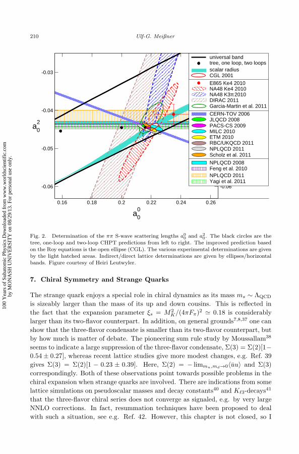
precise verification by a decade. See also Fig. 2 for the present situation for the
comparison of theory and experiment.
And how about lattice QCD, that in principle allows for ab initio calculations
in QCD? First, there are two different paths that allow one to calculate the S-wave
scattering lengths. The first and more direct one is to calculate the low-energy
phase shifts using Luscher’s finite volume approach that relates the energy shift of
an interacting two-particle system in a finite volume to the continuum phase shift.36
This is feasible for the isospin-two scattering length as due to the maximal isospin
in the two-pion system only so-called stretched diagrams contribute, and these
are necessarily connected (that is all valence quark lines run through the whole
Feynman graph). The situation is different for the isospin zero state, that features
also disconnected graphs (where some valence fermion lines are closed and connected
through gluon exchanges to the initial/final state hadrons). Disconnected diagrams
are very noisy in Monte Carlo simulations and thus very hard to compute with
small uncertainties. Therefore, direct computations exist at present only for a20—
and these agree quite well with the prediction (see the horizontal bands in Fig. 2).
The second and indirect method is to compute the LECs ¯3,¯4 (that parametrize
symmetry breaking beyond leading order) and inject these into the pertinent one-
loop formulas for the scattering lengths — this leads to the filled ellipses in Fig. 2
and the agreement with the chiral plus Roy equation prediction is quite good. Still,
the lattice practitioners have to perform the direct computation of a00before they
can claim success — something one has to remind them on a regular basis.
100
Yea
rs o
f Su
bato
mic
Phy
sics
Dow
nloa
ded
from
ww
w.w
orld
scie
ntif
ic.c
omby
MO
NA
SH U
NIV
ER
SIT
Y o
n 08
/29/
13. F
or p
erso
nal u
se o
nly.
May 9, 2013 10:7 World Scientific Review Volume - 9.75in x 6.5in chiral
210 Ulf-G. Meißner
0.16 0.18 0.2 0.22 0.24 0.26
a00
-0.06 -0.06
-0.05 -0.05
-0.04 -0.04
-0.03 -0.03
a20
universal bandtree, one loop, two loopsscalar radius CGL 2001
E865 Ke4 2010NA48 Ke4 2010NA48 K3π 2010DIRAC 2011Garcia-Martin et al. 2011
CERN-TOV 2006JLQCD 2008PACS-CS 2009MILC 2010ETM 2010RBC/UKQCD 2011NPLQCD 2011Scholz et al. 2011
NPLQCD 2008 Feng et al. 2010NPLQCD 2011Yagi et al. 2011
Fig. 2. Determination of the ππ S-wave scattering lengths a00and a2
0. The black circles are the
tree, one-loop and two-loop CHPT predictions from left to right. The improved prediction based
on the Roy equations is the open ellipse (CGL). The various experimental determinations are given
by the light hatched areas. Indirect/direct lattice determinations are given by ellipses/horizontal
bands. Figure courtesy of Heiri Leutwyler.
7. Chiral Symmetry and Strange Quarks
The strange quark enjoys a special role in chiral dynamics as its mass ms ∼ ΛQCD
is sizeably larger than the mass of its up and down cousins. This is reflected in
the fact that the expansion parameter ξs = M2
K/(4πFπ)2' 0.18 is considerably
larger than its two-flavor counterpart. In addition, on general grounds7,8,37 one can
show that the three-flavor condensate is smaller than its two-flavor counterpart, but
by how much is matter of debate. The pioneering sum rule study by Moussallam38
seems to indicate a large suppression of the three-flavor condensate, Σ(3) = Σ(2)[1−
0.54± 0.27], whereas recent lattice studies give more modest changes, e.g. Ref. 39
gives Σ(3) = Σ(2)[1 − 0.23 ± 0.39]. Here, Σ(2) = − limmu,md→0〈uu〉 and Σ(3)
correspondingly. Both of these observations point towards possible problems in the
chiral expansion when strange quarks are involved. There are indications from some
lattice simulations on pseudoscalar masses and decay constants40 and K`3-decays41
that the three-flavor chiral series does not converge as signaled, e.g. by very large
NNLO corrections. In fact, resummation techniques have been proposed to deal
with such a situation, see e.g. Ref. 42. However, this chapter is not closed, so I
100
Yea
rs o
f Su
bato
mic
Phy
sics
Dow
nloa
ded
from
ww
w.w
orld
scie
ntif
ic.c
omby
MO
NA
SH U
NIV
ER
SIT
Y o
n 08
/29/
13. F
or p
erso
nal u
se o
nly.
May 9, 2013 10:7 World Scientific Review Volume - 9.75in x 6.5in chiral
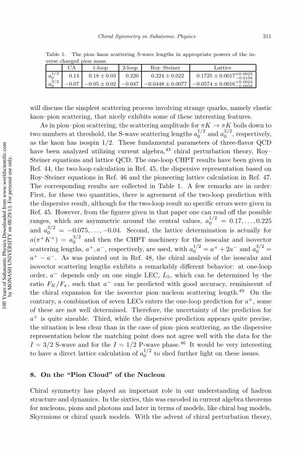
Chiral Symmetry in Subatomic Physics 211
Table 1. The pion–kaon scattering S-wave lengths in appropriate powers of the in-
verse charged pion mass.
CA 1-loop 2-loop Roy–Steiner Lattice
a1/2
00.14 0.18 ± 0.03 0.220 0.224 ± 0.022 0.1725 ± 0.0017+0.0023
−0.0156
a3/20
−0.07 −0.05 ± 0.02 −0.047 −0.0448 ± 0.0077 −0.0574± 0.0016+0.0024−0.0058
will discuss the simplest scattering process involving strange quarks, namely elastic
kaon–pion scattering, that nicely exhibits some of these interesting features.
As in pion–pion scattering, the scattering amplitude for πK → πK boils down to
two numbers at threshold, the S-wave scattering lengths a1/20
and a3/20
, respectively,
as the kaon has isospin 1/2. These fundamental parameters of three-flavor QCD
have been analyzed utilizing current algebra,43 chiral perturbation theory, Roy–
Steiner equations and lattice QCD. The one-loop CHPT results have been given in
Ref. 44, the two-loop calculation in Ref. 45, the dispersive representation based on
Roy–Steiner equations in Ref. 46 and the pioneering lattice calculation in Ref. 47.
The corresponding results are collected in Table 1. A few remarks are in order:
First, for these two quantities, there is agreement of the two-loop prediction with
the dispersive result, although for the two-loop result no specific errors were given in
Ref. 45. However, from the figures given in that paper one can read off the possible
ranges, which are asymmetric around the central values, a1/20
= 0.17, . . . , 0.225
and a3/20
= −0.075, . . . ,−0.04. Second, the lattice determination is actually for
a(π+K+) = a3/20
and then the CHPT machinery for the isoscalar and isovector
scattering lengths, a+, a−, respectively, are used, with a1/20
= a+ + 2a− and a3/20
=
a+ − a−. As was pointed out in Ref. 48, the chiral analysis of the isoscalar and
isovector scattering lengths exhibits a remarkably different behavior: at one-loop
order, a− depends only on one single LEC, L5, which can be determined by the
ratio FK/Fπ, such that a− can be predicted with good accuracy, reminiscent of
the chiral expansion for the isovector pion–nucleon scattering length.49 On the
contrary, a combination of seven LECs enters the one-loop prediction for a+, some
of these are not well determined. Therefore, the uncertainty of the prediction for
a+ is quite sizeable. Third, while the dispersive prediction appears quite precise,
the situation is less clear than in the case of pion–pion scattering, as the dispersive
representation below the matching point does not agree well with the data for the
I = 3/2 S-wave and for the I = 1/2 P-wave phase.46 It would be very interesting
to have a direct lattice calculation of a1/20
to shed further light on these issues.
8. On the “Pion Cloud” of the Nucleon
Chiral symmetry has played an important role in our understanding of hadron
structure and dynamics. In the sixties, this was encoded in current algebra theorems
for nucleons, pions and photons and later in terms of models, like chiral bag models,
Skyrmions or chiral quark models. With the advent of chiral perturbation theory,
100
Yea
rs o
f Su
bato
mic
Phy
sics
Dow
nloa
ded
from
ww
w.w
orld
scie
ntif
ic.c
omby
MO
NA
SH U
NIV
ER
SIT
Y o
n 08
/29/
13. F
or p
erso
nal u
se o
nly.

May 9, 2013 10:7 World Scientific Review Volume - 9.75in x 6.5in chiral
212 Ulf-G. Meißner
it became evident that better founded predictions could be made and with the
ever increasing experimental possibilities, one was finally able to test many of these
predictions. Recent reviews on these exciting developments are Refs. 50 and 51.
Here, I will rather dwell on one particular topic, namely on the so-called “pion
cloud” of the nucleon. This is a much debated topic and regularly leads to heated
discussions — so let us start with a solid definition and then discuss a very recent
application, namely the proton radius puzzle.
Many models of the nucleon feature a compact core (including possibly quarks)
and a longer-ranged component, often called the pion cloud. When I was a graduate
student in the early 1980s, there were heated debates about the size of the inner
core — little bags versus cloudy bags. While one has realized that such debates
were essentially senseless, such type of picture for the nucleon structure remained
(at various levels of sophistication). Clearly, chiral symmetry requires the pion
coupling to the nucleon! In the framework of chiral perturbation theory (in its
pre-EFT formulation) it was realized early that the long-ranged pion cloud can
have profound effects on the structure of the nucleon, i.e. pion loops can lead to
contributions that diverge as 1/Mπ or lnMπ as the pion mass vanishes.52 Such
a behavior is easy to understand, the contributions of massive pions are Yukawa-
suppressed ∼ exp(−Mπr)/r. This suppression becomes Coulomb-like ∼ 1/r (alas of
infinite range) asMπ → 0 and thus divergent matrix elements can emerge. At finite
pion mass, these loop effects contribute with different strength to various nucleon
properties, but they are certainly the best representation of the pion cloud. In
fact, the first calculation of a pion cloud effect dates back to Frazer and Fulco22
long before current algebra — unitarity and analyticity do encode aspects of chiral
symmetry. I will come back to this pioneering calculation later.
As already stated, beyond lowest order, any observable calculated in CHPT re-
ceives contributions from tree and loop graphs. Naively, these loop diagrams qualify
as the natural candidate for a precise definition of the “pion cloud” of any given
hadron. The loop graphs not only generate the imaginary parts of the pertinent
observables but are also — in most cases — divergent, requiring regularization
and renormalization. The method of choice in CHPT is dimensional regularization
(DR), which introduces the scale λ. Varying this scale has no influence on any
observable O (renormalization group invariance),
d
dλO(λ) = 0 , (24)
but this also means that it makes little sense to assign a physical meaning to the sep-
arate contributions from the contact terms and the loops. Physics, however, dictates
the range of scales appropriate for the process under consideration — describing the
pion vector radius (at one loop) by chiral loops alone would necessitate a scale of
about 1/2 TeV (as stressed long ago by Leutwyler). In this case, the coupling of
the ρ-meson generates the strength of the corresponding one-loop counterterm that
gives most of the pion radius. In DR, all one-loop divergences are simple poles
100
Yea
rs o
f Su
bato
mic
Phy
sics
Dow
nloa
ded
from
ww
w.w
orld
scie
ntif
ic.c
omby
MO
NA
SH U
NIV
ER
SIT
Y o
n 08
/29/
13. F
or p
erso
nal u
se o
nly.
May 9, 2013 10:7 World Scientific Review Volume - 9.75in x 6.5in chiral
Chiral Symmetry in Subatomic Physics 213
in 1/(d− 4), where d is the number of space-time dimensions. Consequently, these
divergences can be absorbed in the pertinent LECs that accompany the correspond-
ing local operators at that order in harmony with the underlying symmetries. For a
given LEC, Li this amounts to Li → Lren
i + βi L(λ), where L ∼ 1/(d− 4) and βi is
the corresponding β-function. The renormalized and finite Lren
i must be determined
by a fit to data (or calculated eventually using lattice QCD). Having determined
the values of the LECs from experiment, one is faced with the issue of trying to
understand these numbers. Not surprisingly, the higher mass states of QCD leave
their imprint in the LECs. Consider again the ρ-meson contribution to the vector
radius of the pion. Expanding the ρ-propagator in powers of t/M2
ρ , its first term is
a contact term of dimension four, with the corresponding finite LEC L9 given by
L9 = F 2
π/2M2
ρ ' 7.2 · 10−3, close to the empirical value L9 = 6.9 · 10−3 at λ =Mρ.
This so-called resonance saturation (pioneered in Refs. 53 and 54) holds more gen-
erally for most LECs at one loop and is frequently used in two-loop calculations
to estimate the O(p6) LECs. Let us now discuss the “pion cloud” of the nucleon
in the context of these considerations. Consider as an example the isovector Dirac
radius of the proton.55 The first loop contributions appear at third order in the
chiral expansion, leading to
〈r2〉V1=
(
0.61−(
0.47GeV2)
d(λ) + 0.47 logλ
1GeV
)
fm2, (25)
where d(λ) is a dimension three pion–nucleon LEC that parametrizes the “nucleon
core” contribution. Compared to the empirical value (rv1)2 = 0.585 fm2, we note
that several combinations of (λ, d(λ)) pairs can reproduce the empirical result, e.g.(
1 GeV,+0.06 GeV−2)
,(
0.943 GeV, 0.00 GeV−2)
,(
0.6 GeV,−0.46 GeV−2)
. (26)
An important observation to make is that even the sign of the “core” contribution
to the radius can change within a reasonable range typically used for the scale
λ. Physical intuition would tell us that the value for the coupling d should be
negative such that the nucleon core gives a positive contribution to the isovector
Dirac radius, but field theory tells us that for (quite reasonable) regularization
scales above λ = 943 MeV this need not be the case. In essence, only the sum of
the core and the cloud contribution constitutes a meaningful quantity that should
be discussed. This observation holds for any observable — not just for the isovector
Dirac radius discussed here.
Coming back to the seminal work of Frazer and Fulco — phrased in a more
modern language — they were reconstructing the isovector spectral function of the
nucleon form factors as a product of the pion vector form factor FVπ (t) and the
t-channel P-wave πN partial waves f1
±(t) as (more precisely, we give the results for
the imaginary parts of the Sachs form factors GE and GM , respectively)
Im GVE(t) =
q3
t
mN
√
t(FV
π )∗(t) · f1
+(t) , Im G
VM (t) =
q3
t√
2t(FV
π )∗(t) · f1
−(t) , (27)
100
Yea
rs o
f Su
bato
mic
Phy
sics
Dow
nloa
ded
from
ww
w.w
orld
scie
ntif
ic.c
omby
MO
NA
SH U
NIV
ER
SIT
Y o
n 08
/29/
13. F
or p
erso
nal u
se o
nly.

May 9, 2013 10:7 World Scientific Review Volume - 9.75in x 6.5in chiral
214 Ulf-G. Meißner
0 20 40t [Mπ
2]
0
0.02
0.04
0.06
spec
tral
func
tion
[1/M
π4 ]2ImGE/t
2
2ImGM/t2
Fig. 3. The two-pion spectral function based on modern data for the pion vector form factor.56
The spectral functions weighted by 1/t2 are shown for GE (solid line) and GM (dash-dotted line).
The previous results by Hohler et al.57 (without ρ-ω mixing) are shown for comparison by the
gray/green lines. The dot-dot-dashed (red) line indicates the ρ-meson contribution to Im GM with
a width Γρ = 150MeV.
with qt =√
t/4−M2π the pion momentum in the intermediate state. This repre-
sentation is exact up to t ' 50M2
π. The resulting spectral functions are exhibited
in Fig. 3. The contribution from the ρ-meson is shown by the red dot-dot-dashed
line — the aforementioned enhancement of the two-pion continuum on the left shoul-
der of the resonance is clearly visible. Upon integration, this contribution amounts
to about 50% of the isovector nucleon size, first stressed by Hohler and Pietarinen.58
Naturally, in the one-loop approximation, this mechanism is correctly recovered in
chiral perturbation theory, see e.g. Ref. 59 for a detailed discussion (there, it is
also shown that a similar effect does not appear in the isoscalar spectral functions).
It is remarkable that this so important and visible effect is often ignored in mod-
ern attempts to extract the nucleon size from electron–proton scattering data. This
brings me to the so-called “proton size puzzle.” Until 2010, the electric radius of the
proton was believed to be 0.8768(69) fm (CODATA value),60 from here on referred
to as the “large value”. I would like to stress, however, that the most sophisticated
dispersion theoretical analysis of the nucleon electromagnetic form factors, that in-
clude the two-pion continuum, always led to a small value, rpE ' 0.84 fm.61 In 2010,
the result of the Lamb shift measurement in muonic hydrogen, that are sensitive
to the proton radius, became available: rpE = 0.84184(67) fm.62 This “small value”
led to a flurry of papers questioning either the analysis of the experiment or our
understanding of the proton structure. The underlying theory of strong interac-
tions effects in muonic hydrogen was also scrutinized, see e.g. Refs. 63 and 64.
100
Yea
rs o
f Su
bato
mic
Phy
sics
Dow
nloa
ded
from
ww
w.w
orld
scie
ntif
ic.c
omby
MO
NA
SH U
NIV
ER
SIT
Y o
n 08
/29/
13. F
or p
erso
nal u
se o
nly.

May 9, 2013 10:7 World Scientific Review Volume - 9.75in x 6.5in chiral
Chiral Symmetry in Subatomic Physics 215
The situation was further complicated by the high-precision measurement of
electron–proton scattering at the Mainz Microtron MAMI-C.65 The analysis of these
data led to rpE = 0.879(5)(stat.)(4)(syst.)(2)(model)(4)(group) fm, where the various
types of fits functions (polynomials and splines that do not represent the two-pion
continuum) were used, and depending on the class of fits functions, a model error
is defined and in the end, the results of the two groups of fit functions were av-
eraged, leading to the uncertainty labeled “group”. The Mainz value is in perfect
agreement with the CODATA one but differs by many standard deviations from the
muonic hydrogen result. We have recently reanalyzed the Mainz cross-section data
together with the world data on the neutron form factors. The spectral functions
of the underlying form factors contain besides isoscalar and isovector vector meson
poles the two-pion continuum (updated with new pion form factor data) as well as
representations of the KK66 and the πρ67 continua. For the proton electric and
magnetic radius we find68
rpE = 0.84+0.01
−0.01 fm , rpM = 0.86+0.02
−0.03 fm , (28)
where the uncertainties mostly stem from generous variations of the two-meson
continua. The proton charge radius is completely in agreement with muonic hy-
drogen result — which is entirely due to the inclusion of the two-pion contin-
uum. The magnetic radius is also consistent with earlier determinations, see
e.g. Ref. 69, but again in stark contrast to the analysis of the Mainz group,
rpM = 0.777(13)(stat.)(9)(syst.)(5)(model)(2)(group) fm.65
9. Three-Flavor Chiral Dynamics Reloaded
In the case of three-flavor chiral dynamics with baryons, it was realized early that
the fairly large expansion parameter MK/(4πFπ) ' 0.43 can lead to convergence
problems, see e.g. the pioneering work in Ref. 70. In addition, if one investi-
gates the most fundamental process involving strange quarks and baryons, namely
(anti)kaon–nucleon scattering, the situation is further complicated by the appear-
ance of subthreshold resonances in some channels. More precisely, we have to deal
with the famous Λ(1405) resonance in the isospin zero antikaon-proton interac-
tion, first investigated by Dalitz and Tuan.71 Such a resonance is, of course, not
amenable to a perturbative treatment. However, it was realized by the Munich
group72 that combining chiral symmetry with coupled-channel dynamics allows for
a dynamic generation of such a state (other groups have picked up this idea, see
e.g. Refs. 73–75). To be specific, one considers a Bethe–Salpeter (or Lippman–
Schwinger) equation for the scattering matrix (in a highly symbolic notation),
T = V + V GT , (29)
where V is the potential and G the meson–baryon propagator in the intermediate
state. Here, I have suppressed all channel-indices, so in fact T , V and G are matrices
in channel space. To leading order in the chiral expansion, the potential is given by
100
Yea
rs o
f Su
bato
mic
Phy
sics
Dow
nloa
ded
from
ww
w.w
orld
scie
ntif
ic.c
omby
MO
NA
SH U
NIV
ER
SIT
Y o
n 08
/29/
13. F
or p
erso
nal u
se o
nly.

May 9, 2013 10:7 World Scientific Review Volume - 9.75in x 6.5in chiral
216 Ulf-G. Meißner
the Weinberg-Tomozawa term and the s- and u-channel Born terms. However, the
meson–baryon loop function is divergent and requires regularization. In the early
days, a momentum cutoff was used, but that requires extreme fine-tuning and leads
to a large sensitivity of the results on the choice of the cutoff value. A better method
was proposed in Ref. 74, which is based on a dispersive representation of the loop
function using dimensional regularization with a subtraction constant taking the
role of the regulator. Then, the dependence on the regulator is only logarithmic.
Also, as the power counting is only performed on the level of the potential and
not the scattering matrix, it is absolutely mandatory to calculate the higher order
corrections in V and check a posteriori the convergence in T . Fortunately, this has
been done forK−p scattering,76–78 for S-wave pion–nucleon scattering79 and also for
photo-kaon processes.80 Simply performing calculations with the lowest order chiral
potential is meaningless! Also, in most calculations the on-shell approximation is
used, which turns the integral equations (29) into a set of algebraic equations, that
can be solved easily. However, it is not known how good this approximation really
is, although it seems to work quite well in many cases, see e.g. the early review
Ref. 81. Therefore, calculations avoiding this approximation are required. These are
technically demanding and presently do not incorporate proper crossing symmetry,
for some attempts see Refs. 82–84 and 79. More work in this direction is certainly
required.
Let me now consider the extraction of the (anti)kaon–nucleon scattering lengths.
The one-loop CHPT calculation has been performed by Kaiser.85 It shows that
CHPT converges quite well in the channels without resonances, e.g. for the KN
scattering length with isospin one, quite in contrast to the isospin zero channel,
that features the Λ(1405). There, coupled channel unitarization is required. The
antikaon–nucleon scattering lengths can be extracted from scattering data and also
from the level shift and width of kaonic hydrogen. There has been a long-standing
puzzle related to the discrepancy between the DEAR86 and the earlier and less
accurate KpX experiment at KEK.87 The DEAR data have been puzzling the com-
munity for a long time. As first pointed out in Ref. 88, the energy shift and width
of kaonic hydrogen measured by DEAR is incompatible with the predicted val-
ues taking the underlying KN scattering lengths from scattering data only. This
was resolved by the recent measurement of the energy level shift (ε1s) and width
(Γ1s) of the kaonic hydrogen ground-state by the SIDDHARTA collaboration,89
ε1s = −283±36 (stat)±6 (syst) eV , and Γ1s = 541±89 (stat)±22 (syst) eV. Two
groups have taken up the charge and shown that the SIDDHARTA data together
with the older scattering data indeed allow for a fairly precise determination of the
K−p scattering lengths, based on the chiral potential at NLO.90,91 I collect here the
results obtained in Ref. 91, noting that they are quite consistent with the earlier
results of Ref. 90. The values for the K−p scattering lengths are
a0 = −1.81+0.30−0.28 + i 0.92+0.29
−0.23 fm , a1 = +0.48+0.12−0.11 + i 0.87+0.26
−0.20 fm . (30)
100
Yea
rs o
f Su
bato
mic
Phy
sics
Dow
nloa
ded
from
ww
w.w
orld
scie
ntif
ic.c
omby
MO
NA
SH U
NIV
ER
SIT
Y o
n 08
/29/
13. F
or p
erso
nal u
se o
nly.
May 9, 2013 10:7 World Scientific Review Volume - 9.75in x 6.5in chiral
Chiral Symmetry in Subatomic Physics 217
óóçç
ææ
ó ó
´
çç
ææ
-2 -1 0 10.2
0.4
0.6
0.8
1.0
1.2
1.4
Re a@fmD
Ima@
fmD
a0
a1
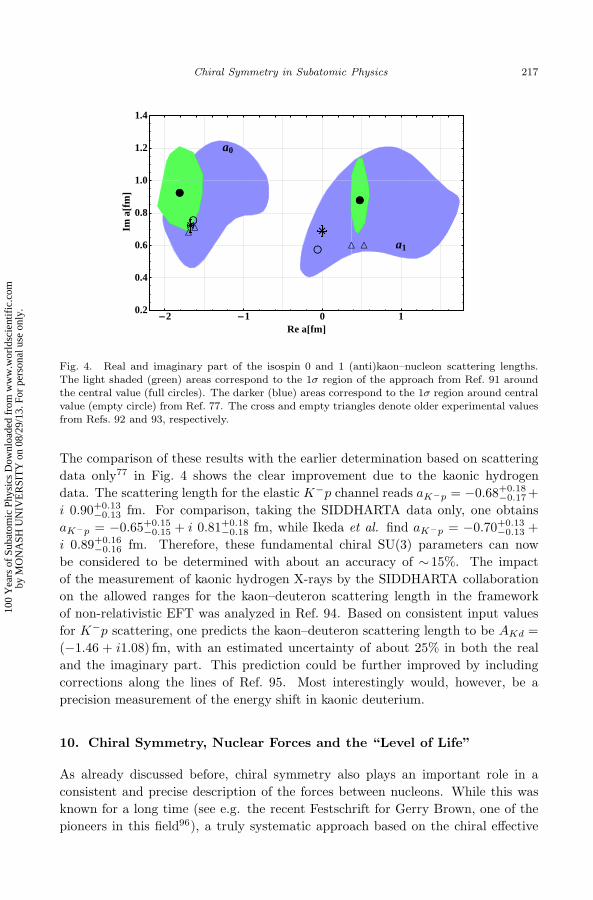
Fig. 4. Real and imaginary part of the isospin 0 and 1 (anti)kaon–nucleon scattering lengths.
The light shaded (green) areas correspond to the 1σ region of the approach from Ref. 91 around
the central value (full circles). The darker (blue) areas correspond to the 1σ region around central
value (empty circle) from Ref. 77. The cross and empty triangles denote older experimental values
from Refs. 92 and 93, respectively.
The comparison of these results with the earlier determination based on scattering
data only77 in Fig. 4 shows the clear improvement due to the kaonic hydrogen
data. The scattering length for the elastic K−p channel reads aK−p = −0.68+0.18−0.17+
i 0.90+0.13−0.13 fm. For comparison, taking the SIDDHARTA data only, one obtains
aK−p = −0.65+0.15−0.15 + i 0.81+0.18
−0.18 fm, while Ikeda et al. find aK−p = −0.70+0.13−0.13 +
i 0.89+0.16−0.16 fm. Therefore, these fundamental chiral SU(3) parameters can now
be considered to be determined with about an accuracy of ∼ 15%. The impact
of the measurement of kaonic hydrogen X-rays by the SIDDHARTA collaboration
on the allowed ranges for the kaon–deuteron scattering length in the framework
of non-relativistic EFT was analyzed in Ref. 94. Based on consistent input values
for K−p scattering, one predicts the kaon–deuteron scattering length to be AKd =
(−1.46 + i1.08) fm, with an estimated uncertainty of about 25% in both the real
and the imaginary part. This prediction could be further improved by including
corrections along the lines of Ref. 95. Most interestingly would, however, be a
precision measurement of the energy shift in kaonic deuterium.
10. Chiral Symmetry, Nuclear Forces and the “Level of Life”
As already discussed before, chiral symmetry also plays an important role in a
consistent and precise description of the forces between nucleons. While this was
known for a long time (see e.g. the recent Festschrift for Gerry Brown, one of the
pioneers in this field96), a truly systematic approach based on the chiral effective
100
Yea
rs o
f Su
bato
mic
Phy
sics
Dow
nloa
ded
from
ww
w.w
orld
scie
ntif
ic.c
omby
MO
NA
SH U
NIV
ER
SIT
Y o
n 08
/29/
13. F
or p
erso
nal u
se o
nly.
May 9, 2013 10:7 World Scientific Review Volume - 9.75in x 6.5in chiral
218 Ulf-G. Meißner
Lagrangian of QCD only became available through the groundbreaking work of
Weinberg.97 As realized by Weinberg, the power counting does not apply directly to
the S-matrix, but rather to the effective potential — these are all diagrams without
N -nucleon intermediate states. Such diagrams lead to pinch singularities in the
infinite nucleon mass limit (the so-called static limit), so that, e.g. the nucleon box
graph is enhanced as m/Q2, with m the nucleon mass and Q a small momentum.
The power counting formula for the graphs contributing with the νth power of Q
or a pion mass to the effective potential reads (considering only connected pieces):
ν = 2−N − 2L+∑
i
Vi
[
di +ni
2− 2
]
. (31)
Here, N is the number of in-coming and out-going nucleons, L the number of pion
loops, Vi counts the vertices of type i with di derivatives and/or pion mass insertions
and ni is the number of nucleons participating in this kind of vertex. Because of
chiral symmetry, the term in the square brackets is larger than or equal to zero and
thus the leading terms contributing, e.g., to the two-nucleon potential can easily
be identified. These are the time-honored one-pion exchange and two four-nucleon
contact interactions without derivatives. The so-constructed effective potential is
then iterated in the Schrodinger or Lippman–Schwinger equation, generating the
shallow nuclear bound states as well as scattering states. The resulting contribu-
tions at various orders to the 2N , the 3N and the 4N forces are depicted in Fig. 5.
Remarkably, by now the 2N , 3N and 4N force contributions have been worked out
to NNNLO, the last missing piece, namely the short-range and 1/mN -corrections
to the 3N forces, was only provided recently.98 This EFT approach shares a few
advantages over the very well developed and precise semi-phenomenological ap-
proaches, just to mention the consistent derivation of 2N , 3N and 4N forces as
well as electroweak current operators, the possibility to work out theoretical uncer-
tainties and to improve the precision by going to higher orders and, of course, the
direct connection to the spontaneously and explicitely broken chiral symmetry of
QCD. There has been a large body of work on testing and developing these forces
in few-nucleon systems, for comprehensive reviews see Refs. 99 and 100.
As one beautiful example of combining chiral perturbation theory calculations
and nuclear EFT, I want to discuss the recent extraction of the fundamental S-wave
pion–nucleon scattering lengths from the high-precision data on pionic hydrogen and
deuterium taken at PSI.101,102 To achieve the corresponding precision in theory, the
authors of Ref. 103 used chiral perturbation theory to calculate the π−d scattering
length with an accuracy of a few percent, including isospin-violating corrections both
in the two- and three-body sector. Here, two- and three-body refers to the photon
coupling to the two-nucleon and the two-nucleon plus one pion intermediate states,
in more conventional language the impulse approximation and the meson-exchange
current contributions, respectively. In particular, the isospin-breaking contributions
to the three-body part of aπ−d due to mass differences, isospin violation in the πN
scattering lengths, and virtual photons were studied. This last class of effects is
100
Yea
rs o
f Su
bato
mic
Phy
sics
Dow
nloa
ded
from
ww
w.w
orld
scie
ntif
ic.c
omby
MO
NA
SH U
NIV
ER
SIT
Y o
n 08
/29/
13. F
or p
erso
nal u
se o
nly.

May 9, 2013 10:7 World Scientific Review Volume - 9.75in x 6.5in chiral
Chiral Symmetry in Subatomic Physics 219
2N LO
N LO3
NLO
LO
3N force 4N force2N force
Fig. 5. Contributions to the effective potential of the 2N , 3N and 4N forces based on Weinberg’s
power counting. Here, LO denotes leading order, NLO next-to-leading order and so on. Dimension
one, two and three pion–nucleon interactions are denoted by small circles, big circles and filled
boxes, respectively. In the 4N contact terms, the filled and open box denote two- and four-
derivative operators, respectively.
ostensibly infrared enhanced due to the smallness of the deuteron binding energy.
However, the authors of Ref. 103 showed that the leading virtual-photon effects that
might undergo such enhancement cancel, and hence the standard chiral perturbation
theory (Weinberg) counting provides a reliable estimate of isospin violation in aπ−d
due to virtual photons. This allowed to extract the isoscalar and isovector scattering
lengths to high precision, see also Fig. 6,
a+ = (7.6± 3.1) · 10−3
/Mπ , a− = (86.1± 0.9) · 10−3
/Mπ . (32)
Most remarkable is the fact that for the first time, the small isoscalar scatter-
ing length could be extracted with a definite sign, this was not possible based
on scattering data only, see e.g. Ref. 104. Also, one should note that the dom-
inant isovector scattering length could be determined with an uncertainty of 1%
only — this is truly amazing and demonstrates again the power of combining
EFT with chiral symmetry. In fact, the LO chiral perturbation theory result
of Weinberg already nicely captures the essence of these results, a+CA
= 0 and
a−CA
= (M2
π/8πF2
π)/(1 +Mπ/mp) = 79.5 · 10−3/Mπ, but only now one knows pre-
cisely how much these are affected by higher order corrections — the first attempt
to calculate these dates back almost two decades.105
Now I turn to the nuclear many-body problem. More precisely, this refers to
nuclei with atomic number A > 4. Nuclear lattice simulations combine the power
100
Yea
rs o
f Su
bato
mic
Phy
sics
Dow
nloa
ded
from
ww
w.w
orld
scie
ntif
ic.c
omby
MO
NA
SH U
NIV
ER
SIT
Y o
n 08
/29/
13. F
or p
erso
nal u
se o
nly.

May 9, 2013 10:7 World Scientific Review Volume - 9.75in x 6.5in chiral
220 Ulf-G. Meißner
xxxxxxxxxxxxxxxxxxxxxxxxxxxxxxxxxxxxxxxxxxxxxxxxxxxxxxxxxxxxxxxxxxxxxxxxxxxxxxxxxxxxxxxxxxxxxxxxxxxxxxxxxxxxxxxxxxxxxxxxxxxxxxxxxxxxxxxxxxxxxxxxxxxxxxxxxxxxxxxxxxxxxxxxxxxxxxxxxxxxxxxxxxxxxxxxxxxxxxxxxxxxxxxxxxxxxxxxxxxxxxxxxxxxxxxxxxxxxxxxxxxxxxxxxxxxxxxxxxxxxxxxxxxxxxxxxxxxxxxxxxxxxxxxxx
xxxxxxxxxxxxxxxxxxxxxxxxxxxxxxxxxxxxxxxxxxxxxxxxxxxxxxxxxxxxxxxxxxxxxxxxxxxxxxxxxxxxxxxxxxxxxxxxxxxxxxxxxxxxxxxxxxxxxxxxxxxxxxxxxxxxxxxxxxxxxxxxxxxxxxxxxxxxxxxxxxxxxxxxxxxxxxxxxxxxxxxxxxxxxxxxxxxxxxxxxxxxxxxxxxxxxxxxxxxxxxxxxxxxxxxxxxxxxxxxxxxxxxxxxxxxxxxxxxxxxxxxxxxxxxxxxxxxxxxxxxxxxxxxxxxxxxxxxxxxxxxxxxxxxxxxxxxxxxxxxxxxxxxxxxxxxxxxxxxxxxxxxxxxxxxxxxxxxxxxxxxxxxxxxxxxxxxxxxxxxxxxxxxxxxxxxxxxxxxxxxxxxxxxxxxxxxxxxxxxxxxxxxxxxxxxxxxxxxxxxxxxxxxxxxxxxxxxxxxxxxxxxxxxxxxxxxxxxxxxxxxxxxxxxxxxxxxxxxxxxxxxxxxxxxxxxxxxxxxxxxxxxxxxxxxxxxxxxxxxxxxxxxxxxxxxxxxxxxxxxxxxxxxxxxxxxxxxxxxxxxxxxxxxxxxxxxxxxxxxxxxxxxxxxxxxxxxxxxxxxxxxxxxxxxxxxxxxxxxxxxxxxxxxxxxxxxxxxxxxxxxxxxxxxxxxxxxxxxxxxxxxxxxxxxxxxxxxxxxxxxxxxxxxxxxxxxxxxxxxxxxxxxxxxxxxxxxxxxxxxxxxxxxxxxxxxxxxxxxxxxxxxxxxxxxxxxxxxxxxxxxxxxxxxxxxxxxxxxxxxxxxxxxxxxxxxxxxxxxxxxxxxxxxxxxxxxxxxxxxxxxxxxxxxxxxxxxxxxxxxxxxxxxxxxxxxxxxxxxxxxxxxxxxxxxxxxxxxxxxxxxxxxxxxxxxxxxxxxxxxxxxxxxxxxxxxxxxxxxxxxxxxxxxxxxxxxxxxxxxxxxxxxxxxxxxxxxxxxxxxxxxxxxxxxxxxxxxxxxxxxxxxxxxxxxxxxxxxxxxxxxxxxxxxxxxxxxxxxxxxxxxxxxxxxxxxxxxxxxxxxxxxxxxxxxxxxxxxxxxxxxxxxxxxxxxxxxxxxxxxxxxxxxxxxxxxxxxxxxx
xxxxxxxxxxxxxxxxxxxxxxxxxxxxxxxxxxxxxxxxxxxxxxxxxxxxxxxxxxxxxxxxxxxxxxxxxxxxxxxxxxxxxxxxxxxxxxxxxxxxxxxxxxxxxxxxxxxxxxxxxxxxxxxxxxxxxxxxxxxxxxxxxxxxxxxxxxxxxxxxxxxxxxxxxxxxxxxxxxxxxxxxxxxxxxxxxxxxxxxxxxxxxxxxxxxxxxxxxxxxxxxxxxxxxxxxxxxxxxxxxxxxxxxxxxxxxxxxxxxxxxxxxxxxxxxxxxxxxxxxxxxxxxxxxxxxxxxxxxxxxxxxxxxxxxxxxxxxxxxxxxxxxxxxxxxxxxxxxxxxxxxxxxxxxxxxxxxxxxxx
xxxxxxxxxxxxxxxxxxxxxxxxxxxx
Fig. 6. Constraints in the a+-a− plane from the data on pionic hydrogen (level shift and width)
and pionic deuterium (level shift). For the precise relation between the quantity a+ and the
scattering length a+, see Ref. 103. Figure courtesy of Martin Hoferichter.
of EFT to generate few-nucleon forces with numerical methods to exactly solve the
non-relativistic A-body system, where in a nucleus A counts the number of neu-
trons plus protons. For a detailed review, I refer to Ref. 106 and here I give only
a very short account of this method. The basic idea is to introduce a smallest
length (the lattice spacing) in the spatial directions and in the temporal direction,
denoted a and at, respectively and then to discretize the finite space-time volume
L × L × L × Lt in integer numbers of a and at. A Wick rotation to Euclidean
space is naturally implied. Note that the lattice spacing entails an UV cutoff (a
maximal momentum), pmax = π/a. In typical simulations of atomic nuclei, one has
a ' 2 fm and thus pmax ' 300MeV. In contrast to lattice QCD, the continuum limit
a → 0 is not taken. This formulation allows to calculate the correlation function
Z(t) = 〈ψA| exp(−tH)|ψA〉, where t is the Euclidean time and |ψA〉 an A–nucleon
state. Using standard methods, one can derive any observable from the correlation
function, e.g. the ground-state energy is simply the infinite time limit of the loga-
rithmic derivative of Z(t) with respect to the time. Similarly, excited states can be
generated by starting with an ensemble of standing waves, generating a correlation
matrix Zji(t) = 〈ψjA| exp(−tH)|ψi
A〉, which upon projection onto internal quantum
numbers and diagonalization generates the ground and excited states — the larger
the initial state basis, the more excited states can be extracted. Another recently
developed method is based on position-space wave functions.107 In a first step, one
constructs from the general wave functions ψj(~n ) (j = 1, . . . , A) states with well-
100
Yea
rs o
f Su
bato
mic
Phy
sics
Dow
nloa
ded
from
ww
w.w
orld
scie
ntif
ic.c
omby
MO
NA
SH U
NIV
ER
SIT
Y o
n 08
/29/
13. F
or p
erso
nal u
se o
nly.

May 9, 2013 10:7 World Scientific Review Volume - 9.75in x 6.5in chiral
Chiral Symmetry in Subatomic Physics 221
Table 2. The even-parity spectrum of 12C from nuclear lattice simulations. The ground state is
denoted as O+
1and the Hoyle state as O+
2. The NLO corrections include strong isospin breaking
as well as the Coulomb force. The NNLO corrections are generated by the leading three-nucleon
forces. The theoretical errors include both Monte Carlo statistical errors and uncertainties due to
extrapolation at large Euclidean time.
0+1
2+1
0+2
2+2
LO −96(2) MeV −94(2) MeV −88(2) MeV −84(2) MeV
NLO −77(3) MeV −72(3) MeV −71(3) MeV −66(3) MeV
NNLO −92(3) MeV −86(3) MeV −84(3) MeV −79(3) MeV
−80.7(4) MeV (Ref. 117)
Exp. −92.2 MeV −87.7 MeV −84.5 MeV −82.6 MeV (Ref. 118)
−81.1(3) MeV (Ref. 119)
defined momentum using all possible translations, L−3/2∑
~m ψj(~n+ ~m ) exp(i ~P · ~m).
A proper choice for the ψj allows one to prepare certain types of initial states, such
as shell-model wave functions,
ψj(~n ) = exp[−c~n2] , ψ′j(~n ) = nx exp[−c~n
2] , ψ′′j (~n ) = ny exp[−c~n
2] , . . . , (33)
or, for later use, alpha-cluster wave functions,
ψj(~n ) = exp[−c(~n− ~m)2] , ψ′j(~n ) = exp[−c(~n− ~m
′)2] , . . . . (34)
The possibility to construct all these different types of initial/final states is a reflec-
tion of the fact that in the underlying EFT all possible configurations to distribute
nucleons over all lattice sites are generated. This includes in particular the con-
figuration where four nucleons are located at one space-time point, so there is no
restriction like, e.g. in a no-core-shell model approach, in which one encounters se-
rious problems with the phenomenon of clustering, that is so prominent in nuclear
physics. It is also important to note that the nuclear forces have an approximate
spin–isospin SU(4) symmetry (Wigner symmetry)108 that is of fundamental impor-
tance in suppressing the malicious sign oscillations that plague any Monte Carlo
simulation of strongly interacting fermion systems at finite density. The relation
of the Wigner symmetry to the nuclear EFT formulation has been worked out in
Ref. 109.
As one application of this method, I want to discuss the so-called Hoyle state.
It plays a crucial role in the helium burning of stars heavier than our sun and in
the production of carbon and other elements necessary for life. This excited state
of 12C was postulated by Hoyle110 as a necessary ingredient for the fusion of three
α-particles to produce a sufficient amount of carbon at stellar temperatures. For
this reason, the Hoyle state plays also a very important role in the context of the
anthropic principle, although such considerations did not play any role when this
state was predicted.111 The Hoyle state was dubbed the “level of life” by Andrei
Linde.112 This excited state has been an enigma for nuclear structure theory since
decades, even the most successful Greens function MC methods based on realis-
tic two- and three-nucleon forces113 or the no-core-shell-model employing modern
(chiral or Vlow k) interactions114,115 have not been able to describe this state. The
100
Yea
rs o
f Su
bato
mic
Phy
sics
Dow
nloa
ded
from
ww
w.w
orld
scie
ntif
ic.c
omby
MO
NA
SH U
NIV
ER
SIT
Y o
n 08
/29/
13. F
or p
erso
nal u
se o
nly.
May 9, 2013 10:7 World Scientific Review Volume - 9.75in x 6.5in chiral
222 Ulf-G. Meißner
first ab initio calculation of the Hoyle state based on nuclear lattice simulations was
reported in Ref. 116. In the meantime, the calculation of the spectrum of 12C has
been considerably improved, using the aforementioned position-space initial and
final state wave functions. The predictions for the even-parity states in the 12C
spectrum are collected in Table 2. In all cases, the LO calculation is within 10%
of the experimental number, and the three-nucleon forces at NNLO are essential to
achieve agreement with experiment. The Hoyle state is clearly recovered and comes
out at almost the same energy as the 4He + 8Be threshold — thus allowing for
the resonant enhancement of carbon production that was first considered by Hoyle
half a century ago. Furthermore, one finds a second 2+ excited state that has been
much debated in the literature. Recent determinations of this level based on various
methods (alpha and proton scattering off 12C as well as an R-matrix analysis of the
β-decays of 12N and 12B) are in fair agreement with the calculation. The chiral
nuclear EFT will also allow one to investigate how the closeness of the Hoyle state
to the 4He + 8Be threshold depends on the fundamental parameters like the light
quark masses, thus allowing for a test of the anthropic principle. For a first attempt
within a alpha-cluster model, see Ref. 120.
11. Chiral Symmetry and Heavy Quarks
Naively, chiral symmetry has little to do with the physics of heavy quarks as the
sectors of light and heavy quarks are quite different in QCD. However, it was realized
in the early 1990s that chiral and heavy quark symmetry can indeed be intertwined
in decays and reactions of heavy hadrons. The implications of chiral symmetry
for heavy hadron physics was pioneered by Wise,121 Burdman and Donoghue122
and the group of Yan et al.123 This field has become ever more important since
then partly due to the many puzzling results that have emerged in charm quark
spectroscopy. The phenomenology of heavy meson chiral Lagrangians has been
reviewed in Ref. 124.
Arguably, the most interesting interplay between chiral and heavy quark dy-
namics are the decays of ψ′ into J/ψπ0 and J/ψη that were suggested to be a
reliable source for extracting the light quark mass ratio mu/md.125,126 See also the
review by Donoghue on “Light quark masses and chiral symmetry.”127 The decay
ψ′→ J/ψπ0 violates isospin symmetry. Both the up-down quark mass difference
and the electromagnetic (em) interaction can contribute to isospin breaking. How-
ever, it was shown that the em contribution to the decay ψ′→ J/ψπ0 is much
smaller than the effect of the quark mass difference.128,129 Based on the QCD mul-
tipole expansion and the axial anomaly, the relation between the quark mass ratio
1/R ≡ (md −mu)/(ms − m), where m = (md +mu)/2, and the ratio of the decay
widths of these two decays was worked out up to the next-to-leading order in the
100
Yea
rs o
f Su
bato
mic
Phy
sics
Dow
nloa
ded
from
ww
w.w
orld
scie
ntif
ic.c
omby
MO
NA
SH U
NIV
ER
SIT
Y o
n 08
/29/
13. F
or p
erso
nal u
se o
nly.
May 9, 2013 10:7 World Scientific Review Volume - 9.75in x 6.5in chiral
Chiral Symmetry in Subatomic Physics 223
chiral expansion.130,131 One obtains
Γ(ψ′→ J/ψπ0)
Γ(ψ′→ J/ψη)
= 3
(
md −mu
md +mu
)2F 2
π
F 2η
M4
π
M4η
∣
∣
∣
∣
~qπ
~qη
∣
∣
∣
∣
3
, (35)
where Fπ(η) and Mπ(η) are the decay constant and mass of the pion (eta), respec-
tively, and ~qπ(η) is the pion (eta) momentum in the ψ′ rest frame. The most recent
measurement of the decay-width ratio,132 Rπ0/η = (3.88±0.23±0.05) allows one in
principle to extract the quark mass ratio R within a few percent precision, see e.g.
Ref. 133 for an earlier use of this approach. However, it was shown in Ref. 134 that
effects due to charmed meson triangle diagrams (dispersive effects) are much larger
than originally thought and that the sizeable uncertainty related to the calculation
of these effects makes a precise extraction of the light quark mass ratio from these
decays very difficult. Quite in contrast to the charmonium system, similar transi-
tions in the bottomnium spectrum that are sensitive to the quark masses are not
afflicted with such large heavy meson loop effects, as explained in detail in Ref. 135.
An intriguing implication of this suppression of the bottom meson loops in the tran-
sitions Υ(4S) → hbπ0(η) is that the decay amplitudes are dominated by the quark
mass differences, and hence it is possible to extract the light quark mass ratio from
the ratio of the branching fractions of the transitions Υ(4S) → hbπ0(η) with good
accuracy. The theoretical uncertainty on the extraction of the light quark mass
ratio mu/md has been estimated in Ref. 135 to be about 25%. Now it remains to
be seen how precisely the decays Υ(4S) → hbπ0 and Υ(4S) → hbη can be measured.
Finally, I only want to discuss a recent application of the interplay of chiral
symmetry, lattice QCD and charmonium physics.136 Charmonium states, the most
prominent one being the J/ψ, are bound states of a heavy quark and a heavy anti-
quark, so in general heavy quarkonia do not contain any valence light quarks. Thus,
one would naively expect that the light quark mass dependence of their properties
would be suppressed, so that one can use a simple formula linear in the light quark
masses to do the chiral extrapolation, as done in, e.g. Refs. 137 and 138 for the
mass splittings. The higher order corrections to the charmonium mass splittings
were already analyzed a long time ago in Ref. 139. While such a lowest order extrap-
olation might be sufficient for the low-lying states, a similar simple extrapolation
may not be reasonable for the higher excited states. In fact, dramatic and even
non-analytic dependences in the light quark masses can arise. Hence, for the ex-
cited states which are close to open-flavor thresholds, a formula taking into account
the non-analyticity should be utilized for the chiral extrapolation. Furthermore, for
the radiative transitions with strong coupled-channel effects, simulations at several
pion masses are necessary in order to extract the physical results. The effects of
light quarks in heavy quarkonium systems are due to quantum fluctuations of the
sea quarks. Sea quark and antiquark pairs are created and annihilated in the color
singlet heavy quarkonium. The low-energy fluctuations can be described in the
framework of chiral perturbation theory. The quarkonium states can be included
100
Yea
rs o
f Su
bato
mic
Phy
sics
Dow
nloa
ded
from
ww
w.w
orld
scie
ntif
ic.c
omby
MO
NA
SH U
NIV
ER
SIT
Y o
n 08
/29/
13. F
or p
erso
nal u
se o
nly.

May 9, 2013 10:7 World Scientific Review Volume - 9.75in x 6.5in chiral
224 Ulf-G. Meißner
as matter fields. Let me focus on the quark mass dependence of the quarkonium
mass. Two types of sea quark fluctuations are possible. Class (a) can be described
by closed light quark loops that are disconnected from the heavy quark–antiquark
systems. Such diagrams are suppressed according to the Okuba–Zweig–Iizuka rule.
Class (b) subsumes all diagrams in which the heavy quark (antiquark) and the vir-
tual sea antiquark (quark) can form a color singlet state, a heavy meson (antime-
son), i.e. a pair of virtual heavy meson and antimeson is created and annihilated
after a short propagation. Type (a) can be parametrized using an effective chiral
Lagrangian containing unknown low-energy constants. The resulting quark mass
dependence is analytic in the light quark masses up to chiral logarithms. Complex-
ity comes from fluctuations of type (b), which can lead to non-analyticity. This is
indeed the case for states that are close to open-flavor thresholds. For such a state,
the appropriate chiral extrapolation formula for its mass M takes the form
M(Mπ) =◦
M + dM2
π +√
e+ fM2π , (36)
where◦
M (the hadron mass in the chiral limit), d, e and f are parameters to be fit
to the lattice data. For states far away from any open-flavor threshold, e will be
much larger than fM2
π so that the square root can be expanded, and one may use
only the first two terms in the above equation up to O(M2
π). Explicit modeling of
various charmonium excitations indeed shows that the light quark mass dependence
is not always suppressed for heavy quarkonium systems.136 As an example, the
decay widths of the hindered M1 transitions between P-wave charmonia (see e.g.
Ref. 140) have a strong dependence on the pion mass. Lattice results at a pion
mass around 500 MeV can deviate by a factor of two from the actual values at the
physical pion mass. It would be interesting to investigate how such effects would
affect the recent lattice results for excited and exotic charmonium spectroscopy that
have been obtained for pion masses of about 400 MeV.141
12. Some Final Remarks
In this contribution, I have elucidated the role of chiral symmetry in hadronic and
nuclear physics, stressing the many connections between various seemingly disjunct
fields. Chiral perturbation theory as the effective field theory of the strong interac-
tions has matured over the years and methods have developed to either sharpen its
predictions or enlarge its range of validity. Also, the strange quark plays a special
role — chiral three-flavor dynamics is only one of the frontiers of research, where a
union of chiral symmetry and lattice simulations will play an even more important
role in the years to come. Furthermore, the fruitful interplay between chiral symme-
try and dispersion relations is expected to shed more light on scattering processes
and resonance excitation. In nuclear physics, three-nucleon forces are presently
at the forefront of structure research, where it is practically unthinkable to make
progress without invoking the powerful constraints from chiral symmetry. I would
100
Yea
rs o
f Su
bato
mic
Phy
sics
Dow
nloa
ded
from
ww
w.w
orld
scie
ntif
ic.c
omby
MO
NA
SH U
NIV
ER
SIT
Y o
n 08
/29/
13. F
or p
erso
nal u
se o
nly.

May 9, 2013 10:7 World Scientific Review Volume - 9.75in x 6.5in chiral
Chiral Symmetry in Subatomic Physics 225
like to finish with one comment. Often it is said that chiral perturbation theory will
not be needed any more as the lattice starts to generate results at physical quark
masses. What a misconception! Time will show that chiral symmetry will continue
to be one major ingredients to understand the physics encoded in all these numbers
that will be generated from lattice QCD simulations in the years to come.
Acknowledgments
I would like to thank Ernest Henley for giving me the opportunity to contribute to
this volume. All my collaborators are thanked for sharing their insights into the
topics discussed here. I thank Veronique Bernard, Feng-Kun Guo and Dean Lee for
a careful reading of this manuscript. This work was supported in part by the DFG
(SFB/TR 16 and SFB/TR 110), the BMBF (grant 06BN9006), the HGF (grant
VH-VI-417) and the EU (FP7, HadronPhysics3).
References
1. S. Weinberg, Physica A 96, 327 (1979).
2. J. Gasser and H. Leutwyler, Annals Phys. 158, 142 (1984).
3. J. Gasser and H. Leutwyler, Nucl. Phys. B 250, 465 (1985).
4. J. Goldstone, Nuovo Cim. 19, 154 (1961).
5. J. Goldstone, A. Salam and S. Weinberg, Phys. Rev. 127, 965 (1962).
6. C. Vafa and E. Witten, Nucl. Phys. B 234, 173 (1984).
7. T. Banks and A. Casher, Nucl. Phys. B 169, 103 (1980).
8. H. Leutwyler and A. Smilga, Phys. Rev. D 46, 5607 (1992).
9. J. Stern, arXiv:hep-ph/9801282.
10. M. Gell-Mann and Y. Ne’eman, The Eightfold Way (W. A. Benjamin, New York,
1964).
11. K. Fujikawa, Phys. Rev. D 29, 285 (1984).
12. J. Bijnens, Int. J. Mod. Phys. A 8, 3045 (1993).
13. G. Colangelo et al., Eur. Phys. J. C 71, 1695 (2011) [arXiv:1011.4408 [hep-lat]].
14. T. R. Hemmert, B. R. Holstein and J. Kambor, J. Phys. G 24, 1831 (1998) [hep-
ph/9712496].
15. P. C. Bruns and U.-G. Meißner, Eur. Phys. J. C 40 (2005) 97 [hep-ph/0411223].
16. S. Leupold and M. F. M. Lutz, Eur. Phys. J. A 39, 205 (2009) [arXiv:0807.4686
[hep-ph]].
17. D. Djukanovic, J. Gegelia, A. Keller and S. Scherer, Phys. Lett. B 680, 235 (2009)
[arXiv:0902.4347 [hep-ph]].
18. H. Leutwyler, Annals Phys. 235, 165(1994) [hep-ph/9311274].
19. E. D’Hoker and S. Weinberg, Phys. Rev. D 50, 6050 (1994) [hep-ph/9409402].
20. V. Bernard, N. Kaiser and U.-G. Meißner, Int. J. Mod. Phys. E 4, 193 (1995) [hep-
ph/9501384].
21. M. C. M. Rentmeester, R. G. E. Timmermans, J. L. Friar and J. J. de Swart, Phys.Rev. Lett. 82, 4992 (1999). [nucl-th/9901054].
22. W. R. Frazer and J. R. Fulco, Phys. Rev. Lett. 2, 365 (1959); Phys. Rev. 117, 1609(1960).
23. H. Lehmann, Phys. Lett. B 41, 529 (1972).
100
Yea
rs o
f Su
bato
mic
Phy
sics
Dow
nloa
ded
from
ww
w.w
orld
scie
ntif
ic.c
omby
MO
NA
SH U
NIV
ER
SIT
Y o
n 08
/29/
13. F
or p
erso
nal u
se o
nly.

May 9, 2013 10:7 World Scientific Review Volume - 9.75in x 6.5in chiral
226 Ulf-G. Meißner
24. V. Bernard and U.-G. Meißner, Ann. Rev. Nucl. Part. Sci. 57, 33 (2007) [hep-
ph/0611231].
25. T. N. Truong, Phys. Rev. Lett. 67, 2260 (1991).
26. J. Gasser, PoS EFT 09, 029 (2009).
27. S. Weinberg, Phys. Rev. Lett. 17, 616 (1966).
28. J. Gasser and H. Leutwyler, Phys. Lett. B 125, 325 (1983).
29. J. Bijnens, G. Colangelo, G. Ecker, J. Gasser and M. E. Sainio, Phys. Lett. B 374,
210 (1996) [hep-ph/9511397].
30. J. F. Donoghue, B. R. Holstein and Y. C. Lin, Phys. Rev. D 37, 2423 (1988).
31. J. Gasser and U.-G. Meißner, Nucl. Phys. B 357, 90 (1991).
32. G. Colangelo, J. Gasser and H. Leutwyler, Phys. Lett. B 488, 261 (2000) [hep-
ph/0007112].
33. G. Colangelo, J. Gasser and A. Rusetsky, Eur. Phys. J. C 59, 777 (2009)
[arXiv:0811.0775 [hep-ph]].
34. J. Gasser, B. Kubis and A. Rusetsky, Nucl. Phys. B 850, 96 (2011) [arXiv:1103.4273
[hep-ph]].
35. J. R. Batley et al. [NA48-2 Collaboration], Eur. Phys. J. C 70, 635 (2010).
36. M. Luscher, Nucl. Phys. B 354, 531 (1991).
37. C. Vafa and E. Witten, Commun. Math. Phys. 95, 257 (1984).
38. B. Moussallam, Eur. Phys. J. C 14, 111 (2000) [hep-ph/9909292].
39. H. Fukaya et al. [JLQCD and TWQCD Collaboration], Phys. Rev. D 83, 074501
(2011) [arXiv:1012.4052 [hep-lat]].
40. C. Allton et al. [RBC-UKQCD Collaboration], Phys. Rev. D 78, 114509 (2008)
[arXiv:0804.0473 [hep-lat]].
41. P. A. Boyle, A. Juttner, R. D. Kenway, C. T. Sachrajda, S. Sasaki, A. Soni,
R. J. Tweedie and J. M. Zanotti, Phys. Rev. Lett. 100, 141601 (2008)
[arXiv:0710.5136 [hep-lat]].
42. V. Bernard, S. Descotes-Genon and G. Toucas, JHEP 1101, 107 (2011)
[arXiv:1009.5066 [hep-ph]].
43. R. W. Griffith, Phys. Rev. 176, 1705 (1968).
44. V. Bernard, N. Kaiser and U.-G. Meißner, Nucl. Phys. B 357, 129 (1991); Phys.Rev. D 43, 2757 (1991).
45. J. Bijnens, P. Dhonte and P. Talavera, JHEP 0405, 036 (2004) [hep-ph/0404150].
46. P. Buettiker, S. Descotes-Genon and B. Moussallam, Eur. Phys. J. C 33, 409 (2004)
[hep-ph/0310283].
47. S. R. Beane, P. F. Bedaque, T. C. Luu, K. Orginos, E. Pallante, A. Parreno and
M. J. Savage, Phys. Rev. D 74, 114503 (2006) [hep-lat/0607036].
48. B. Kubis and U.-G. Meißner, Phys. Lett. B 529, 69 (2002) [hep-ph/0112154].
49. V. Bernard, N. Kaiser and U.-G. Meißner, Phys. Rev. C 52, 2185 (1995) [hep-
ph/9506204].
50. V. Bernard, Prog. Part. Nucl. Phys. 60, 82 (2008) [arXiv:0706.0312 [hep-ph]].
51. S. Scherer, J. Phys. Conf. Ser. 348, 012001 (2012) [arXiv:1112.5600 [hep-ph]].
52. P. Langacker and H. Pagels, Phys. Rev. D 8, 4595 (1973).
53. G. Ecker, J. Gasser, A. Pich and E. de Rafael, Nucl. Phys. B 321, 311 (1989).
54. J. F. Donoghue, C. Ramirez and G. Valencia, Phys. Rev. D 39, 1947 (1989).
55. V. Bernard, T. R. Hemmert and U.-G. Meißner, Nucl. Phys. A 732, 149 (2004)
[arXiv:hep-ph/0307115].
56. M. A. Belushkin, H. W. Hammer and U.-G. Meißner, Phys. Lett. B 633, 507 (2006)
[arXiv:hep-ph/0510382].
100
Yea
rs o
f Su
bato
mic
Phy
sics
Dow
nloa
ded
from
ww
w.w
orld
scie
ntif
ic.c
omby
MO
NA
SH U
NIV
ER
SIT
Y o
n 08
/29/
13. F
or p
erso
nal u
se o
nly.

May 9, 2013 10:7 World Scientific Review Volume - 9.75in x 6.5in chiral
Chiral Symmetry in Subatomic Physics 227
57. G. Hohler, “Pion–Nucleon Scattering”, Landolt-Bornstein Vol. I/9b, ed. H. Schopper
(Springer, Berlin, 1983).
58. G. Hohler and E. Pietarinen, Phys. Lett. B 53, 471 (1975).
59. V. Bernard, N. Kaiser and U.-G. Meißner, Nucl. Phys. A 611, 429 (1996) [hep-
ph/9607428].
60. P. J. Mohr, B. N. Taylor and D. B. Newell, Rev. Mod. Phys. 80, 633 (2008)
[arXiv:0801.0028 [physics.atom-ph]].
61. M. A. Belushkin, H.-W. Hammer and U.-G. Meißner, Phys. Rev. C 75, 035202 (2007)
[hep-ph/0608337].
62. R. Pohl, A. Antognini, F. Nez, F. D. Amaro, F. Biraben, J. M. R. Cardoso,
D. S. Covita and A. Dax et al., Nature 466, 213 (2010).
63. A. Pineda, arXiv:1108.1263 [hep-ph].
64. U. D. Jentschura, Annals Phys. 326, 500 (2011) [arXiv:1011.5275 [hep-ph]].
65. J. C. Bernauer et al. [A1 Collaboration], Phys. Rev. Lett. 105, 242001 (2010)
[arXiv:1007.5076 [nucl-ex]].
66. H. W. Hammer and M. J. Ramsey-Musolf, Phys. Rev. C 60, 045204 (1999) [Erratum-
ibid. C 62, 049902 (2000)] [hep-ph/9903367]; Phys. Rev. C 60, 045205 (1999)
[Erratum-ibid. C 62, 049903 (2000)] [hep-ph/9812261].
67. U.-G. Meißner, V. Mull, J. Speth and J. W. van Orden, Phys. Lett. B 408, 381
(1997) [hep-ph/9701296].
68. I. T. Lorenz, H.-W. Hammer and U.-G. Meißner, [arXiv:1205.6628 [hep-ph]].
69. I. Sick, Prog. Part. Nucl. Phys. 55, 440 (2005).
70. J. Bijnens, H. Sonoda and M. B. Wise, Nucl. Phys. B 261, 185 (1985).
71. R. H. Dalitz and S. F. Tuan, Annals Phys. 8, 100 (1959).
72. N. Kaiser, P. B. Siegel and W. Weise, Nucl. Phys. A 594, 325 (1995) [nucl-
th/9505043].
73. E. Oset and A. Ramos, Nucl. Phys. A 635, 99 (1998) [nucl-th/9711022].
74. J. A. Oller and U.-G. Meißner, Phys. Lett. B 500, 263 (2001) [hep-ph/0011146].
75. M. F. M. Lutz and E. E. Kolomeitsev, Nucl. Phys. A 700, 193 (2002) [nucl-
th/0105042].
76. B. Borasoy, R. Nissler and W.Weise, Eur. Phys. J. A 25, 79 (2005) [hep-ph/0505239].
77. B. Borasoy, U.-G. Meißner and R. Nissler, Phys. Rev. C 74, 055201 (2006) [hep-
ph/0606108].
78. J. A. Oller, Eur. Phys. J. A 28, 63 (2006) [hep-ph/0603134].
79. P. C. Bruns, M. Mai and U.-G. Meißner, Phys. Lett. B 697, 254 (2011)
[arXiv:1012.2233 [nucl-th]].
80. J. Caro Ramon, N. Kaiser, S. Wetzel and W. Weise, Nucl. Phys. A 672, 249 (2000)
[nucl-th/9912053].
81. J. A. Oller, E. Oset and A. Ramos, Prog. Part. Nucl. Phys. 45, 157 (2000) [hep-
ph/0002193].
82. J. Nieves and E. Ruiz Arriola, Nucl. Phys. A 679, 57 (2000) [hep-ph/9907469]; Phys.Rev. D 64, 116008 (2001) [hep-ph/0104307].
83. B. Borasoy and R. Nissler, Eur. Phys. J. A 26, 383 (2005) [hep-ph/0510384].
84. B. Borasoy, P. C. Bruns, U.-G. Meißner and R. Nissler, Eur. Phys. J. A 34, 161
(2007) [arXiv:0709.3181 [nucl-th]].
85. N. Kaiser, Phys. Rev. C 64, 045204 (2001) [Erratum-ibid. C 73, 069902 (2006)]
[nucl-th/0107006].
86. G. Beer et al. [DEAR Collaboration], Phys. Rev. Lett. 94, 212302 (2005).
87. M. Iwasaki et al., Phys. Rev. Lett. 78, 3067 (1997).
88. U.-G. Meißner, U. Raha and A. Rusetsky, Eur. Phys. J. C 35, 349 (2004) [arXiv:hep-
ph/0402261].
100
Yea
rs o
f Su
bato
mic
Phy
sics
Dow
nloa
ded
from
ww
w.w
orld
scie
ntif
ic.c
omby
MO
NA
SH U
NIV
ER
SIT
Y o
n 08
/29/
13. F
or p
erso
nal u
se o
nly.
May 9, 2013 10:7 World Scientific Review Volume - 9.75in x 6.5in chiral
228 Ulf-G. Meißner
89. M. Bazzi, G. Beer, L. Bombelli, A. M. Bragadireanu, M. Cargnelli, G. Corradi,
C. Curceanu (Petrascu) and A. d’Uffizi et al., Phys. Lett. B 704, 113 (2011)
[arXiv:1105.3090 [nucl-ex]].
90. Y. Ikeda, T. Hyodo and W. Weise, Phys. Lett. B 706, 63 (2011) [arXiv:1109.3005
[nucl-th]]; Nucl. Phys. A 881, 98 (2012) [arXiv:1201.6549 [nucl-th]].
91. M. Mai and U.-G. Meißner, arXiv:1202.2030 [nucl-th].
92. J. K. Kim, Phys. Rev. Lett. 14, 29 (1965).
93. A. D. Martin, Nucl. Phys. B 179, 33 (1981).
94. M. Doring and U.-G. Meißner, Phys. Lett. B 704, 663 (2011) [arXiv:1108.5912 [nucl-
th]].
95. V. Baru, E. Epelbaum and A. Rusetsky, Eur. Phys. J. A 42, 111 (2009).
[arXiv:0905.4249 [nucl-th]].
96. S. Lee (ed.), From Nuclei to Stars (World Scientific, Singapore, 2011).
97. S. Weinberg, Phys. Lett. B 251, 288 (1990), S. Weinberg, Nucl. Phys. B 363, 3
(1991).
98. V. Bernard, E. Epelbaum, H. Krebs and U.-G. Meißner, Phys. Rev. C 84, 054001
(2011).
99. E. Epelbaum, H.-W. Hammer and U.-G. Meißner, Rev. Mod. Phys. 81, 1773 (2009).
[arXiv:0811.1338 [nucl-th]].
100. R. Machleidt and D. R. Entem, Phys. Rep. 503, 1 (2011) [arXiv:1105.2919 [nucl-th]].
101. D. Gotta, F. Amaro, D. F. Anagnostopoulos, S. Biri, D. S. Covita, H. Gorke, A. Gru-
ber and M. Hennebach et al., Lect. Notes Phys. 745, 165 (2008).
102. T. Strauch, F. D. Amaro, D. Anagnostopoulos, P. Buhler, D. S. Covita, H. Gorke,
D. Gotta and A. Gruber et al., Eur. Phys. J. A 47, 88 (2011) [arXiv:1011.2415
[nucl-ex]].
103. V. Baru, C. Hanhart, M. Hoferichter, B. Kubis, A. Nogga and D. R. Phillips, Phys.Lett. B 694, 473 (2011) [arXiv:1003.4444 [nucl-th]]; Nucl. Phys. A 872, 69 (2011)
[arXiv:1107.5509 [nucl-th]].
104. N. Fettes and U.-G. Meißner, Nucl. Phys. A 676, 311 (2000) [hep-ph/0002162].
105. V. Bernard, N. Kaiser and U.-G. Meißner, Phys. Lett. B 309, 421 (1993) [hep-
ph/9304275].
106. D. Lee, Prog. Part. Nucl. Phys. 63, 117 (2009) [arXiv:0804.3501 [nucl-th]].
107. E. Epelbaum, H. Krebs, T. Lahde, D. Lee and U.-G. Meißner, Phys. Rev. Lett. 109,252502 (2012) [arXiv:1208.1328 [nucl-th]].
108. E. Wigner, Phys. Rev. 51, 106 (1937).
109. T. Mehen, I. W. Stewart and M. B. Wise, Phys. Rev. Lett. 83, 931 (1999) [hep-
ph/9902370].
110. F. Hoyle, Astrophys. J. Suppl. 1, 121 (1954).
111. H. Kragh, Arch. Hist. Exact Sci. 64, 721 (2010).
112. A. Linde, In Universe or multiverse?, ed. B. Carr, 127 (Cambridge University Press,
2007).
113. S. C. Pieper, Riv. Nuovo Cim. 31, 709 (2008) [arXiv:0711.1500 [nucl-th]].
114. P. Navratil, V. G. Gueorguiev, J. P. Vary, W. E. Ormand and A. Nogga, Phys. Rev.Lett. 99, 024501 (2007) [nucl-th/0701038].
115. R. Roth, J. Langhammer, A. Calci, S. Binder and P. Navratil, Phys. Rev. Lett. 107,072501 (2011) [arXiv:1105.3173 [nucl-th]].
116. E. Epelbaum, H. Krebs, D. Lee and U.-G. Meißner, Phys. Rev. Lett. 104, 142501(2010) [arXiv:0912.4195 [nucl-th]].
117. B. John, Y. Tokimoto, Y.-W. Lui, H. L. Clark, X. Chen and D. H. Youngblood,
Phys. Rev. C 68, 014305 (2003).
118. W. R. Zimmerman, N. E. Destefano, M. Freer, M. Gai and F. D. Smit, Phys. Rev.C 84, 027304 (2011).
100
Yea
rs o
f Su
bato
mic
Phy
sics
Dow
nloa
ded
from
ww
w.w
orld
scie
ntif
ic.c
omby
MO
NA
SH U
NIV
ER
SIT
Y o
n 08
/29/
13. F
or p
erso
nal u
se o
nly.

May 9, 2013 10:7 World Scientific Review Volume - 9.75in x 6.5in chiral
Chiral Symmetry in Subatomic Physics 229
119. S. Hyldegaard, M. Alcorta, B. Bastin, M. J. G. Borge, R. Boutami, S. Brandenburg,
J. Buscher and P. Dendooven et al., Phys. Rev. C 81, 024303 (2010).
120. H. Oberhummer, A. Csoto and H. Schlattl, Science 289, 88 (2000) [astro-
ph/0007178].
121. M. B. Wise, Phys. Rev. D 45, 2188 (1992).
122. G. Burdman and J. F. Donoghue, Phys. Lett. B 280, 287 (1992).
123. T.-M. Yan, H.-Y. Cheng, C.-Y. Cheung, G.-L. Lin, Y. C. Lin and H.-L. Yu, Phys.Rev. D 46, 1148 (1992) [Erratum-ibid. D 55, 5851 (1997)].
124. R. Casalbuoni, A. Deandrea, N. Di Bartolomeo, R. Gatto, F. Feruglio and G. Nar-
dulli, Phys. Rep. 281, 145 (1997) [hep-ph/9605342].
125. B. L. Ioffe, Yad. Fiz. 29, 1611 (1979) [Sov. J. Nucl. Phys. 19, 827 (1979)].
126. B. L. Ioffe and M. A. Shifman, Phys. Lett. B 95, 99 (1980).
127. J. F. Donoghue, Ann. Rev. Nucl. Part. Sci. 39 (1989) 1.
128. J. F. Donoghue and S. F. Tuan, Phys. Lett. B 164, 401 (1985).
129. K. Maltman, Phys. Rev. D 44, 751 (1991).
130. J. F. Donoghue and D. Wyler, Phys. Rev. D 45, 892 (1992).
131. J. F. Donoghue, B. R. Holstein and D. Wyler, Phys. Rev. Lett. 69, 3444 (1992).
132. H. Mendez et al. [CLEO Collaboration], Phys. Rev. D 78, 011102 (2008).
133. H. Leutwyler, Phys. Lett. B 378, 313 (1996).
134. F.-K. Guo, C. Hanhart and U.-G. Meißner, Phys. Rev. Lett. 103, 082003 (2009)
[Erratum-ibid. 104, 109901 (2010)] [arXiv:0907.0521 [hep-ph]].
135. F.-K. Guo, C. Hanhart and U.-G. Meißner, Phys. Rev. Lett. 105, 162001 (2010)
[arXiv:1007.4682 [hep-ph]].
136. F.-K. Guo and U.-G. Meißner, Phys. Rev. Lett. 109, 062001 (2012) [arXiv:1203.1116
[hep-ph]].
137. T. Burch, C. DeTar, M. Di Pierro, A. X. El-Khadra, E. D. Freeland, S. Got-
tlieb, A. S. Kronfeld and L. Levkova et al., Phys. Rev. D 81, 034508 (2010)
[arXiv:0912.2701 [hep-lat]].
138. S. Meinel, Phys. Rev. D 82, 114502 (2010) [arXiv:1007.3966 [hep-lat]].
139. B. Grinstein and I. Z. Rothstein, Phys. Lett. B 385, 265 (1996) [hep-ph/9605260].
140. F.-K. Guo and U.-G. Meißner, Phys. Rev. Lett. 108, 112002 (2012) [arXiv:1111.1151
[hep-ph]].
141. L. Liu, G. Moir, M. Peardon, S. M. Ryan, C. E. Thomas, P. Vilaseca, J. J. Dudek
and R. G. Edwards et al., JHEP 1207, 126 (2012) [arXiv:1204.5425 [hep-ph]].
100
Yea
rs o
f Su
bato
mic
Phy
sics
Dow
nloa
ded
from
ww
w.w
orld
scie
ntif
ic.c
omby
MO
NA
SH U
NIV
ER
SIT
Y o
n 08
/29/
13. F
or p
erso
nal u
se o
nly.