10 partial differential equations and fourier seriesfaculty.ccp.edu/faculty/akitover/272/chapter...

C H A P T E R

10

PartialDifferentialEquations andFourier SeriesIn many important physical problems there are two or more independent variables,so that the corresponding mathematical models involve partial, rather than ordinary,differential equations. This chapter treats one important method for solving partialdifferential equations, a method known as separation of variables. Its essential featureis the replacement of the partial differential equation by a set of ordinary differentialequations,whichmust be solved subject to given initial or boundary conditions. The firstsection of this chapter deals with some basic properties of boundary value problems forordinary differential equations. The desired solution of the partial differential equationis then expressed as a sum, usually an infinite series, formed from solutions of theordinary differential equations. In many cases we ultimately need to deal with a seriesof sines and/or cosines, so part of the chapter is devoted to a discussion of such series,which are known as Fourier series. With the necessary mathematical background inplace, we then illustrate the use of separation of variables on a variety of problemsarising from heat conduction, wave propagation, and potential theory.

10.1 Two-Point Boundary Value Problems

Up to this point in the book we have dealt with initial value problems, consisting of adifferential equation together with suitable initial conditions at a given point. A typicalexample, which was discussed at length in Chapter 3, is the differential equation

y′′ + p(t)y′ + q(t)y = g(t), (1)

541

542 Chapter 10. Partial Differential Equations and Fourier Series

with the initial conditions

y(t0) = y0, y′(t0) = y′0. (2)

Physical applications often lead to another type of problem, one in which the valueof the dependent variable y or its derivative is specified at two different points. Suchconditions are called boundary conditions to distinguish them from initial conditionsthat specify the value of y and y′ at the same point. A differential equation together withsuitable boundary conditions form a two-point boundary value problem. A typicalexample is the differential equation

y′′ + p(x)y′ + q(x)y = g(x) (3)

with the boundary conditions

y(α) = y0, y(β) = y1. (4)

The natural occurrence of boundary value problems usually involves a space coordinateas the independent variable so we have used x rather than t in Eqs. (3) and (4). Tosolve the boundary value problem (3), (4) we need to find a function y = φ(x) thatsatisfies the differential equation (3) in the interval α < x < β and that takes on thespecified values y0 and y1 at the endpoints of the interval. Usually, we seek first thegeneral solution of the differential equation and then use the boundary conditions todetermine the values of the arbitrary constants.Boundary value problems can also be posed for nonlinear differential equations but

we will restrict ourselves to a consideration of linear equations only. An importantclassification of linear boundary value problems is whether they are homogeneous ornonhomogeneous. If the function g has the value zero for each x , and if the boundaryvalues y0 and y1 are also zero, then the problem (3), (4) is called homogeneous.Otherwise, the problem is nonhomogeneous.Although the initial value problem (1), (2) and the boundary value problem (3),

(4) may superficially appear to be quite similar, their solutions differ in some veryimportant ways. Under mild conditions on the coefficients initial value problems arecertain to have a unique solution. On the other hand, boundary value problems undersimilar conditions may have a unique solution, but may also have no solution or, insome cases, infinitely many solutions. In this respect, linear boundary value problemsresemble systems of linear algebraic equations.Let us recall some facts (see Section 7.3) about the system

Ax = b, (5)

where A is a given n × n matrix, b is a given n × 1 vector, and x is an n × 1 vectorto be determined. If A is nonsingular, then the system (5) has a unique solution forany b. However, if A is singular, then the system (5) has no solution unless b satisfiesa certain additional condition, in which case the system has infinitely many solutions.Now consider the corresponding homogeneous system

Ax = 0, (6)

obtained from the system (5) when b = 0. The homogeneous system (6) always hasthe solution x = 0. If A is nonsingular, then this is the only solution, but if A issingular, then there are infinitely many (nonzero) solutions. Note that it is impossiblefor the homogeneous system to have no solution. These results can also be stated inthe following way: The nonhomogeneous system (5) has a unique solution if and only

10.1 Two-Point Boundary Value Problems 543

if the homogeneous system (6) has only the solution x = 0, and the nonhomogeneoussystem (5) has either no solution or infinitely many if and only if the homogeneoussystem (6) has nonzero solutions.We now turn to some examples of linear boundary value problems that illustrate

very similar behavior. A more general discussion of linear boundary value problemsappears in Chapter 11.

E X A M P L E

1

Solve the boundary value problem

y′′ + 2y = 0, y(0) = 1, y(π) = 0. (7)

The general solution of the differential equation (7) is

y = c1 cos√2x + c2 sin

√2x . (8)

The first boundary condition requires that c1 = 1. The second boundary conditionimplies that c1 cos

√2π + c2 sin

√2π = 0, so c2 = − cot√2π ∼= −0.2762. Thus the

solution of the boundary value problem (7) is

y = cos√2x − cot

√2π sin

√2x . (9)

This example illustrates the case of a nonhomogeneous boundary value problem witha unique solution.

E X A M P L E

2


y′′ + y = 0, y(0) = 1, y(π) = a, (10)

where a is a given number.The general solution of this differential equation is

y = c1 cos x + c2 sin x (11)

and from the first boundary condition we find that c1 = 1. The second boundarycondition now requires that −c1 = a. These two conditions on c1 are incompatible ifa �= −1 so the problem has no solution in that case. However, if a = −1, then bothboundary conditions are satisfied provided that c1 = 1, regardless of the value of c2. Inthis case there are infinitely many solutions of the form

y = cos x + c2 sin x, (12)

where c2 remains arbitrary. This example illustrates that a nonhomogeneous boundaryvalue problem may have no solution, and also that under special circumstances it mayhave infinitely many solutions.

Corresponding to the nonhomogeneous boundary value problem (3), (4) is the ho-mogeneous problem consisting of the differential equation

y′′ + p(x)y′ + q(x)y = 0 (13)

and the boundary conditions

y(α) = 0, y(β) = 0. (14)


Observe that this problem has the solution y = 0 for all x regardless of the coefficientsp(x) and q(x). This solution is often called the trivial solution and is rarely of interest.What we usually want to know is whether the problem has other, nonzero, solutions.Consider the following two examples.

E X A M P L E

3


y′′ + 2y = 0, y(0) = 0, y(π) = 0. (15)

The general solution of the differential equation is again given by Eq. (8),

y = c1 cos√2x + c2 sin

√2x .

The first boundary condition requires that c1 = 0 and the second boundary conditionleads to c2 sin

√2π = 0. Since sin

√2π �= 0, it follows that c2 = 0 also. Consequently,

y = 0 for all x is the only solution of the problem (15). This example illustrates that ahomogeneous boundary value problem may have only the trivial solution y = 0.

E X A M P L E

4


y′′ + y = 0, y(0) = 0, y(π) = 0. (16)

The general solution is given by Eq. (11),

y = c1 cos x + c2 sin x,and the first boundary condition requires that c1 = 0. Since sinπ = 0, the secondboundary condition is also satisfied regardless of the value of c2. Thus the solution ofthe problem (16) is y = c2 sin x , where c2 remains arbitrary. This example illustratesthat a homogeneous boundary value problem may have infinitely many solutions.

Examples 1 through 4 illustrate (but of course do not prove) that there is the samerelationship between homogeneous and nonhomogeneous linear boundary value prob-lems as there is between homogeneous and nonhomogeneous linear algebraic systems.A nonhomogeneous boundary value problem (Example 1) has a unique solution and thecorresponding homogeneous problem (Example 3) has only the trivial solution. Fur-ther, a nonhomogeneous problem (Example 2) has either no solution or infinitely manyand the corresponding homogeneous problem (Example 4) has nontrivial solutions.

Eigenvalue Problems. Recall the matrix equation

Ax = λx (17)

that was discussed in Section 7.3. Equation (17) has the solution x = 0 for everyvalue of λ but for certain values of λ, called eigenvalues, there are also other nonzerosolutions, called eigenvectors. The situation is similar for boundary value problems.Consider the problem consisting of the differential equation

y′′ + λy = 0, (18)

10.1 Two-Point Boundary Value Problems 545

together with the boundary conditions

y(0) = 0, y(π) = 0. (19)

Observe that the problem (18), (19) is the same as the problems in Examples 3 and 4 ifλ = 2 and λ = 1, respectively. Recalling the results of these examples, we note that forλ = 2, Eqs. (18), (19) have only the trivial solution y = 0, while for λ = 1, the problem(18), (19) has other, nontrivial, solutions. By extension of the terminology associatedwith Eq. (17) the values of λ for which nontrivial solutions of (18), (19) occur arecalled eigenvalues and the nontrivial solutions themselves are called eigenfunctions.Restating the results of Examples 3 and 4, we have found that λ = 1 is an eigenvalueof the problem (18), (19) and that λ = 2 is not. Further, any nonzero multiple of sin xis an eigenfunction corresponding to the eigenvalue λ = 1.Let us now turn to the problem of finding other eigenvalues and eigenfunctions of the

problem (18), (19). We need to consider separately the cases λ > 0, λ = 0, and λ < 0,since the form of the solution of Eq. (18) is different in each of these cases. Supposefirst that λ > 0. To avoid the frequent appearance of radical signs, it is convenient tolet λ = μ2 and to rewrite Eq. (18) as

y′′ + μ2y = 0. (20)

The characteristic polynomial equation for Eq. (20) is r2 + μ2 = 0with roots r = ±iμ,so the general solution is

y = c1 cosμx + c2 sinμx . (21)

Note thatμ is nonzero (since λ > 0) and there is no loss of generality if we also assumethatμ is positive. The first boundary condition requires that c1 = 0 and then the secondboundary condition reduces to

c2 sinμπ = 0. (22)

We are seeking nontrivial solutions so we must require that c2 �= 0. Consequently,sinμπ must be zero and our task is to choose μ so that this will occur. We know thatthe sine function has the value zero at every integer multiple of π so we can chooseμ to be any (positive) integer. The corresponding values of λ are the squares of thepositive integers, so we have determined that

λ1 = 1, λ2 = 4, λ3 = 9, . . . , λn = n2, . . . (23)

are eigenvalues of the problem (18), (19). The eigenfunctions are given by Eq. (21) withc1 = 0, so they are just multiples of the functions sin nx for n = 1, 2, 3, . . . . Observethat the constant c2 in Eq. (21) is never determined, so eigenfunctions are determinedonly up to an arbitrary multiplicative constant [just as are the eigenvectors of the matrixproblem (17)]. We will usually choose the multiplicative constant to be 1 and write theeigenfunctions as

y1(x) = sin x, y2(x) = sin 2x, . . . , yn(x) = sin nx, . . . , (24)

remembering that multiples of these functions are also eigenfunctions.Now let us suppose that λ < 0. If we let λ = −μ2, then Eq. (18) becomes

y′′ − μ2y = 0. (25)


The characteristic equation for Eq. (25) is r2 − μ2 = 0 with roots r = ±μ, so itsgeneral solution can be written as

y = c1 coshμx + c2 sinhμx . (26)

We have chosen the hyperbolic functions coshμx and sinhμx as a fundamental set ofsolutions rather than the exponential functions exp(μx) and exp(−μx) for conveniencein applying the boundary conditions. The first boundary condition requires that c1 = 0and then the second boundary condition gives c2 sinhμπ = 0. Since μ �= 0, it followsthat sinhμπ �= 0, and therefore we must have c2 = 0. Consequently, y = 0 and thereare no nontrivial solutions for λ < 0. In other words, the problem (18), (19) has nonegative eigenvalues.Finally, consider the possibility that λ = 0. Then Eq. (18) becomes

y′′ = 0, (27)

and its general solution is

y = c1x + c2. (28)

The boundary conditions (19) can only be satisfied by choosing c1 = 0 and c2 = 0,so there is only the trivial solution y = 0 in this case as well. That is, λ = 0 is not aneigenvalue.To summarize our results: We have shown that the problem (18), (19) has an infinite

sequence of positive eigenvalues λn = n2 for n = 1, 2, 3, . . . and that the correspondingeigenfunctions are proportional to sin nx . Further, there are no other real eigenvalues.There remains the possibility that there might be some complex eigenvalues; recallthat a matrix with real elements may very well have complex eigenvalues. In Problem17 we outline an argument showing that the particular problem (18), (19) cannot havecomplex eigenvalues. Later, in Section 11.2, we discuss an important class of boundaryvalue problems that includes (18), (19). One of the important properties of this class ofproblems is that all their eigenvalues are real.In later sections of this chapter we will often encounter the problem

y′′ + λy = 0, y(0) = 0, y(L) = 0, (29)

which differs from the problem (18), (19) only in that the second boundary conditionis imposed at an arbitrary point x = L rather than at x = π . The solution process isexactly the same as before up to the step where the second boundary condition isapplied. For the problem (29) this condition requires that

c2 sinμL = 0 (30)

rather than Eq. (22), as in the former case. Consequently, μL must be an integermultiple of π , so μ = nπ/L , where n is a positive integer. Hence the eigenvalues andeigenfunctions of the problem (29) are given by

λn = n2π2/L2, yn(x) = sin(nπx/L), n = 1, 2, 3, . . . . (31)

As usual, the eigenfunctions yn(x) are determined only up to an arbitrary multiplicativeconstant. In the same way as for (18), (19) you can show that the problem (29) has noeigenvalues or eigenfunctions other than those in Eq. (31).The problems following this section explore to some extent the effect of differ-

ent boundary conditions on the eigenvalues and eigenfunctions. A more systematicdiscussion of two-point boundary and eigenvalue problems appears in Chapter 11.

10.2 Fourier Series 547

PROBLEMS In each of Problems 1 through 10 either solve the given boundary value problem or else showthat it has no solution.

1. y′′ + y = 0, y(0) = 0, y′(π) = 12. y′′ + 2y = 0, y′(0) = 1, y′(π) = 03. y′′ + y = 0, y(0) = 0, y(L) = 04. y′′ + y = 0, y′(0) = 1, y(L) = 05. y′′ + y = x, y(0) = 0, y(π) = 06. y′′ + 2y = x, y(0) = 0, y(π) = 07. y′′ + 4y = cos x, y(0) = 0, y(π) = 08. y′′ + 4y = sin x, y(0) = 0, y(π) = 09. y′′ + 4y = cos x, y′(0) = 0, y′(π) = 010. y′′ + 3y = cos x, y′(0) = 0, y′(π) = 0In each of Problems 11 through 16 find the eigenvalues and eigenfunctions of the given boundaryvalue problem. Assume that all eigenvalues are real.

11. y′′ + λy = 0, y(0) = 0, y′(π) = 012. y′′ + λy = 0, y′(0) = 0, y(π) = 013. y′′ + λy = 0, y′(0) = 0, y′(π) = 014. y′′ + λy = 0, y′(0) = 0, y(L) = 015. y′′ + λy = 0, y′(0) = 0, y′(L) = 016. y′′ − λy = 0, y(0) = 0, y′(L) = 017. In this problem we outline a proof that the eigenvalues of the boundary value problem (18),

(19) are real.(a) Write the solution of Eq. (18) as y = k1 exp(iμx) + k2 exp(−iμx), where λ = μ2,and impose the boundary conditions (19). Show that nontrivial solutions exist if and onlyif

exp(iμπ) − exp(−iμπ) = 0. (i)

(b) Let μ = ν + iσ and use Euler’s relation exp(iνπ) = cos(νπ) + i sin(νπ) to deter-mine the real and imaginary parts of Eq. (i).(c) By considering the equations found in part (b), show that σ = 0; hence μ is real andso is λ. Show also that ν = n, where n is an integer.

10.2 Fourier Series

Later in this chapter youwill find that you can solvemany important problems involvingpartial differential equations provided that you can express a given function as aninfinite sum of sines and/or cosines. In this and the following two sections we explainin detail how this can be done. These trigonometric series are called Fourier series1;

1Fourier series are named for Joseph Fourier, whomade the first systematic use, although not a completely rigorousinvestigation, of them in 1807 and 1811 in his papers on heat conduction. According to Riemann, when Fourierpresented his first paper to the Paris Academy in 1807, stating that an arbitrary function could be expressed asa series of the form (1), the mathematician Lagrange was so surprised that he denied the possibility in the mostdefinite terms. Although it turned out that Fourier’s claim of generality was somewhat too strong, his resultsinspired a flood of important research that has continued to the present day. See Grattan-Guinness or Carslaw[Historical Introduction] for a detailed history of Fourier series.


they are somewhat analogous to Taylor series in that both types of series provide ameans of expressing quite complicated functions in terms of certain familiar elementaryfunctions.We begin with a series of the form

a02

+∞∑m=1

(am cos

mπxL

+ bm sinmπxL

). (1)

On the set of points where the series (1) converges, it defines a function f , whosevalue at each point is the sum of the series for that value of x . In this case the series(1) is said to be the Fourier series for f . Our immediate goals are to determine whatfunctions can be represented as a sum of a Fourier series and to find some means ofcomputing the coefficients in the series corresponding to a given function. The firstterm in the series (1) is written as a0/2 rather than simply as a0 to simplify a formulafor the coefficients that we derive below. Besides their association with the method ofseparation of variables and partial differential equations, Fourier series are also usefulin various other ways, such as in the analysis of mechanical or electrical systems actedon by periodic external forces.

Periodicity of the Sine and Cosine Functions. To discuss Fourier series it is nec-essary to develop certain properties of the trigonometric functions sin(mπx/L) andcos(mπx/L), where m is a positive integer. The first is their periodic character. Afunction f is said to be periodic with period T > 0 if the domain of f contains x + Twhenever it contains x , and if

f (x + T ) = f (x) (2)

for every value of x . An example of a periodic function is shown in Figure 10.2.1. Itfollows immediately from the definition that if T is a period of f , then 2T is also aperiod, and so indeed is any integral multiple of T .The smallest value of T for which Eq. (2) holds is called the fundamental period

of f . In this connection it should be noted that a constant may be thought of as aperiodic function with an arbitrary period, but no fundamental period.

x

y

T

2T

FIGURE 10.2.1 A periodic function.


If f and g are any two periodic functions with common period T , then their productf g and any linear combination c1 f + c2g are also periodic with period T . To provethe latter statement, let F(x) = c1 f (x) + c2g(x); then for any x

F(x + T ) = c1 f (x + T ) + c2g(x + T ) = c1 f (x) + c2g(x) = F(x). (3)

Moreover, it can be shown that the sum of any finite number, or even the sum of aconvergent infinite series, of functions of period T is also periodic with period T .In particular, the functions sin(mπx/L) and cos(mπx/L), m = 1, 2, 3, . . . , are

periodic with fundamental period T = 2L/m. To see this, recall that sin x and cos xhave fundamental period 2π , and that sinαx and cosαx have fundamental period2π/α. If we choose α = mπ/L , then the period T of sin(mπx/L) and cos(mπx/L)

is given by T = 2πL/mπ = 2L/m.Note also that, since every positive integral multiple of a period is also a period, each

of the functions sin(mπx/L) and cos(mπx/L) has the common period 2L .

Orthogonality of the Sine and Cosine Functions. To describe a second essentialproperty of the functions sin(mπx/L) and cos(mπx/L) we generalize the concept oforthogonality of vectors (see Section 7.2). The standard inner product (u, v) of tworeal-valued functions u and v on the interval α ≤ x ≤ β is defined by

(u, v) =∫ β

α

u(x)v(x) dx . (4)

The functions u and v are said to be orthogonal on α ≤ x ≤ β if their inner product iszero, that is, if ∫ β

α

u(x)v(x) dx = 0. (5)

A set of functions is said to be mutually orthogonal if each distinct pair of functionsin the set is orthogonal.The functions sin(mπx/L) and cos(mπx/L), m = 1, 2, . . . , form a mutually or-

thogonal set of functions on the interval−L ≤ x ≤ L . In fact, they satisfy the followingorthogonality relations:∫ L

−Lcos

mπxL

cosnπxL

dx ={0, m �= n,L , m = n; (6)∫ L

−Lcos

mπxL

sinnπxL

dx = 0, all m, n; (7)∫ L

−LsinmπxL

sinnπxL

dx ={0, m �= n,L , m = n. (8)

These results can be obtained by direct integration. For example, to derive Eq. (8),note that∫ L

−LsinmπxL

sinnπxL

dx = 12

∫ L

−L

[cos

(m − n)πxL

− cos (m + n)πxL

]dx

= 12Lπ

{sin[(m − n)πx/L]

m − n − sin[(m + n)πx/L]m + n

} ∣∣∣∣∣L

−L= 0,


as long as m + n and m − n are not zero. Since m and n are positive, m + n �= 0.On the other hand, if m − n = 0, then m = n, and the integral must be evaluated in adifferent way. In this case∫ L

−LsinmπxL

sinnπxL

dx =∫ L

−L

(sinmπxL

)2dx

= 12

∫ L

−L

[1− cos 2mπx

L

]dx

= 12

{x − sin(2mπx/L)

2mπ/L

} ∣∣∣∣∣L

−L= L .

This establishes Eq. (8); Eqs. (6) and (7) can be verified by similar computations.

The Euler–Fourier Formulas. Now let us suppose that a series of the form (1) con-verges, and let us call its sum f (x):

f (x) = a02

+∞∑m=1

(am cos

mπxL

+ bm sinmπxL

). (9)

The coefficients am and bm can be related to f (x) as a consequence of the orthogonalityconditions (6), (7), and (8). First multiply Eq. (9) by cos(nπx/L), where n is a fixedpositive integer (n > 0), and integrate with respect to x from −L to L . Assuming thatthe integration can be legitimately carried out term by term,2 we obtain∫ L

−Lf (x) cos

nπxL

dx = a02

∫ L

−Lcos

nπxL

dx +∞∑m=1

am

∫ L

−Lcos

mπxL

cosnπxL

dx

+∞∑m=1

bm

∫ L

−LsinmπxL

cosnπxL

dx . (10)

Keeping in mind that n is fixed whereas m ranges over the positive integers, it followsfrom the orthogonality relations (6) and (7) that the only nonzero term on the right sideof Eq. (10) is the one for which m = n in the first summation. Hence∫ L

−Lf (x) cos

nπxL

dx = Lan, n = 1, 2, . . . . (11)

To determine a0 we can integrate Eq. (9) from −L to L , obtaining∫ L

−Lf (x) dx = a0

2

∫ L

−Ldx +

∞∑m=1

am

∫ L

−Lcos

mπxL

dx +∞∑m=1

bm

∫ L

−LsinmπxL

dx

= La0, (12)

since each integral involving a trigonometric function is zero. Thus

an = 1L

∫ L

−Lf (x) cos

nπxL

dx, n = 0, 1, 2, . . . . (13)

2This is a nontrivial assumption, since not all convergent series with variable terms can be so integrated. For thespecial case of Fourier series, however, term-by-term integration can always be justified.


By writing the constant term in Eq. (9) as a0/2, it is possible to compute all the an fromEq. (13). Otherwise, a separate formula would have to be used for a0.A similar expression for bn may be obtained by multiplying Eq. (9) by sin(nπx/L),

integrating termwise from −L to L , and using the orthogonality relations (7) and (8);thus

bn = 1L

∫ L

−Lf (x) sin

nπxL

dx, n = 1, 2, 3, . . . . (14)

Equations (13) and (14) are known as the Euler–Fourier formulas for the coefficientsin a Fourier series. Hence, if the series (9) converges to f (x), and if the series can beintegrated term by term, then the coefficients must be given by Eqs. (13) and (14).Note that Eqs. (13) and (14) are explicit formulas for an and bn in terms of f ,

and that the determination of any particular coefficient is independent of all the othercoefficients. Of course, the difficulty in evaluating the integrals in Eqs. (13) and (14)depends very much on the particular function f involved.Note also that the formulas (13) and (14) depend only on the values of f (x) in the

interval−L ≤ x ≤ L . Since each of the terms in the Fourier series (9) is periodic withperiod 2L , the series converges for all x whenever it converges in −L ≤ x ≤ L , andits sum is also a periodic function with period 2L . Hence f (x) is determined for all xby its values in the interval −L ≤ x ≤ L .It is possible to show (see Problem 27) that if g is periodic with period T , then every

integral of g over an interval of length T has the same value. If we apply this resultto the Euler–Fourier formulas (13) and (14), it follows that the interval of integration,−L ≤ x ≤ L , can be replaced, if it is more convenient to do so, by any other intervalof length 2L .

E X A M P L E

1Assume that there is a Fourier series converging to the function f defined by

f (x) ={−x, −2 ≤ x < 0,x, 0 ≤ x < 2;

(15)f (x + 4) = f (x).

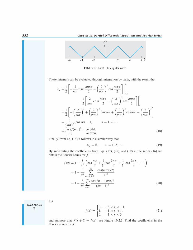
Determine the coefficients in this Fourier series.This function represents a triangular wave (see Figure 10.2.2) and is periodic with

period 4. Thus in this case L = 2 and the Fourier series has the form

f (x) = a02

+∞∑m=1

(am cos

mπx2

+ bm sinmπx2

), (16)

where the coefficients are computed from Eqs. (13) and (14) with L = 2. Substitutingfor f (x) in Eq. (13) with m = 0, we have

a0 = 12

∫ 0

−2(−x) dx + 1

2

∫ 2

0x dx = 1+ 1 = 2. (17)

For m > 0, Eq. (13) yields

am = 12

∫ 0

−2(−x) cos mπx

2dx + 1

2

∫ 2

0x cos

mπx2

dx .


x

y

–6 –4 –2 2

2

4 6

FIGURE 10.2.2 Triangular wave.

These integrals can be evaluated through integration by parts, with the result that

am = 12

[− 2mπ

x sinmπx2

−(2mπ

)2cos

mπx2

] ∣∣∣∣∣0

−2

+ 12

[2mπ

x sinmπx2

+(2mπ

)2cos

mπx2

] ∣∣∣∣∣2

0

= 12

[−

(2mπ

)2+

(2mπ

)2cosmπ +

(2mπ

)2cosmπ −

(2mπ

)2]

= 4(mπ)2

(cosmπ − 1), m = 1, 2, . . .

={−8/(mπ)2, m odd,0, m even. (18)

Finally, from Eq. (14) it follows in a similar way that

bm = 0, m = 1, 2, . . . . (19)

By substituting the coefficients from Eqs. (17), (18), and (19) in the series (16) weobtain the Fourier series for f :

f (x) = 1− 8π2

(cos

πx2

+ 132cos

3πx2

+ 152cos

5πx2

+ · · ·)

= 1− 8π2

∞∑m=1,3,5,...

cos(mπx/2)m2

= 1− 8π2

∞∑n=1

cos(2n − 1)πx/2(2n − 1)2 . (20)

E X A M P L E

2Let

f (x) =⎧⎨⎩0, −3 < x < −1,1, −1 < x < 1,0, 1 < x < 3

(21)

and suppose that f (x + 6) = f (x); see Figure 10.2.3. Find the coefficients in theFourier series for f .

10.2 Fourier Series 553y

t–7 –5 –3 –1 1

1

3 5 7

FIGURE 10.2.3 Graph of f (x) in Example 2.

Since f has period 6, it follows that L = 3 in this problem. Consequently, the Fourierseries for f has the form

f (x) = a02

+∞∑n=1

(an cos

nπx3

+ bn sinnπx3

), (22)

where the coefficients an and bn are given by Eqs. (13) and (14) with L = 3. We have

a0 = 13

∫ 3

−3f (x) dx = 1

3

∫ 1

−1dx = 2

3. (23)

Similarly,

an = 13

∫ 1

−1cos

nπx3dx = 1

nπsinnπx3

∣∣∣∣∣1

−1= 2nπsinnπ3

, n = 1, 2, . . . , (24)

and

bn = 13

∫ 1

−1sinnπx3dx = − 1

nπcos

nπx3

∣∣∣∣∣1

−1= 0, n = 1, 2, . . . . (25)

Thus the Fourier series for f is

f (x) = 13

+∞∑n=1

2nπsinnπ3cos

nπx3

= 13

+√3

π

[cos(πx/3) + cos(2πx/3)

2− cos(4πx/3)

4− cos(5πx/3)

5+ · · ·

].

(26)

E X A M P L E

3Consider again the function in Example 1 and its Fourier series (20). Investigate thespeed with which the series converges. In particular, determine how many terms areneeded so that the error is no greater than 0.01 for all x .The mth partial sum in this series,

sm(x) = 1− 8π2

m∑n=1

cos(2n − 1)πx/2(2n − 1)2 , (27)

can be used to approximate the function f . The coefficients diminish as (2n − 1)−2, sothe series converges fairly rapidly. This is borne out by Figure 10.2.4, where the partialsums for m = 1 and m = 2 are plotted. To investigate the convergence in more detail


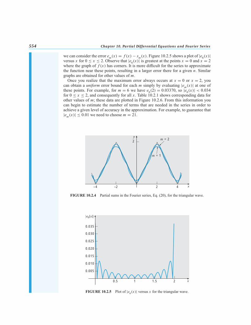
we can consider the error em(x) = f (x) − sm(x). Figure 10.2.5 shows a plot of |e6(x)|versus x for 0 ≤ x ≤ 2. Observe that |e6(x)| is greatest at the points x = 0 and x = 2where the graph of f (x) has corners. It is more difficult for the series to approximatethe function near these points, resulting in a larger error there for a given n. Similargraphs are obtained for other values of m.Once you realize that the maximum error always occurs at x = 0 or x = 2, you

can obtain a uniform error bound for each m simply by evaluating |em(x)| at one ofthese points. For example, for m = 6 we have e6(2) = 0.03370, so |e6(x)| < 0.034for 0 ≤ x ≤ 2, and consequently for all x . Table 10.2.1 shows corresponding data forother values of m; these data are plotted in Figure 10.2.6. From this information youcan begin to estimate the number of terms that are needed in the series in order toachieve a given level of accuracy in the approximation. For example, to guarantee that|em(x)| ≤ 0.01 we need to choose m = 21.

y

2

m = 2

m = 1

–4 –2

2

4 x

FIGURE 10.2.4 Partial sums in the Fourier series, Eq. (20), for the triangular wave.

x

0.025

0.020

0.015

0.010

0.005

e6(x)

0.030

0.035

1.51 20.5

FIGURE 10.2.5 Plot of |e6(x)| versus x for the triangular wave.


TABLE 10.2.1 Values of the Error em(2) forthe Triangular Wave

m em(2)

2 0.099374 0.050406 0.0337010 0.0202515 0.0135020 0.0101325 0.00810

m

0.08

0.06

0.04

0.02

em(2)

0.10

1510 20 255

FIGURE 10.2.6 Plot of em(2) versus m for the triangular wave.

In this book Fourier series appear mainly as a means of solving certain problemsin partial differential equations. However, such series have much wider applicationin science and engineering, and in general are valuable tools in the investigation ofperiodic phenomena. A basic problem is to resolve an incoming signal into its harmoniccomponents, which amounts to constructing its Fourier series representation. In somefrequency ranges the separate terms correspond to different colors or to different audibletones. The magnitude of the coefficient determines the amplitude of each component.This process is referred to as spectral analysis.

PROBLEMS In each of Problems 1 through 8 determine whether the given function is periodic. If so, find itsfundamental period.

1. sin 5x 2. cos 2πx3. sinh 2x 4. sinπx/L5. tanπx 6. x2

7. f (x) ={0, 2n − 1 ≤ x < 2n,1, 2n ≤ x < 2n + 1; n = 0, ±1, ±2, . . .

8. f (x) ={(−1)n, 2n − 1 ≤ x < 2n,1, 2n ≤ x < 2n + 1; n = 0, ±1, ±2, . . .


9. If f (x) = −x for −L < x < L , and if f (x + 2L) = f (x), find a formula for f (x) in theinterval L < x < 2L; in the interval −3L < x < −2L .

10. If f (x) ={x + 1, −1 < x < 0,x, 0 < x < 1, and if f (x + 2) = f (x), find a formula for f (x) in

the interval 1 < x < 2; in the interval 8 < x < 9.11. If f (x) = L − x for 0 < x < 2L , and if f (x + 2L) = f (x), find a formula for f (x) in

the interval −L < x < 0.12. Verify Eqs. (6) and (7) of the text by direct integration.

In each of Problems 13 through 18:(a) Sketch the graph of the given function for three periods.(b) Find the Fourier series for the given function.

13. f (x) = −x, −L ≤ x < L; f (x + 2L) = f (x)

14. f (x) ={1, −L ≤ x < 0,0, 0 ≤ x < L; f (x + 2L) = f (x)

15. f (x) ={x, −π ≤ x < 0,0, 0 ≤ x < π; f (x + 2π) = f (x)

16. f (x) ={x + 1, −1 ≤ x < 0,1− x, 0 ≤ x < 1; f (x + 2) = f (x)

17. f (x) ={x + L , −L ≤ x ≤ 0,L , 0 < x < L; f (x + 2L) = f (x)

18. f (x) =⎧⎨⎩0, −2 ≤ x ≤ −1,x, −1 < x < 1,0, 1 ≤ x < 2;

f (x + 4) = f (x)

In each of Problems 19 through 24:(a) Sketch the graph of the given function for three periods.(b) Find the Fourier series for the given function.(c) Plot sm(x) versus x for m = 5, 10, and 20.(d) Describe how the Fourier series seems to be converging.

� 19. f (x) ={−1, −2 ≤ x < 0,1, 0 ≤ x < 2; f (x + 4) = f (x)

� 20. f (x) = x, −1 ≤ x < 1; f (x + 2) = f (x)� 21. f (x) = x2/2, −2 ≤ x ≤ 2; f (x + 4) = f (x)

� 22. f (x) ={x + 2, −2 ≤ x < 0,2− 2x, 0 ≤ x < 2; f (x + 4) = f (x)

� 23. f (x) ={− 1

2 x, −2 ≤ x < 0,2x − 1

2 x2, 0 ≤ x < 2; f (x + 4) = f (x)

� 24. f (x) ={0, −3 ≤ x ≤ 0,x2(3− x), 0 < x < 3; f (x + 6) = f (x)

� 25. Consider the function f defined in Problem 21 and let em(x) = f (x) − sm(x). Plot |em(x)|versus x for 0 ≤ x ≤ 2 for several values of m. Find the smallest value of m for which|em(x)| ≤ 0.01 for all x .

� 26. Consider the function f defined in Problem 24 and let em(x) = f (x) − sm(x). Plot |em(x)|versus x for 0 ≤ x ≤ 3 for several values of m. Find the smallest value of m for which|em(x)| ≤ 0.1 for all x .

27. Suppose that g is an integrable periodic function with period T .


(a) If 0 ≤ a ≤ T , show that ∫ T

0g(x) dx =

∫ a+T

ag(x) dx .

Hint: Show first that∫ a

0g(x) dx =

∫ a+T

Tg(x) dx . Consider the change of variable s =

x − T in the second integral.(b) Show that for any value of a, not necessarily in 0 ≤ a ≤ T ,∫ T

0g(x) dx =

∫ a+T

ag(x) dx .

(c) Show that for any values of a and b,∫ a+T

ag(x) dx =

∫ b+T

bg(x) dx .

28. If f is differentiable and is periodic with period T , show that f ′ is also periodic withperiod T . Determine whether

F(x) =∫ x

0f (t) dt

is always periodic.29. In this problem we indicate certain similarities between three-dimensional geometric vec-

tors and Fourier series.(a) Let v1, v2, and v3 be a set of mutually orthogonal vectors in three dimensions and let ube any three-dimensional vector. Show that

u = a1v1 + a2v2 + a3v3, (i)

where

ai = u � vivi � vi

, i = 1, 2, 3. (ii)

Show that ai can be interpreted as the projection of u in the direction of vi divided by thelength of vi .(b) Define the inner product (u, v) by

(u, v) =∫ L

−Lu(x)v(x) dx . (iii)

Also let

φn(x) = cos(nπx/L), n = 0, 1, 2, . . . ;(iv)

ψn(x) = sin(nπx/L), n = 1, 2, . . . .

Show that Eq. (10) can be written in the form

( f, φn) = a02

(φ0, φn) +∞∑m=1

am(φm, φn) +∞∑m=1

bm(ψm, φn). (v)

(c) Use Eq. (v) and the corresponding equation for ( f, ψn) together with the orthogonalityrelations to show that

an = ( f, φn)(φn, φn)

, n = 0, 1, 2, . . . ; bn = ( f, ψn)(ψn, ψn)

, n = 1, 2, . . . . (vi)

Note the resemblance between Eqs. (vi) and Eq. (ii). The functions φn and ψn play a rolefor functions similar to that of the orthogonal vectors v1, v2, and v3 in three-dimensional


space. The coefficients an and bn can be interpreted as projections of the function f ontothe base functions φn and ψn .Observe also that any vector in three dimensions can be expressed as a linear combination

of three mutually orthogonal vectors. In a somewhat similar way any sufficiently smoothfunction defined on−L ≤ x ≤ L can be expressed as a linear combination of the mutuallyorthogonal functions cos(nπx/L) and sin(nπx/L), that is, as a Fourier series.

10.3 The Fourier Convergence TheoremIn the preceding section we showed that if the Fourier series

a02

+∞∑m=1

(am cos

mπxL

+ bm sinmπxL

)(1)

converges and thereby defines a function f , then f is periodic with period 2L , and thecoefficients am and bm are related to f (x) by the Euler–Fourier formulas:

am = 1L

∫ L

−Lf (x) cos

mπxL

dx, m = 0, 1, 2, . . . ; (2)

bm = 1L

∫ L

−Lf (x) sin

mπxL

dx, m = 1, 2, . . . . (3)

In this section we adopt a somewhat different point of view. Suppose that a functionf is given. If this function is periodic with period 2L and integrable on the interval[−L , L], then a set of coefficients am and bm can be computed from Eqs. (2) and (3),and a series of the form (1) can be formally constructed. The question is whether thisseries converges for each value of x and, if so, whether its sum is f (x). Examples havebeen discovered showing that the Fourier series corresponding to a function f may notconverge to f (x), or may even diverge. Functions whose Fourier series do not convergeto the value of the function at isolated points are easily constructed, and examples willbe presented later in this section. Functions whose Fourier series diverge at one or morepoints are more pathological, and we will not consider them in this book.To guarantee convergence of a Fourier series to the function from which its coef-

ficients were computed it is essential to place additional conditions on the function.From a practical point of view, such conditions should be broad enough to cover allsituations of interest, yet simple enough to be easily checked for particular functions.Through the years several sets of conditions have been devised to serve this purpose.Before stating a convergence theorem for Fourier series, we define a term that

appears in the theorem. A function f is said to be piecewise continuous on aninterval a ≤ x ≤ b if the interval can be partitioned by a finite number of pointsa = x0 < x1 < · · · < xn = b so that1. f is continuous on each open subinterval xi−1 < x < xi .2. f approaches a finite limit as the endpoints of each subinterval are approached

from within the subinterval.

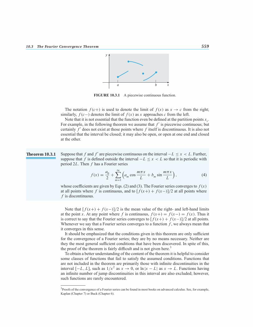
The graph of a piecewise continuous function is shown in Figure 10.3.1.

10.3 The Fourier Convergence Theorem 559y

xba

FIGURE 10.3.1 A piecewise continuous function.

The notation f (c+) is used to denote the limit of f (x) as x → c from the right;similarly, f (c−) denotes the limit of f (x) as x approaches c from the left.Note that it is not essential that the function even be defined at the partition points xi .

For example, in the following theorem we assume that f ′ is piecewise continuous; butcertainly f ′ does not exist at those points where f itself is discontinuous. It is also notessential that the interval be closed; it may also be open, or open at one end and closedat the other.

Theorem 10.3.1 Suppose that f and f ′ are piecewise continuous on the interval−L ≤ x < L . Further,suppose that f is defined outside the interval −L ≤ x < L so that it is periodic withperiod 2L . Then f has a Fourier series

f (x) = a02

+∞∑m=1

(am cos

mπxL

+ bm sinmπxL

), (4)

whose coefficients are given by Eqs. (2) and (3). The Fourier series converges to f (x)at all points where f is continuous, and to [ f (x+) + f (x−)]/2 at all points wheref is discontinuous.

Note that [ f (x+) + f (x−)]/2 is the mean value of the right- and left-hand limitsat the point x . At any point where f is continuous, f (x+) = f (x−) = f (x). Thus itis correct to say that the Fourier series converges to [ f (x+) + f (x−)]/2 at all points.Whenever we say that a Fourier series converges to a function f , we always mean thatit converges in this sense.It should be emphasized that the conditions given in this theorem are only sufficient

for the convergence of a Fourier series; they are by no means necessary. Neither arethey the most general sufficient conditions that have been discovered. In spite of this,the proof of the theorem is fairly difficult and is not given here.3To obtain a better understanding of the content of the theorem it is helpful to consider

some classes of functions that fail to satisfy the assumed conditions. Functions thatare not included in the theorem are primarily those with infinite discontinuities in theinterval [−L , L], such as 1/x2 as x → 0, or ln |x − L| as x → L . Functions havingan infinite number of jump discontinuities in this interval are also excluded; however,such functions are rarely encountered.

3Proofs of the convergence of a Fourier series can be found in most books on advanced calculus. See, for example,Kaplan (Chapter 7) or Buck (Chapter 6).


It is noteworthy that a Fourier series may converge to a sum that is not differentiable,or even continuous, in spite of the fact that each term in the series (4) is continuous,and even differentiable infinitely many times. The example below is an illustration ofthis, as is Example 2 in Section 10.2.

E X A M P L E

1Let

f (x) ={0, −L < x < 0,L , 0 < x < L ,

(5)

and let f be defined outside this interval so that f (x + 2L) = f (x) for all x . We willtemporarily leave open the definition of f at the points x = 0,±L , except that itsvalue must be finite. Find the Fourier series for this function and determine where itconverges.

y

x3L2LL

L

–L–2L–3L

FIGURE 10.3.2 Square wave.

The equation y = f (x) has the graph shown in Figure 10.3.2, extended to infinityin both directions. It can be thought of as representing a square wave. The interval[−L , L] can be partitioned to give the two open subintervals (−L , 0) and (0, L). In(0, L), f (x) = L and f ′(x) = 0.Clearly, both f and f ′ are continuous and furthermorehave limits as x → 0 from the right and as x → L from the left. The situation in (−L , 0)is similar. Consequently, both f and f ′ are piecewise continuous on [−L , L), so fsatisfies the conditions of Theorem 10.3.1. If the coefficients am and bm are computedfrom Eqs. (2) and (3), the convergence of the resulting Fourier series to f (x) is assuredat all points where f is continuous. Note that the values of am and bm are the sameregardless of the definition of f at its points of discontinuity. This is true because thevalue of an integral is unaffected by changing the value of the integrand at a finitenumber of points. From Eq. (2)

a0 = 1L

∫ L

−Lf (x) dx =

∫ L

0dx = L;

am = 1L

∫ L

−Lf (x) cos

mπxL

dx =∫ L

0cos

mπxL

dx

= 0, m �= 0.

Similarly, from Eq. (3),

bm = 1L

∫ L

−Lf (x) sin

mπxL

dx =∫ L

0sinmπxL

dx

= Lmπ

(1− cosmπ)

={0, m even;2L/mπ, m odd.

10.3 The Fourier Convergence Theorem 561

Hence

f (x) = L2

+ 2Lπ

(sin

πxL

+ 13sin3πxL

+ 15sin5πxL

+ · · ·)

= L2

+ 2Lπ

∞∑m=1,3,5,...

sin(mπx/L)

m

= L2

+ 2Lπ

∞∑n=1

sin(2n − 1)πx/L2n − 1 . (6)

At the points x = 0, ±nL , where the function f in the example is not continuous,all terms in the series after the first vanish and the sum is L/2. This is the mean valueof the limits from the right and left, as it should be. Thus we might as well define fat these points to have the value L/2. If we choose to define it otherwise, the seriesstill gives the value L/2 at these points, since none of the preceding calculations isaltered in any detail; it simply does not converge to the function at those points unlessf is defined to have this value. This illustrates the possibility that the Fourier seriescorresponding to a function may not converge to it at points of discontinuity unless thefunction is suitably defined at such points.The manner in which the partial sums

sn(x) = L2

+ 2Lπ

(sin

πxL

+ · · · + 12n − 1 sin

(2n − 1)πxL

), n = 1, 2, . . .

of the Fourier series (6) converge to f (x) is indicated in Figure 10.3.3, where L hasbeen chosen to be one and the graph of s8(x) is plotted. The figure suggests that at pointswhere f is continuous the partial sums do approach f (x) as n increases. However, inthe neighborhood of points of discontinuity, such as x = 0 and x = L , the partial sumsdo not converge smoothly to the mean value. Instead they tend to overshoot the markat each end of the jump, as though they cannot quite accommodate themselves to thesharp turn required at this point. This behavior is typical of Fourier series at points ofdiscontinuity, and is known as the Gibbs4 phenomenon.

y

x–2 2–1 1

1 n = 8

FIGURE 10.3.3 The partial sum s8(x) in the Fourier series, Eq. (6), for the square wave.

Additional insight is attained by considering the error en(x) = f (x) − sn(x). Figure10.3.4 shows a plot of |en(x)| versus x for n = 8 and for L = 1. The least upper boundof |e8(x)| is 0.5 and is approached as x → 0 and as x → 1. As n increases, the error

4The Gibbs phenomenon is named after Josiah Willard Gibbs (1839–1903), who is better known for his work onvector analysis and statistical mechanics. Gibbs was professor of mathematical physics at Yale, and one of thefirst American scientists to achieve an international reputation. Gibbs’ phenomenon is discussed in more detailby Carslaw (Chapter 9).


decreases in the interior of the interval [where f (x) is continuous] but the least upperbound does not diminish with increasing n. Thus one cannot uniformly reduce the errorthroughout the interval by increasing the number of terms.Figures 10.3.3 and 10.3.4 also show that the series in this example converges more

slowly than the one in Example 1 in Section 10.2. This is due to the fact that thecoefficients in the series (6) are proportional only to 1/(2n − 1).

10.4 0.60.2 0.8

0.4

0.3

0.2

0.1

x

e8(x)0.5

FIGURE 10.3.4 A plot of the error |e8(x)| versus x for the square wave.

PROBLEMS In each of Problems 1 through 6 assume that the given function is periodically extended outsidethe original interval.

(a) Find the Fourier series for the extended function.(b) Sketch the graph of the function to which the series converges for three periods.

1. f (x) ={−1, −1 ≤ x < 0,1, 0 ≤ x < 1 2. f (x) =

{0, −π ≤ x < 0,x, 0 ≤ x < π

3. f (x) ={L + x, −L ≤ x < 0,L − x, 0 ≤ x < L 4. f (x) = 1− x2, −1 ≤ x ≤ 1

5. f (x) =⎧⎨⎩0, −π ≤ x < −π/2,1, −π/2 ≤ x < π/2,0, π/2 ≤ x < π

6. f (x) ={0, −1 ≤ x < 0,x2, 0 ≤ x < 1

In each of Problems 7 through 12 assume that the given function is periodically extended outsidethe original interval.(a) Find the Fourier series for the given function.(b) Let en(x) = f (x) − sn(x). Find the least upper bound or the maximum value (if it exists)

of |en(x)| for n = 10, 20, and 40.(c) If possible, find the smallest n for which |en(x)| ≤ 0.01 for all x .

� 7. f (x) ={x, −π ≤ x < 0,0, 0 ≤ x < π; f (x + 2π) = f (x) (see Section 10.2, Problem 15)

10.3 The Fourier Convergence Theorem 563

� 8. f (x) ={x + 1, −1 ≤ x < 0,1− x, 0 ≤ x < 1; f (x + 2) = f (x) (see Section 10.2, Problem 16)

� 9. f (x) = x, −1 ≤ x < 1; f (x + 2) = f (x) (see Section 10.2, Problem 20)

� 10. f (x) ={x + 2, −2 ≤ x < 0,2− 2x, 0 ≤ x < 2; f (x + 4) = f (x) (see Section 10.2,

Problem 22)

� 11. f (x) ={0, −1 ≤ x < 0,x2, 0 ≤ x < 1; f (x + 2) = f (x) (see Problem 6)

� 12. f (x) = x − x3, −1 ≤ x < 1; f (x + 2) = f (x)

Periodic ForcingTerms. In this chapterwe are concernedmainlywith the use of Fourier seriesto solve boundary value problems for certain partial differential equations. However, Fourierseries are also useful in many other situations where periodic phenomena occur. Problems 13through 16 indicate how they can be employed to solve initial value problems with periodicforcing terms.

13. Find the solution of the initial value problem

y′′ + ω2y = sin nt, y(0) = 0, y′(0) = 0,where n is a positive integer and ω2 �= n2. What happens if ω2 = n2?

14. Find the formal solution of the initial value problem

y′′ + ω2y =∞∑n=1bn sin nt, y(0) = 0, y′(0) = 0,

where ω > 0 is not equal to a positive integer. How is the solution altered if ω = m, wherem is a positive integer?

15. Find the formal solution of the initial value problem

y′′ + ω2y = f (t), y(0) = 0, y′(0) = 0,

where f is periodic with period 2π and

f (t) =⎧⎨⎩

1, 0 < t < π;0, t = 0, π, 2π;

−1, π < t < 2π.

See Problem 1.16. Find the formal solution of the initial value problem

y′′ + ω2y = f (t), y(0) = 1, y′(0) = 0,

where f is periodic with period 2 and

f (t) ={1− t, 0 ≤ t < 1;

−1+ t, 1 ≤ t < 2.

See Problem 8.17. Assuming that

f (x) = a02

+∞∑n=1

(an cos

nπxL

+ bn sinnπxL

), (i)

show formally that

1L

∫ L

−L[ f (x)]2 dx = a20

2+

∞∑n=1

(a2n + b2n).


This relation between a function f and its Fourier coefficients is known as Parseval’s(1755–1836) equation. Parseval’s equation is very important in the theory of Fourier seriesand is discussed further in Section 11.6.Hint:Multiply Eq. (i) by f (x), integrate from−L to L , and use the Euler–Fourier formulas.

18. This problem indicates a proof of convergence of a Fourier series under conditions morerestrictive than those in Theorem 10.3.1.(a) If f and f ′ are piecewise continuous on−L ≤ x < L , and if f is periodic with period2L , show that nan and nbn are bounded as n → ∞.Hint: Use integration by parts.(b) If f is continuous on −L ≤ x ≤ L and periodic with period 2L , and if f ′ and f ′′ arepiecewise continuous on −L ≤ x < L , show that n2an and n

2bn are bounded as n → ∞.Use this fact to show that the Fourier series for f converges at each point in −L ≤ x ≤ L .Why must f be continuous on the closed interval?Hint: Again, use integration by parts.Acceleration of Convergence. In the next problemwe show how it is sometimes possibleto improve the speed of convergence of a Fourier, or other infinite, series.

19. Suppose that we wish to calculate values of the function g, where

g(x) =∞∑n=1

(2n − 1)1+ (2n − 1)2 sin(2n − 1)πx . (i)

It is possible to show that this series converges, albeit rather slowly. However, observe thatfor large n the terms in the series (i) are approximately equal to [sin(2n − 1)πx]/(2n − 1)and that the latter terms are similar to those in the example in the text, Eq. (6).(a) Show that

∞∑n=1[sin(2n − 1)πx]/(2n − 1) = (π/2)[ f (x) − 1

2 ], (ii)

where f is the square wave in the example with L = 1.(b) Subtract Eq. (ii) from Eq. (i) and show that

g(x) = π

2[ f (x) − 1

2 ]−∞∑n=1

sin(2n − 1)πx(2n − 1)[1+ (2n − 1)2] . (iii)

The series (iii) converges much faster than the series (i) and thus provides a better way tocalculate values of g(x).

10.4 Even and Odd FunctionsBefore looking at further examples of Fourier series it is useful to distinguish twoclasses of functions for which the Euler–Fourier formulas can be simplified. Theseare even and odd functions, which are characterized geometrically by the property ofsymmetry with respect to the y-axis and the origin, respectively (see Figure 10.4.1).Analytically, f is an even function if its domain contains the point −x whenever it

contains the point x , and if

f (−x) = f (x) (1)

10.4 Even and Odd Functions 565

y y

xx

(a) (b)

FIGURE 10.4.1 (a) An even function. (b) An odd function.

for each x in the domain of f . Similarly, f is an odd function if its domain contains−x whenever it contains x , and if

f (−x) = − f (x) (2)

for each x in the domain of f . Examples of even functions are 1, x2, cos nx , |x |, andx2n . The functions x , x3, sin nx , and x2n+1 are examples of odd functions. Note thataccording to Eq. (2), f (0)must be zero if f is an odd function whose domain containsthe origin. Most functions are neither even nor odd, for instance, ex . Only one function,f identically zero, is both even and odd.Elementary properties of even and odd functions include the following:

1. The sum (difference) and product (quotient) of two even functions are even.2. The sum (difference) of two odd functions is odd; the product (quotient) of two

odd functions is even.3. The sum (difference) of an odd function and an even function is neither even nor

odd; the product (quotient) of two such functions is odd.5

The proofs of all these assertions are simple and follow directly from the definitions.For example, if both f1 and f2 are odd, and if g(x) = f1(x) + f2(x), then

g(−x) = f1(−x) + f2(−x) = − f1(x) − f2(x)= −[ f1(x) + f2(x)] = −g(x), (3)

so f1 + f2 is an odd function also. Similarly, if h(x) = f1(x) f2(x), then

h(−x) = f1(−x) f2(−x) = [− f1(x)][− f2(x)] = f1(x) f2(x) = h(x), (4)

so that f1 f2 is even.Also of importance are the following two integral properties of even and odd

functions:4. If f is an even function, then∫ L

−Lf (x) dx = 2

∫ L

0f (x) dx . (5)

5These statements may need to be modified if either function vanishes identically.


5. If f is an odd function, then ∫ L

−Lf (x) dx = 0. (6)

These properties are intuitively clear from the interpretation of an integral in termsof area under a curve, and also follow immediately from the definitions. For example,if f is even, then ∫ L

−Lf (x) dx =

∫ 0

−Lf (x) dx +

∫ L

0f (x) dx .

Letting x = −s in the first term on the right side, and using Eq. (1), we obtain∫ L

−Lf (x) dx = −

∫ 0

Lf (s) ds +

∫ L

0f (x) dx = 2

∫ L

0f (x) dx .

The proof of the corresponding property for odd functions is similar.Even and odd functions are particularly important in applications of Fourier se-

ries since their Fourier series have special forms, which occur frequently in physicalproblems.

Cosine Series. Suppose that f and f ′ are piecewise continuous on−L ≤ x < L , andthat f is an even periodic function with period 2L . Then it follows from properties 1and 3 that f (x) cos(nπx/L) is even and f (x) sin(nπx/L) is odd. As a consequenceof Eqs. (5) and (6), the Fourier coefficients of f are then given by

an = 2L

∫ L

0f (x) cos

nπxL

dx, n = 0, 1, 2, . . . ;(7)

bn = 0, n = 1, 2, . . . .

Thus f has the Fourier series

f (x) = a02

+∞∑n=1an cos

nπxL

.

In other words, the Fourier series of any even function consists only of the eventrigonometric functions cos(nπx/L) and the constant term; it is natural to call such aseries a Fourier cosine series. From a computational point of view, observe that onlythe coefficients an , for n = 0, 1, 2, . . . , need to be calculated from the integral formula(7). Each of the bn , for n = 1, 2, . . . , is automatically zero for any even function, andso does not need to be calculated by integration.

Sine Series. Suppose that f and f ′ are piecewise continuous on −L ≤ x < L , andthat f is an odd periodic function of period 2L . Then it follows from properties 2 and3 that f (x) cos(nπx/L) is odd and f (x) sin(nπx/L) is even. In this case the Fouriercoefficients of f are

an = 0, n = 0, 1, 2, . . . ,(8)

bn = 2L

∫ L

0f (x) sin

nπxL

dx, n = 1, 2, . . . ,


and the Fourier series for f is of the form

f (x) =∞∑n=1bn sin

nπxL

.

Thus the Fourier series for any odd function consists only of the odd trigonometricfunctions sin(nπx/L); such a series is called a Fourier sine series. Again observe thatonly half of the coefficients need to be calculated by integration, since each an , forn = 0, 1, 2, . . . , is zero for any odd function.

E X A M P L E

1Let f (x) = x ,−L < x < L , and let f (−L) = f (L) = 0. Let f be defined elsewhereso that it is periodic of period 2L (see Figure 10.4.2). The function defined in thismanner is known as a sawtooth wave. Find the Fourier series for this function.Since f is an odd function, its Fourier coefficients are, according to Eq. (8),

an = 0, n = 0, 1, 2, . . . ;

bn = 2L

∫ L

0x sin

nπxL

dx

= 2L

(Lnπ

)2 {sinnπxL

− nπxLcos

nπxL

}∣∣∣∣∣L

0

= 2Lnπ

(−1)n+1, n = 1, 2, . . . .

Hence the Fourier series for f , the sawtooth wave, is

f (x) = 2Lπ

∞∑n=1

(−1)n+1n

sinnπxL

. (9)

Observe that the periodic function f is discontinuous at the points ±L ,±3L , . . . , asshown in Figure 10.4.2. At these points the series (9) converges to the mean value ofthe left and right limits, namely, zero. The partial sum of the series (9) for n = 9 isshown in Figure 10.4.3. The Gibbs phenomenon (mentioned in Section 10.3) againoccurs near the points of discontinuity.

x

y

L

–3L –2L

–L

–L L 2L 3L

FIGURE 10.4.2 Sawtooth wave.


y

x–2L –L L

–L

L

2L

n = 9

FIGURE 10.4.3 A partial sum in the Fourier series, Eq. (9), for the sawtooth wave.

Note that in this example f (−L) = f (L) = 0, as well as f (0) = 0. This is requiredif the function f is to be both odd and periodic with period 2L . When we speak ofconstructing a sine series for a function defined on 0 ≤ x ≤ L , it is understood that, ifnecessary, we must first redefine the function to be zero at x = 0 and x = L .It is worthwhile to observe that the triangular wave function (Example 1 of Section

10.2) and the sawtooth wave function just considered are identical on the interval0 ≤ x < L . Therefore, their Fourier series converge to the same function, f (x) = x ,on this interval. Thus, if it is required to represent the function f (x) = x on 0 ≤ x < Lby a Fourier series, it is possible to do this by either a cosine series or a sine series.In the former case f is extended as an even function into the interval −L < x < 0and elsewhere periodically (the triangular wave). In the latter case f is extended into−L < x < 0 as an odd function, and elsewhere periodically (the sawtooth wave). Iff is extended in any other way, the resulting Fourier series will still converge to x in0 ≤ x < L but will involve both sine and cosine terms.In solving problems in differential equations it is often useful to expand in a Fourier

series of period 2L a function f originally defined only on the interval [0, L]. As indi-cated previously for the function f (x) = x several alternatives are available. Explicitly,we can:

1. Define a function g of period 2L so that

g(x) ={f (x), 0 ≤ x ≤ L ,

f (−x), −L < x < 0. (10)

The function g is thus the even periodic extension of f . Its Fourier series, whichis a cosine series, represents f on [0, L].

2. Define a function h of period 2L so that

h(x) =⎧⎨⎩

f (x), 0 < x < L ,

0, x = 0, L ,

− f (−x), −L < x < 0.(11)

The function h is thus the odd periodic extension of f . Its Fourier series, which isa sine series, also represents f on (0, L).


3. Define a function k of period 2L so that

k(x) = f (x), 0 ≤ x ≤ L , (12)

and let k(x) be defined for (−L , 0) in any way consistent with the conditionsof Theorem 10.3.1. Sometimes it is convenient to define k(x) to be zero for−L < x < 0. The Fourier series for k, which involves both sine and cosine terms,also represents f on [0, L], regardless of the manner in which k(x) is defined in(−L , 0). Thus there are infinitely many such series, all of which converge to f (x)in the original interval.

Usually, the form of the expansion to be used will be dictated (or at least suggested)by the purpose for which it is needed. However, if there is a choice as to the kindof Fourier series to be used, the selection can sometimes be based on the rapidity ofconvergence. For example, the cosine series for the triangular wave [Eq. (20) of Section10.2] converges more rapidly than the sine series for the sawtooth wave [Eq. (9) in thissection], although both converge to the same function for 0 ≤ x < L . This is due tothe fact that the triangular wave is a smoother function than the sawtooth wave and istherefore easier to approximate. In general, the more continuous derivatives possessedby a function over the entire interval −∞ < x < ∞, the faster its Fourier series willconverge. See Problem 18 of Section 10.3.

E X A M P L E

2Suppose that

f (x) ={1− x, 0 < x ≤ 1,0, 1 < x ≤ 2. (13)

As indicated previously, we can represent f either by a cosine series or by a sine series.Sketch the graph of the sum of each of these series for −6 ≤ x ≤ 6.In this example L = 2, so the cosine series for f converges to the even periodic

extension of f of period 4, whose graph is sketched in Figure 10.4.4.Similarly, the sine series for f converges to the odd periodic extension of f of

period 4. The graph of this function is shown in Figure 10.4.5.

x

y

–6 –4 –2–1

1

2 4 6

FIGURE 10.4.4 Even periodic extension of f (x) given by Eq. (13).

x

y

–6 –4 –2–1

1

2 4 6

FIGURE 10.4.5 Odd periodic extension of f (x) given by Eq. (13).


PROBLEMS In each of Problems 1 through 6 determine whether the given function is even, odd, or neither.

1. x3 − 2x 2. x3 − 2x + 1 3. tan 2x4. sec x 5. |x |3 6. e−x

In each of Problems 7 through 12 a function f is given on an interval of length L . In each casesketch the graphs of the even and odd extensions of f of period 2L .

7. f (x) ={x, 0 ≤ x < 2,1, 2 ≤ x < 3 8. f (x) =

{0, 0 ≤ x < 1,x − 1, 1 ≤ x < 2

9. f (x) = 2− x, 0 < x < 2 10. f (x) = x − 3, 0 < x < 4

11. f (x) ={0, 0 ≤ x < 1,1, 1 ≤ x < 2 12. f (x) = 4− x2, 0 < x < 1

13. Prove that any function can be expressed as the sum of two other functions, one of which iseven and the other odd. That is, for any function f , whose domain contains −x wheneverit contains x , show that there is an even function g and an odd function h such thatf (x) = g(x) + h(x).Hint: Assuming f (x) = g(x) + h(x), what is f (−x)?

14. Find the coefficients in the cosine and sine series described in Example 2.

In each of Problems 15 through 22 find the required Fourier series for the given function andsketch the graph of the function to which the series converges over three periods.

15. f (x) ={1, 0 < x < 1,0, 1 < x < 2; cosine series, period 4

Compare with Example 1 and Problem 5 of Section 10.3.

16. f (x) ={x, 0 ≤ x < 1,1, 1 ≤ x < 2; sine series, period 4

17. f (x) = 1, 0 ≤ x ≤ π; cosine series, period 2π18. f (x) = 1, 0 < x < π; sine series, period 2π

19. f (x) =⎧⎨⎩0, 0 < x < π,

1, π < x < 2π,

2, 2π < x < 3πsine series, period 6π

20. f (x) = x, 0 ≤ x < 1; series of period 121. f (x) = L − x, 0 ≤ x ≤ L; cosine series, period 2L

Compare with Example 1 of Section 10.2.22. f (x) = L − x, 0 < x < L; sine series, period 2L

In each of Problems 23 through 26:(a) Find the required Fourier series for the given function.(b) Sketch the graph of the function to which the series converges for three periods.(c) Plot one or more partial sums of the series.

� 23. f (x) ={x, 0 < x < π,

0, π < x < 2π; cosine series, period 4π

� 24. f (x) = −x, −π < x < 0; sine series, period 2π� 25. f (x) = 2− x2, 0 < x < 2; sine series, period 4� 26. f (x) = x2 − 2x, 0 < x < 4; cosine series, period 8

In each of Problems 27 through 30 a function is given on an interval 0 < x < L .(a) Sketch the graphs of the even extension g(x) and the odd extension h(x) of the given

function of period 2L over three periods.


(b) Find the Fourier cosine and sine series for the given function.(c) Plot a few partial sums of each series.(d) For each series investigate the dependence on n of the maximum error on [0, L].

� 27. f (x) = 3− x, 0 < x < 3 � 28. f (x) ={x, 0 < x < 1,0, 1 < x < 2

� 29. f (x) = (4x2 − 4x − 3)/4, 0 < x < 2

� 30. f (x) = x3 − 5x2 + 5x + 1, 0 < x < 3

31. Prove that if f is an odd function, then∫ L

−Lf (x) dx = 0.

32. Prove properties 2 and 3 of even and odd functions, as stated in the text.33. Prove that the derivative of an even function is odd, and that the derivative of an odd

function is even.

34. Let F(x) =∫ x

0f (t) dt . Show that if f is even, then F is odd, and that if f is odd, then

F is even.35. From the Fourier series for the square wave in Example 1 of Section 10.3, show that

π

4= 1− 1

3+ 15

− 17

+ · · · =∞∑n=0

(−1)n2n + 1 .

This relation between π and the odd positive integers was discovered by Leibniz in 1674.36. From the Fourier series for the triangular wave (Example 1 of Section 10.2), show that

π2

8= 1+ 1

32+ 152

+ · · · =∞∑n=0

1(2n + 1)2 .

37. Assume that f has a Fourier sine series

f (x) =∞∑n=1bn sin(nπx/L), 0 ≤ x ≤ L .

(a) Show formally that

2L

∫ L

0[ f (x)]2 dx =

∞∑n=1b2n .

Compare this result with that of Problem 17 in Section 10.3. What is the correspondingresult if f has a cosine series?(b) Apply the result of part (a) to the series for the sawtooth wave given in Eq. (9), andthereby show that

π2

6= 1+ 1

22+ 132

+ · · · =∞∑n=1

1n2

.

This relation was discovered by Euler about 1735.

More Specialized Fourier Series. Let f be a function originally defined on 0 ≤ x ≤ L . In thissection we have shown that it is possible to represent f either by a sine series or by a cosineseries by constructing odd or even periodic extensions of f , respectively. Problems 38 through40 concern some other more specialized Fourier series that converge to the given function fon (0, L).


38. Let f be extended into (L , 2L] in an arbitrary manner. Then extend the resulting functioninto (−2L , 0) as an odd function and elsewhere as a periodic function of period 4L (seeFigure 10.4.6). Show that this function has a Fourier sine series in terms of the functionssin(nπx/2L), n = 1, 2, 3, . . . ; that is,

f (x) =∞∑n=1bn sin(nπx/2L),

where

bn = 1L

∫ 2L

0f (x) sin(nπx/2L) dx .

This series converges to the original function on (0, L).

y

x2LL

–L–2L

FIGURE 10.4.6 Graph of the func-tion in Problem 38.

y

x2LL– L–2L

FIGURE 10.4.7 Graph of the func-tion in Problem 39.

39. Let f first be extended into (L , 2L) so that it is symmetric about x = L; that is, so asto satisfy f (2L − x) = f (x) for 0 ≤ x < L . Let the resulting function be extended into(−2L , 0) as an odd function and elsewhere (see Figure 10.4.7) as a periodic function ofperiod 4L . Show that this function has a Fourier series in terms of the functions sin(πx/2L),sin(3πx/2L), sin(5πx/2L), . . . ; that is,

f (x) =∞∑n=1bn sin

(2n − 1)πx2L

,

where

bn = 2L

∫ L

0f (x) sin

(2n − 1)πx2L

dx .

This series converges to the original function on (0, L].40. How should f , originally defined on [0, L], be extended so as to obtain a Fourier se-

ries involving only the functions cos(πx/2L), cos(3πx/2L), cos(5πx/2L), . . .? Refer toProblems 38 and 39. If f (x) = x for 0 ≤ x ≤ L , sketch the function to which the Fourierseries converges for −4L ≤ x ≤ 4L .

10.5 Separation of Variables; Heat Conduction in a Rod 573

10.5 Separation of Variables; Heat Conduction in a RodThe basic partial differential equations of heat conduction, wave propagation, and po-tential theory that we discuss in this chapter are associated with three distinct typesof physical phenomena: diffusive processes, oscillatory processes, and time indepen-dent or steady processes. Consequently, they are of fundamental importance in manybranches of physics. They are also of considerable significance from a mathemati-cal point of view. The partial differential equations whose theory is best developedand whose applications are most significant and varied are the linear equations ofsecond order. All such equations can be classified into one of three categories; theheat conduction equation, the wave equation, and the potential equation, respectively,are prototypes of each of these categories. Thus a study of these three equationsyields much information about more general second order linear partial differentialequations.During the last two centuries several methods have been developed for solving partial

differential equations. The method of separation of variables is the oldest systematicmethod, having been used by D’Alembert, Daniel Bernoulli, and Euler in about 1750in their investigations of waves and vibrations. It has been considerably refined andgeneralized in the meantime, and remains a method of great importance and frequentuse today. To show how the method of separation of variables works we considerfirst a basic problem of heat conduction in a solid body. The mathematical study ofheat conduction originated6 about 1800, and it continues to command the attentionof modern scientists. For example, the analysis of the dissipation and transfer of heataway from its sources in high-speedmachinery is frequently an important technologicalproblem.Let us now consider a heat conduction problem for a straight bar of uniform cross

section and homogeneous material. Let the x-axis be chosen to lie along the axisof the bar, and let x = 0 and x = L denote the ends of the bar (see Figure 10.5.1).Suppose further that the sides of the bar are perfectly insulated so that no heat passesthrough them. We also assume that the cross-sectional dimensions are so small that thetemperature u can be considered as constant on any given cross section. Then u is afunction only of the axial coordinate x and the time t .

x

u(x, t)

x = 0 x = L

FIGURE 10.5.1 A heat-conducting solid bar.

6The first important investigation of heat conduction was carried out by Joseph Fourier (1768–1830) while hewas serving as prefect of the department of Isere (Grenoble) from 1801 to 1815. He presented basic papers onthe subject to the Academy of Sciences of Paris in 1807 and 1811. However, these papers were criticized by thereferees (principally Lagrange) for lack of rigor and so were not published. Fourier continued to develop his ideasand eventually wrote one of the classics of applied mathematics, Theorie analytique de la chaleur, published in1822.


The variation of temperature in the bar is governed by a partial differential equationwhose derivation appears in Appendix A at the end of the chapter. The equation iscalled the heat conduction equation, and has the form

α2uxx = ut , 0 < x < L , t > 0, (1)

where α2 is a constant known as the thermal diffusivity. The parameter α2 dependsonly on the material from which the bar is made, and is defined by

α2 = κ/ρs, (2)

where κ is the thermal conductivity, ρ is the density, and s is the specific heat of thematerial in the bar. The units of α2 are (length)2/time. Typical values of α2 are givenin Table 10.5.1.

TABLE 10.5.1 Values of the ThermalDiffusivity for Some Common Materials

Material α2(cm2/sec)

Silver 1.71Copper 1.14Aluminum 0.86Cast iron 0.12Granite 0.011Brick 0.0038Water 0.00144

In addition, we assume that the initial temperature distribution in the bar is given;thus

u(x, 0) = f (x), 0 ≤ x ≤ L , (3)

where f is a given function. Finally, we assume that the ends of the bar are held at fixedtemperatures: the temperature T1 at x = 0 and the temperature T2 at x = L . However,it turns out that we need only consider the case where T1 = T2 = 0.We show in Section10.6 how to reduce the more general problem to this special case. Thus in this sectionwe will assume that u is always zero when x = 0 or x = L:

u(0, t) = 0, u(L , t) = 0, t > 0. (4)

The fundamental problem of heat conduction is to find u(x, t) that satisfies the differ-ential equation (1) for 0 < x < L and for t > 0, the initial condition (3) when t = 0,and the boundary conditions (4) at x = 0 and x = L .The problem described by Eqs. (1), (3), and (4) is an initial value problem in the

time variable t ; an initial condition is given and the differential equation governswhat happens later. However, with respect to the space variable x , the problem isa boundary value problem; boundary conditions are imposed at each end of the barand the differential equation describes the evolution of the temperature in the intervalbetween them. Alternatively, we can consider the problem as a boundary value problemin the xt-plane (see Figure 10.5.2). The solution u(x, t) of Eq. (1) is sought in the semi-infinite strip 0 < x < L , t > 0 subject to the requirement that u(x, t) must assume aprescribed value at each point on the boundary of this strip.


x

tx = L

u(0, t) = 0

u(x,0) = f (x)

u(L, t) = 02uxx = utα

FIGURE 10.5.2 Boundary value problem for the heat conduction equation.

The heat conduction problem (1), (3), (4) is linear since u appears only to thefirst power throughout. The differential equation and boundary conditions are alsohomogeneous. This suggests that we might approach the problem by seeking solutionsof the differential equation and boundary conditions, and then superposing them tosatisfy the initial condition. The remainder of this section describes how this plan canbe implemented.One solution of the differential equation (1) that satisfies the boundary conditions

(4) is the function u(x, t) = 0, but this solution does not satisfy the initial condition(3) except in the trivial case in which f (x) is also zero. Thus our goal is to find other,nonzero, solutions of the differential equation and boundary conditions. To find theneeded solutions, we start by making a basic assumption about the form of the solutionsthat has far-reaching, and perhaps unforeseen, consequences. The assumption is thatu(x, t) is a product of two other functions, one depending only on x and the otherdepending only on t ; thus

u(x, t) = X (x)T (t). (5)

Substituting from Eq. (5) for u in the differential equation (1) yields

α2X ′′T = XT ′, (6)

where primes refer to ordinary differentiation with respect to the independent variable,whether x or t . Equation (6) is equivalent to

X ′′

X= 1

α2T ′

T, (7)

in which the variables are separated; that is, the left side depends only on x and the rightside only on t . For Eq. (7) to be valid for 0 < x < L , t > 0, it is necessary that bothsides of Eq. (7) be equal to the same constant. Otherwise, by keeping one independentvariable (say, x) fixed and varying the other, one side (the left in this case) of Eq. (7)would remain unchanged while the other varied, thus violating the equality. If we callthis separation constant −λ, then Eq. (7) becomes

X ′′

X= 1

α2T ′

T= −λ. (8)


Hence we obtain the following two ordinary differential equations for X (x) and T (t):

X ′′ + λX = 0, (9)T ′ + α2λT = 0. (10)

We denote the separation constant by −λ (rather than λ) because it turns out that itmust be negative, and it is convenient to exhibit the minus sign explicitly.The assumption (5) has led to the replacement of the partial differential equation (1)

by the two ordinary differential equations (9) and (10). Each of these equations can bereadily solved for any value of λ. The product of two solutions of Eq. (9) and (10),respectively, provides a solution of the partial differential equation (1). However, weare interested only in those solutions of Eq. (1) that also satisfy the boundary conditions(4). As we now show, this severely restricts the possible values of λ.Substituting for u(x, t) from Eq. (5) in the boundary condition at x = 0, we obtain

u(0, t) = X (0)T (t) = 0. (11)

If Eq. (11) is satisfied by choosing T (t) to be zero for all t , then u(x, t) is zero forall x and t , and we have already rejected this possibility. Therefore Eq. (11) must besatisfied by requiring that

X (0) = 0. (12)

Similarly, the boundary condition at x = L requires that

X (L) = 0. (13)

We now want to consider Eq. (9) subject to the boundary conditions (12) and (13).This is an eigenvalue problem and, in fact, is the same problem that we discussed indetail at the end of Section 10.1; see especially the paragraph following Eq. (29) in thatsection. The only difference is that the dependent variable there was called y ratherthan X . If we refer to the results obtained earlier [Eq. (31) of Section 10.1], the onlynontrivial solutions of Eqs. (9), (12), and (13) are the eigenfunctions

Xn(x) = sin(nπx/L), n = 1, 2, 3, . . . , (14)

associated with the eigenvalues

λn = n2π2/L2, n = 1, 2, 3, . . . . (15)

Turning now to Eq. (10) for T (t) and substituting n2π2/L2 for λ, we have

T ′ + (n2π2α2/L2)T = 0. (16)

Thus T (t) is proportional to exp(−n2π2α2t/L2). Hence, multiplying solutions ofEqs. (9) and (10) together, and neglecting arbitrary constants of proportionality, weconclude that the functions

un(x, t) = e−n2π2α2t/L2 sin(nπx/L), n = 1, 2, 3, . . . (17)

satisfy the partial differential equation (1) and the boundary conditions (4) for eachpositive integer value of n. The functions un are sometimes called fundamental solutionsof the heat conduction problem (1), (3), and (4).It remains only to satisfy the initial condition (3),

u(x, 0) = f (x), 0 ≤ x ≤ L . (18)


Recall that we have often solved initial value problems by forming linear combinationsof a set of fundamental solutions, and then choosing the coefficients to satisfy the initialconditions. The analogous step in the present problem is to form a linear combinationof the functions (17) and then to choose the coefficients to satisfy Eq. (18). The maindifference now from earlier problems is that there are infinitely many functions (17),so a general linear combination of them is an infinite series. Thus we assume that

u(x, t) =∞∑n=1cnun(x, t) =

∞∑n=1cne

−n2π2α2t/L2 sinnπxL

, (19)

where the coefficients cn are as yet undetermined. The individual terms in the series(19) satisfy the differential equation (1) and boundary conditions (4). We will assumethat the infinite series of Eq. (19) converges and also satisfies Eqs. (1) and (4). Tosatisfy the initial condition (3) we must have

u(x, 0) =∞∑n=1cn sin

nπxL

= f (x). (20)

In other words, we need to choose the coefficients cn so that the series of sine functionsin Eq. (20) converges to the initial temperature distribution f (x) for 0 ≤ x ≤ L . Theseries in Eq. (20) is just the Fourier sine series for f ; according to Eq. (8) of Section10.4 its coefficients are given by

cn = 2L

∫ L

0f (x) sin

nπxL

dx . (21)

Hence the solution of the heat conduction problem of Eqs. (1), (3), and (4) is given bythe series in Eq. (19) with the coefficients computed from Eq. (21).

E X A M P L E

1Find the temperature u(x, t) at any time in a metal rod 50 cm long, insulated on thesides, which initially has a uniform temperature of 20◦C throughout, and whose endsare maintained at 0◦C for all t > 0.The temperature in the rod satisfies the heat conduction problem (1), (3), (4) with

L = 50 and f (x) = 20 for 0 < x < 50. Thus, from Eq. (19), the solution is

u(x, t) =∞∑n=1cne

−n2π2α2t/2500 sinnπx50

, (22)

where, from Eq. (21),

cn = 45

∫ 50

0sinnπx50

dx

= 40nπ

(1− cos nπ) ={80/nπ, n odd;0, n even. (23)

Finally, by substituting for cn in Eq. (22) we obtain

u(x, t) = 80π

∞∑n=1,3,5,...

1ne−n

2π2α2t/2500 sinnπx50

. (24)

The expression (24) for the temperature is moderately complicated, but the negativeexponential factor in each term of the series causes the series to converge quite rapidly,


except for small values of t or α2. Therefore accurate results can usually be obtainedby using only a few terms of the series.In order to display quantitative results let us measure t in seconds; then α2 has the

units of cm2/sec. If we choose α2 = 1 for convenience, this corresponds to a rod of amaterial whose thermal properties are somewhere between copper and aluminum. Thebehavior of the solution can be seen from the graphs in Figures 10.5.3 through 10.5.5.In Figure 10.5.3 we show the temperature distribution in the bar at several differenttimes. Observe that the temperature diminishes steadily as heat in the bar is lost throughthe endpoints. The way in which the temperature decays at a given point in the bar isindicated in Figure 10.5.4, where temperature is plotted against time for a few selectedpoints in the bar. Finally, Figure 10.5.5 is a three-dimensional plot of u versus both xand t . Observe that the graphs in Figures 10.5.3 and 10.5.4 are obtained by intersectingthe surface in Figure 10.5.5 by planes on which either t or x is constant. The slightwaviness in Figure 10.5.5 at t = 0 results from using only a finite number of terms inthe series for u(x, t) and from the slow convergence of the series for t = 0.

5020 3010 40

20

15

10

5

u

x

t = 0

t = 20t = 50

t = 150

t = 300

FIGURE 10.5.3 Temperature distributions at several times for the heat conduction problemof Example 1.

500200 300100 400

20

15

10

5

u

t

x = 5

x = 15 x = 25

FIGURE 10.5.4 Dependence of temperature on time at several locations for the heat conduc-tion problem of Example 1.


2015105

501020

3040

50

100150

200300

t

u

x

FIGURE 10.5.5 Plot of temperature u versus x and t for the heat conduction problem ofExample 1.

A questionwith possible practical implications is to determine the time τ at which theentire bar has cooled to a specified temperature. For example, when is the temperaturein the entire bar no greater than 1◦C?Because of the symmetry of the initial temperaturedistribution and the boundary conditions, the warmest point in the bar is always thecenter. Thus, τ is found by solving u(25, t) = 1 for t . Using one term in the seriesexpansion (24), we obtain

τ = 2500π2

ln(80/π) ∼= 820 sec.

PROBLEMS In each of Problems 1 through 6 determine whether the method of separation of variables can beused to replace the given partial differential equation by a pair of ordinary differential equations.If so, find the equations.

1. xuxx + ut = 0 2. tuxx + xut = 0 3. uxx + uxt + ut = 04. [p(x)ux ]x − r(x)utt = 0 5. uxx + (x + y)uyy = 0 6. uxx + uyy + xu = 0

7. Find the solution of the heat conduction problem

100uxx = ut , 0 < x < 1, t > 0;u(0, t) = 0, u(1, t) = 0, t > 0;u(x, 0) = sin 2πx − sin 5πx, 0 ≤ x ≤ 1.

8. Find the solution of the heat conduction problem

uxx = 4ut , 0 < x < 2, t > 0;u(0, t) = 0, u(2, t) = 0, t > 0;u(x, 0) = 2 sin(πx/2) − sinπx + 4 sin 2πx, 0 ≤ x ≤ 2.

Consider the conduction of heat in a rod 40 cm in length whose ends are maintained at 0◦C forall t > 0. In each of Problems 9 through 12 find an expression for the temperature u(x, t) if theinitial temperature distribution in the rod is the given function. Suppose that α2 = 1.


9. u(x, 0) = 50, 0 < x < 40 10. u(x, 0) ={x, 0 ≤ x < 20,40− x, 20 ≤ x ≤ 40

11. u(x, 0) =⎧⎨⎩0, 0 ≤ x < 10,50, 10 ≤ x ≤ 30,0, 30 < x ≤ 40

12. u(x, 0) = x, 0 < x < 40

� 13. Consider again the rod in Problem 9. For t = 5 and x = 20 determine how many terms areneeded to find the solution correct to three decimal places. A reasonable way to do this isto find n so that including one more term does not change the first three decimal places ofu(20, 5). Repeat for t = 20 and t = 80. Form a conclusion about the speed of convergenceof the series for u(x, t).

� 14. For the rod in Problem 9:(a) Plot u versus x for t = 5, 10, 20, 40, 100, and 200. Put all the graphs on the sameset of axes and thereby obtain a picture of the way in which the temperature distributionchanges with time.(b) Plot u versus t for x = 5, 10, 15, and 20.(c) Draw a three-dimensional plot of u versus x and t .(d) How long does it take for the entire rod to cool off to a temperature of no more than1◦C?

� 15. Follow the instructions in Problem 14 for the rod in Problem 10.� 16. Follow the instructions in Problem 14 for the rod in Problem 11.� 17. For the rod in Problem 12:

(a) Plot u versus x for t = 5, 10, 20, 40, 100, and 200.(b) For each value of t used in part (a) estimate the value of x for which the temperatureis greatest. Plot these values versus t to see how the location of the warmest point in therod changes with time.(c) Plot u versus t for x = 10, 20, and 30.(d) Draw a three-dimensional plot of u versus x and t .(e) How long does it take for the entire rod to cool off to a temperature of no more than1◦C?

� 18. Let a metallic rod 20 cm long be heated to a uniform temperature of 100◦C. Suppose thatat t = 0 the ends of the bar are plunged into an ice bath at 0◦C, and thereafter maintainedat this temperature, but that no heat is allowed to escape through the lateral surface. Findan expression for the temperature at any point in the bar at any later time. Determine thetemperature at the center of the bar at time t = 30 sec if the bar is made of (a) silver,(b) aluminum, or (c) cast iron.

� 19. For the rod of Problem 18 find the time that will elapse before the center of the bar coolsto a temperature of 5◦C if the bar is made of (a) silver, (b) aluminum, or (c) cast iron.

20. In solving differential equations the computations can almost always be simplified bythe use of dimensionless variables. Show that if the dimensionless variable ξ = x/L isintroduced, the heat conduction equation becomes

∂2u∂ξ 2

= L2

α2∂u∂t

, 0 < ξ < 1, t > 0.

Since L2/α2 has the units of time, it is convenient to use this quantity to define a di-mensionless time variable τ = (α2/L2)t . Then show that the heat conduction equationreduces to

∂2u∂ξ 2

= ∂u∂τ

, 0 < ξ < 1, τ > 0.

21. Consider the equation

auxx − but + cu = 0, (i)

where a, b, and c are constants.

10.6 Other Heat Conduction Problems 581

(a) Let u(x, t) = eδtw(x, t), where δ is constant, and find the corresponding partial dif-ferential equation for w.(b) If b �= 0, show that δ can be chosen so that the partial differential equation found inpart (a) has no term in w. Thus, by a change of dependent variable, it is possible to reduceEq. (i) to the heat conduction equation.

22. The heat conduction equation in two space dimensions is

α2(uxx + uyy) = ut .

Assuming that u(x, y, t) = X (x)Y (y)T (t), find ordinary differential equations satisfiedby X (x), Y (y), and T (t).

23. The heat conduction equation in two space dimensions may be expressed in terms of polarcoordinates as

α2[urr + (1/r)ur + (1/r2)uθθ] = ut .

Assuming that u(r, θ, t) = R(r)�(θ)T (t), find ordinary differential equations satisfied byR(r), �(θ), and T (t).

10.6 Other Heat Conduction ProblemsIn Section 10.5 we considered the problem consisting of the heat conduction equation

α2uxx = ut , 0 < x < L , t > 0, (1)

the boundary conditions

u(0, t) = 0, u(L , t) = 0, t > 0, (2)

and the initial condition

u(x, 0) = f (x), 0 ≤ x ≤ L . (3)

We found the solution to be

u(x, t) =∞∑n=1cne


, (4)

where the coefficients cn are the same as in the series

f (x) =∞∑n=1cn sin

nπxL

. (5)

The series in Eq. (5) is just the Fourier sine series for f ; according to Section 10.4 itscoefficients are given by

cn = 2L

∫ L

0f (x) sin

nπxL

dx . (6)

Hence the solution of the heat conduction problem, Eqs. (1) to (3), is given by theseries in Eq. (4) with the coefficients computed from Eq. (6).We emphasize that at this stage the solution (4) must be regarded as a formal solution;

that is, we obtained it without rigorous justification of the limiting processes involved.


Such a justification is beyond the scope of this book. However, once the series (4)has been obtained, it is possible to show that in 0 < x < L , t > 0 it converges to acontinuous function, that the derivatives uxx and ut can be computed by differentiatingthe series (4) term by term, and that the heat conduction equation (1) is indeed satisfied.The argument rests heavily on the fact that each term of the series (4) contains a negativeexponential factor, and this results in relatively rapid convergence of the series.A furtherargument establishes that the function u given by Eq. (4) also satisfies the boundaryand initial conditions; this completes the justification of the formal solution.It is interesting to note that although f satisfies the conditions of the Fourier con-

vergence theorem (Theorem 10.3.1), it may have points of discontinuity. In this casethe initial temperature distribution u(x, 0) = f (x) is discontinuous at one or morepoints. Nevertheless, the solution u(x, t) is continuous for arbitrarily small values oft > 0. This illustrates the fact that heat conduction is a diffusive process that instantlysmooths out any discontinuities that may be present in the initial temperature distribu-tion. Finally, since f is bounded, it follows from Eq. (6) that the coefficients cn are alsobounded. Consequently, the presence of the negative exponential factor in each termof the series (4) guarantees that

limt→∞ u(x, t) = 0 (7)

for all x regardless of the initial condition. This is in accord with the result expectedfrom physical intuition.We now consider two other problems of one-dimensional heat conduction that can

be handled by the method developed in Section 10.5.

Nonhomogeneous Boundary Conditions. Suppose now that one end of the bar is heldat a constant temperature T1 and the other is maintained at a constant temperature T2.Then the boundary conditions are

u(0, t) = T1, u(L , t) = T2, t > 0. (8)

The differential equation (1) and the initial condition (3) remain unchanged.This problem is only slightly more difficult, because of the nonhomogeneous bound-

ary conditions, than the one in Section 10.5. We can solve it by reducing it to a problemhaving homogeneous boundary conditions, which can then be solved as in Section10.5. The technique for doing this is suggested by the following physical argument.After a long time, that is, as t → ∞, we anticipate that a steady temperature distribu-

tion v(x) will be reached, which is independent of the time t and the initial conditions.Since v(x) must satisfy the equation of heat conduction (1), we have

v′′(x) = 0, 0 < x < L . (9)

Hence the steady-state temperature distribution is a linear function of x . Further, v(x)must satisfy the boundary conditions

v(0) = T1, v(L) = T2, (10)

which are valid even as t → ∞. The solution of Eq. (9) satisfying Eqs. (10) is

v(x) = (T2 − T1)xL

+ T1. (11)


Returning to the original problem, Eqs. (1), (3), and (8), we will try to express u(x, t)as the sum of the steady-state temperature distribution v(x) and another (transient)temperature distribution w(x, t); thus we write

u(x, t) = v(x) + w(x, t). (12)

Since v(x) is given by Eq. (11), the problem will be solved provided we can determinew(x, t). The boundary value problem forw(x, t) is found by substituting the expressionin Eq. (12) for u(x, t) in Eqs. (1), (3), and (8).From Eq. (1) we have

α2(v + w)xx = (v + w)t ;it follows that

α2wxx = wt , (13)

since vxx = 0 and vt = 0. Similarly, from Eqs. (12), (8), and (10),

w(0, t) = u(0, t) − v(0) = T1 − T1 = 0,(14)

w(L , t) = u(L , t) − v(L) = T2 − T2 = 0.

Finally, from Eqs. (12) and (3),

w(x, 0) = u(x, 0) − v(x) = f (x) − v(x), (15)

where v(x) is given by Eq. (11). Thus the transient part of the solution to the originalproblem is found by solving the problem consisting of Eqs. (13), (14), and (15). Thislatter problem is precisely the one solved in Section 10.5 provided that f (x) − v(x) isnow regarded as the initial temperature distribution. Hence

u(x, t) = (T2 − T1)xL

+ T1 +∞∑n=1cne


, (16)

where

cn = 2L

∫ L

0

[f (x) − (T2 − T1)

xL

− T1]sinnπxL

dx . (17)

This is another case in which a more difficult problem is solved by reducing it to asimpler problem that has already been solved. The technique of reducing a problemwithnonhomogeneous boundary conditions to one with homogeneous boundary conditionsby subtracting the steady-state solution is capable of wide application.

E X A M P L E

1Consider the heat conduction problem

uxx = ut , 0 < x < 30, t > 0, (18)u(0, t) = 20, u(30, t) = 50, t > 0, (19)u(x, 0) = 60− 2x, 0 < x < 30. (20)

Find the steady-state temperature distribution and the boundary value problem thatdetermines the transient distribution.


The steady-state temperature satisfies v′′(x) = 0 and the boundary conditions v(0) =20 and v(30) = 50. Thus v(x) = 20+ x . The transient distribution w(x, t) satisfiesthe heat conduction equation

wxx = wt , (21)

the homogeneous boundary conditions

w(0, t) = 0, w(30, t) = 0, (22)

and the modified initial condition

w(x, 0) = 60− 2x − (20+ x) = 40− 3x . (23)

Note that this problem is of the form (1), (2), (3) with f (x) = 40− 3x , α2 = 1, andL = 30. Thus the solution is given by Eqs. (4) and (6).Figure 10.6.1 shows a plot of the initial temperature distribution 60− 2x , the final

temperature distribution 20+ x , and the temperature at two intermediate times foundby solving Eqs. (21) through (23). Note that the intermediate temperature satisfies theboundary conditions (19) for any t > 0. As t increases, the effect of the boundaryconditions gradually moves from the ends of the bar toward its center.

302510 155 20

60

50

40

30

20

10

u

x

t = 0

t = 25t = 3

t → ∞


Bar with Insulated Ends. A slightly different problem occurs if the ends of the barare insulated so that there is no passage of heat through them. According to Eq. (2) inAppendix A, the rate of flow of heat across a cross section is proportional to the rate ofchange of temperature in the x direction. Thus in the case of no heat flow the boundaryconditions are

ux(0, t) = 0, ux(L , t) = 0, t > 0. (24)

The problem posed by Eqs. (1), (3), and (24) can also be solved by the method ofseparation of variables. If we let

u(x, t) = X (x)T (t), (25)


and substitute for u in Eq. (1), then it follows as in Section 10.5 that

X ′′

X= 1

α2T ′

T= −λ, (26)

where λ is a constant. Thus we obtain again the two ordinary differential equations

X ′′ + λX = 0, (27)T ′ + α2λT = 0. (28)

For any value of λ a product of solutions of Eqs. (27) and (28) is a solution of thepartial differential equation (1). However, we are interested only in those solutions thatalso satisfy the boundary conditions (24).If we substitute for u(x, t) from Eq. (25) in the boundary condition at x = 0, we

obtain X ′(0)T (t) = 0. We cannot permit T (t) to be zero for all t , since then u(x, t)would also be zero for all t . Hence we must have

X ′(0) = 0. (29)

Proceeding in the same way with the boundary condition at x = L , we find that

X ′(L) = 0. (30)

Thus we wish to solve Eq. (27) subject to the boundary conditions (29) and (30). It ispossible to show that nontrivial solutions of this problem can exist only if λ is real. Oneway to show this is indicated in Problem 18; alternatively, one can appeal to a moregeneral theory to be discussed later in Section 11.2. We will assume that λ is real andconsider in turn the three cases λ < 0, λ = 0, and λ > 0.If λ < 0, it is convenient to let λ = −μ2, where μ is real and positive. Then Eq. (27)

becomes X ′′ − μ2X = 0 and its general solution is

X (x) = k1 sinhμx + k2 coshμx . (31)

In this case the boundary conditions can be satisfied only by choosing k1 = k2 = 0.Since this is unacceptable, it follows that λ cannot be negative; in other words, theproblem (27), (29), (30) has no negative eigenvalues.If λ = 0, then Eq. (27) is X ′′ = 0, and therefore

X (x) = k1x + k2. (32)

The boundary conditions (29) and (30) require that k1 = 0 but do not determine k2.Thus λ = 0 is an eigenvalue, corresponding to the eigenfunction X (x) = 1. For λ = 0it follows from Eq. (28) that T (t) is also a constant, which can be combined with k2.Hence, for λ = 0, we obtain the constant solution u(x, t) = k2.Finally, if λ > 0, let λ = μ2, where μ is real and positive. Then Eq. (27) becomes

X ′′ + μ2X = 0, and consequentlyX (x) = k1 sinμx + k2 cosμx . (33)

The boundary condition (29) requires that k1 = 0, and the boundary condition (30)requires that μ = nπ/L for n = 1, 2, 3, . . . , but leaves k2 arbitrary. Thus the problem(27), (29), (30) has an infinite sequence of positive eigenvalues λ = n2π2/L2 with thecorresponding eigenfunctions X (x) = cos(nπx/L). For these values of λ the solutionsT (t) of Eq. (28) are proportional to exp(−n2π2α2t/L2).


Combining all these results, we have the following fundamental solutions for theproblem (1), (3), and (24):

u0(x, t) = 1,(34)

un(x, t) = e−n2π2α2t/L2 cos

nπxL

, n = 1, 2, . . . ,

where arbitrary constants of proportionality have been dropped. Each of these functionssatisfies the differential equation (1) and the boundary conditions (24). Because boththe differential equation and boundary conditions are linear and homogeneous, anyfinite linear combination of the fundamental solutions satisfies them. We will assumethat this is true for convergent infinite linear combinations of fundamental solutions aswell. Thus, to satisfy the initial condition (3), we assume that u(x, t) has the form

u(x, t) = c02u0(x, t) +

∞∑n=1cnun(x, t)

= c02

+∞∑n=1cne

−n2π2α2t/L2 cosnπxL

. (35)

The coefficients cn are determined by the requirement that

u(x, 0) = c02

+∞∑n=1cn cos

nπxL

= f (x). (36)

Thus the unknown coefficients in Eq. (35) must be the coefficients in the Fourier cosineseries of period 2L for f . Hence

cn = 2L

∫ L

0f (x) cos

nπxL

dx, n = 0, 1, 2, . . . . (37)

With this choice of the coefficients c0, c1, c2, . . . , the series (35) provides the so-lution to the heat conduction problem for a rod with insulated ends, Eqs. (1), (3),and (24).It is worth observing that the solution (35) can also be thought of as the sum of a

steady-state temperature distribution (given by the constant c0/2), which is independentof time t , and a transient distribution (given by the rest of the infinite series) that vanishesin the limit as t approaches infinity. That the steady-state is a constant is consistentwith the expectation that the process of heat conduction will gradually smooth out thetemperature distribution in the bar as long as no heat is allowed to escape to the outside.The physical interpretation of the term

c02

= 1L

∫ L

0f (x) dx (38)

is that it is the mean value of the original temperature distribution.


E X A M P L E

2Find the temperature u(x, t) in a metal rod of length 25 cm that is insulated on theends as well as on the sides and whose initial temperature distribution is u(x, 0) = xfor 0 < x < 25.The temperature in the rod satisfies the heat conduction problem (1), (3), (24) with

L = 25. Thus, from Eq. (35), the solution is

u(x, t) = c02

+∞∑n=1cne

−n2π2α2t/625 cosnπx25

, (39)

where the coefficients are determined from Eq. (37). We have

c0 = 225

∫ 25

0x dx = 25 (40)

and, for n ≥ 1,

cn = 225

∫ 25

0x cos

nπx25

dx

= 50(cos nπ − 1)/(nπ)2 ={−100/(nπ)2, n odd;0, n even. (41)

Thus

u(x, t) = 252

− 100π2

∞∑n=1,3,5,...

1n2e−n

2π2α2t/625 cos(nπx/25) (42)

is the solution of the given problem.For α2 = 1 Figure 10.6.2 shows plots of the temperature distribution in the bar at

several times. Again the convergence of the series is rapid so that only a relatively fewterms are needed to generate the graphs.

2510 155 20

25

20

15

10

5

u

x

t = 0t = 10

t = 40

t = 100t → ∞



More General Problems. The method of separation of variables can also be used tosolve heat conduction problems with other boundary conditions than those given byEqs. (8) and Eqs. (24). For example, the left end of the bar might be held at a fixedtemperature T while the other end is insulated. In this case the boundary conditions are

u(0, t) = T, ux(L , t) = 0, t > 0. (43)

The first step in solving this problem is to reduce the given boundary conditions tohomogeneous ones by subtracting the steady-state solution. The resulting problem issolved by essentially the same procedure as in the problems previously considered.However, the extension of the initial function f outside of the interval [0, L] is some-what different from that in any case considered so far (see Problem 15).Amore general type of boundary condition occurs when the rate of heat flow through

the end of the bar is proportional to the temperature. It is shown in Appendix A thatthe boundary conditions in this case are of the form

ux(0, t) − h1u(0, t) = 0, ux(L , t) + h2u(L , t) = 0, t > 0, (44)

where h1 and h2 are nonnegative constants. If we apply the method of separation ofvariables to the problem consisting of Eqs. (1), (3), and (44), we find that X (x) mustbe a solution of

X ′′ + λX = 0, X ′(0) − h1X (0) = 0, X ′(L) + h2X (L) = 0, (45)

where λ is the separation constant. Once again it is possible to show that nontrivialsolutions can exist only for certain nonnegative real values of λ, the eigenvalues, butthese values are not given by a simple formula (see Problem 20). It is also possibleto show that the corresponding solutions of Eqs. (45), the eigenfunctions, satisfy anorthogonality relation, and that one can satisfy the initial condition (3) by superposingsolutions of Eqs. (45). However, the resulting series is not included in the discussion ofthis chapter. There is more general theory that covers such problems, and it is outlinedin Chapter 11.

PROBLEMS In each of Problems 1 through 8 find the steady-state solution of the heat conduction equationα2uxx = ut that satisfies the given set of boundary conditions.1. u(0, t) = 10, u(50, t) = 40 2. u(0, t) = 30, u(40, t) = −203. ux (0, t) = 0, u(L , t) = 0 4. ux (0, t) = 0, u(L , t) = T5. u(0, t) = 0, ux (L , t) = 0 6. u(0, t) = T, ux (L , t) = 07. ux (0, t) − u(0, t) = 0, u(L , t) = T 8. u(0, t) = T, ux (L , t) + u(L , t) = 0

� 9. Let an aluminum rod of length 20 cm be initially at the uniform temperature of 25◦C.Suppose that at time t = 0 the end x = 0 is cooled to 0◦C while the end x = 20 is heatedto 60◦C, and both are thereafter maintained at those temperatures.(a) Find the temperature distribution in the rod at any time t .(b) Plot the initial temperature distribution, the final (steady-state) temperature distribu-tion, and the temperature distributions at two representative intermediate times on the sameset of axes.(c) Plot u versus t for x = 5, 10, and 15.(d) Determine the time interval that must elapse before the temperature at x = 5 cm comes(and remains) within 1% of its steady-state value.

� 10. (a) Let the ends of a copper rod 100 cm long be maintained at 0◦C. Suppose that the centerof the bar is heated to 100◦C by an external heat source and that this situation is maintaineduntil a steady-state results. Find this steady-state temperature distribution.


(b) At a time t = 0 [after the steady-state of part (a) has been reached] let the heat sourcebe removed. At the same instant let the end x = 0 be placed in thermal contact with areservoir at 20◦C while the other end remains at 0◦C. Find the temperature as a function ofposition and time.(c) Plot u versus x for several values of t . Also plot u versus t for several values of x .(d) What limiting value does the temperature at the center of the rod approach after a longtime? How much time must elapse before the center of the rod cools to within 1 degree ofits limiting value?

� 11. Consider a rod of length 30 for which α2 = 1. Suppose the initial temperature distributionis given by u(x, 0) = x(60− x)/30 and that the boundary conditions are u(0, t) = 30 andu(30, t) = 0.(a) Find the temperature in the rod as a function of position and time.(b) Plot u versus x for several values of t . Also plot u versus t for several values of x .(c) Plot u versus t for x = 12. Observe that u initially decreases, then increases for awhile, and finally decreases to approach its steady-state value. Explain physically why thisbehavior occurs at this point.

� 12. Consider a uniform rod of length L with an initial temperature given by u(x, 0) =sin(πx/L), 0 ≤ x ≤ L . Assume that both ends of the bar are insulated.(a) Find the temperature u(x, t).(b) What is the steady-state temperature as t → ∞?(c) Let α2 = 1 and L = 40. Plot u versus x for several values of t . Also plot u versus tfor several values of x .(d) Describe briefly how the temperature in the rod changes as time progresses.

� 13. Consider a bar of length 40 cm whose initial temperature is given by u(x, 0) = x(60−x)/30. Suppose that α2 = 1/4 cm2/sec and that both ends of the bar are insulated.(a) Find the temperature u(x, t).(b) Plot u versus x for several values of t . Also plot u versus t for several values of x .(c) Determine the steady-state temperature in the bar.(d) Determine howmuch time must elapse before the temperature at x = 40 comes within1 degree of its steady-state value.

� 14. Consider a bar 30 cm long that is made of a material for which α2 = 1 and whose ends areinsulated. Suppose that the initial temperature is zero except for the interval 5 < x < 10,where the initial temperature is 25◦.(a) Find the temperature u(x, t).(b) Plot u versus x for several values of t . Also plot u versus t for several values of x .(c) Plot u(4, t) and u(11, t) versus t . Observe that the points x = 4 and x = 11 aresymmetrically located with respect to the initial temperature pulse, yet their temperatureplots are significantly different. Explain physically why this is so.

15. Consider a uniform bar of length L having an initial temperature distribution given byf (x), 0 ≤ x ≤ L . Assume that the temperature at the end x = 0 is held at 0◦C, while theend x = L is insulated so that no heat passes through it.(a) Show that the fundamental solutions of the partial differential equation and boundaryconditions are

un(x, t) = e−(2n−1)2π2α2t/4L2 sin[(2n − 1)πx/2L], n = 1, 2, 3, . . . .

(b) Find a formal series expansion for the temperature u(x, t),

u(x, t) =∞∑n=1cnun(x, t),

that also satisfies the initial condition u(x, 0) = f (x).Hint: Even though the fundamental solutions involve only the odd sines, it is still possible


to represent f by a Fourier series involving only these functions. See Problem 39 ofSection 10.4.

� 16. In the bar of Problem 15 suppose that L = 30, α2 = 1, and the initial temperature distri-bution is f (x) = 30− x for 0 < x < 30.(a) Find the temperature u(x, t).(b) Plot u versus x for several values of t . Also plot u versus t for several values of x .(c) How does the location xm of the warmest point in the bar change as t increases? Drawa graph of xm versus t .(d) Plot the maximum temperature in the bar versus t .

� 17. Suppose that the conditions are as in Problems 15 and 16 except that the boundary conditionat x = 0 is u(0, t) = 40.(a) Find the temperature u(x, t).(b) Plot u versus x for several values of t . Also plot u versus t for several values of x .(c) Compare the plots you obtained in this problem with those from Problem 16. Explainhow the change in the boundary condition at x = 0 causes the observed differences in thebehavior of the temperature in the bar.

18. Consider the problem

X ′′ + λX = 0, X ′(0) = 0, X ′(L) = 0. (i)

Let λ = μ2, whereμ = ν + iσ with ν and σ real. Show that if σ �= 0, then the only solutionof Eqs. (i) is the trivial solution X (x) = 0.Hint: Use an argument similar to that in Problem 17 of Section 10.1.

19. The right end of a bar of length a with thermal conductivity κ1 and cross-sectional areaA1 is joined to the left end of a bar of thermal conductivity κ2 and cross-sectional area A2.The composite bar has a total length L . Suppose that the end x = 0 is held at temperaturezero, while the end x = L is held at temperature T . Find the steady-state temperature inthe composite bar, assuming that the temperature and rate of heat flow are continuous atx = a.Hint: See Eq. (2) of Appendix A.

20. Consider the problemα2uxx = ut , 0 < x < L , t > 0;

u(0, t) = 0, ux (L , t) + γ u(L , t) = 0, t > 0; (i)u(x, 0) = f (x), 0 ≤ x ≤ L .

(a) Let u(x, t) = X (x)T (t) and show that

X ′′ + λX = 0, X (0) = 0, X ′(L) + γ X (L) = 0, (ii)

andT ′ + λα2T = 0,

where λ is the separation constant.(b) Assume that λ is real, and show that problem (ii) has no nontrivial solutions if λ ≤ 0.(c) If λ > 0, let λ = μ2 with μ > 0. Show that problem (ii) has nontrivial solutions onlyif μ is a solution of the equation

μ cosμL + γ sinμL = 0. (iii)

(d) Rewrite Eq. (iii) as tanμL = −μ/γ . Then, by drawing the graphs of y = tanμL andy = −μL/γ L forμ > 0 on the same set of axes, show that Eq. (iii) is satisfied by infinitelymany positive values ofμ; denote these by μ1, μ2, . . . , μn, . . . , ordered in increasing size.(e) Determine the set of fundamental solutions un(x, t) corresponding to the values μnfound in part (d).

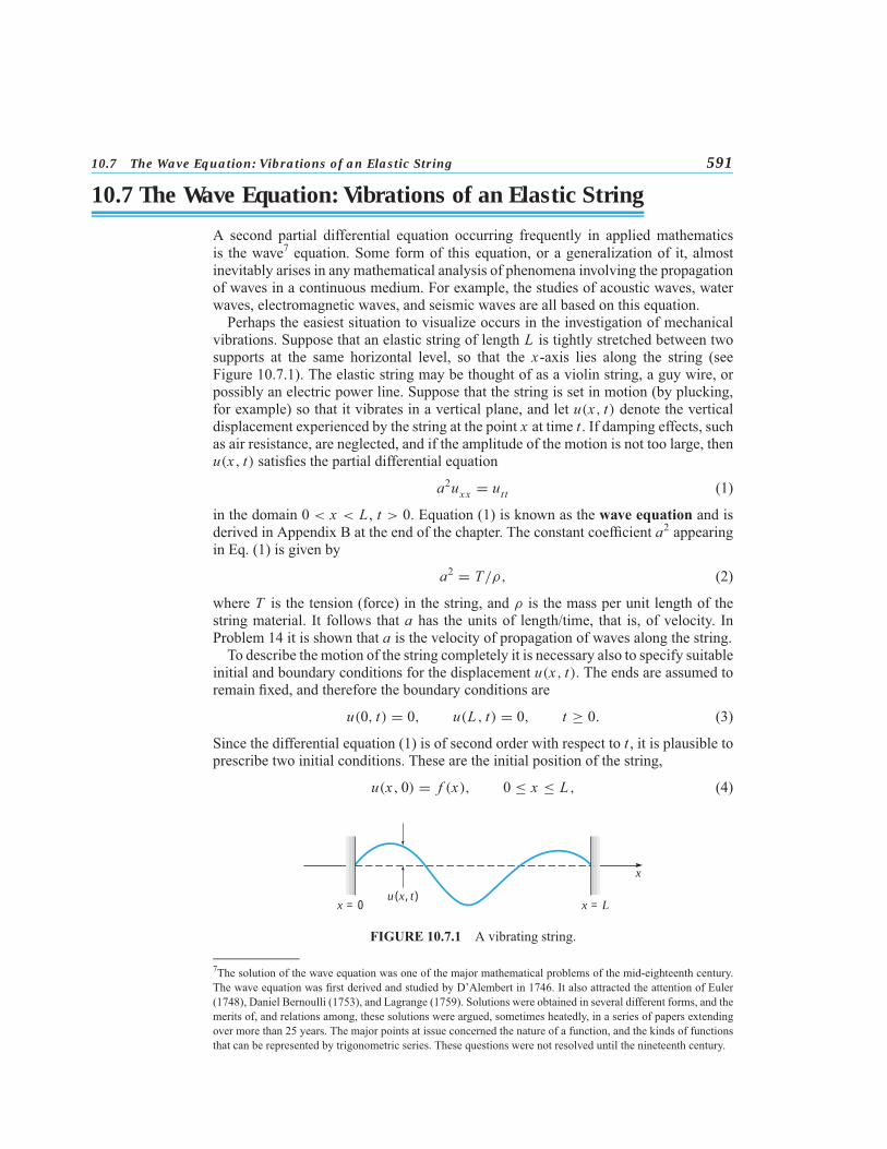
10.7 The Wave Equation: Vibrations of an Elastic String 591

10.7 The Wave Equation: Vibrations of an Elastic StringA second partial differential equation occurring frequently in applied mathematicsis the wave7 equation. Some form of this equation, or a generalization of it, almostinevitably arises in any mathematical analysis of phenomena involving the propagationof waves in a continuous medium. For example, the studies of acoustic waves, waterwaves, electromagnetic waves, and seismic waves are all based on this equation.Perhaps the easiest situation to visualize occurs in the investigation of mechanical

vibrations. Suppose that an elastic string of length L is tightly stretched between twosupports at the same horizontal level, so that the x-axis lies along the string (seeFigure 10.7.1). The elastic string may be thought of as a violin string, a guy wire, orpossibly an electric power line. Suppose that the string is set in motion (by plucking,for example) so that it vibrates in a vertical plane, and let u(x, t) denote the verticaldisplacement experienced by the string at the point x at time t . If damping effects, suchas air resistance, are neglected, and if the amplitude of the motion is not too large, thenu(x, t) satisfies the partial differential equation

a2uxx = utt (1)

in the domain 0 < x < L , t > 0. Equation (1) is known as the wave equation and isderived in Appendix B at the end of the chapter. The constant coefficient a2 appearingin Eq. (1) is given by

a2 = T/ρ, (2)

where T is the tension (force) in the string, and ρ is the mass per unit length of thestring material. It follows that a has the units of length/time, that is, of velocity. InProblem 14 it is shown that a is the velocity of propagation of waves along the string.To describe the motion of the string completely it is necessary also to specify suitable

initial and boundary conditions for the displacement u(x, t). The ends are assumed toremain fixed, and therefore the boundary conditions are

u(0, t) = 0, u(L , t) = 0, t ≥ 0. (3)

Since the differential equation (1) is of second order with respect to t , it is plausible toprescribe two initial conditions. These are the initial position of the string,

u(x, 0) = f (x), 0 ≤ x ≤ L , (4)

x

u(x, t)x = 0 x = L

FIGURE 10.7.1 A vibrating string.

7The solution of the wave equation was one of the major mathematical problems of the mid-eighteenth century.The wave equation was first derived and studied by D’Alembert in 1746. It also attracted the attention of Euler(1748), Daniel Bernoulli (1753), and Lagrange (1759). Solutions were obtained in several different forms, and themerits of, and relations among, these solutions were argued, sometimes heatedly, in a series of papers extendingover more than 25 years. The major points at issue concerned the nature of a function, and the kinds of functionsthat can be represented by trigonometric series. These questions were not resolved until the nineteenth century.


and its initial velocity,

ut(x, 0) = g(x), 0 ≤ x ≤ L , (5)

where f and g are given functions. In order for Eqs. (3), (4), and (5) to be consistentit is also necessary to require that

f (0) = f (L) = 0, g(0) = g(L) = 0. (6)

The mathematical problem then is to determine the solution of the wave equation (1)that also satisfies the boundary conditions (3) and the initial conditions (4) and (5). Likethe heat conduction problem of Sections 10.5 and 10.6, this problem is an initial valueproblem in the time variable t , and a boundary value problem in the space variable x .Alternatively, it can be considered as a boundary value problem in the semi-infinite strip0 < x < L , t > 0 of the xt-plane (see Figure 10.7.2). One condition is imposed at eachpoint on the semi-infinite sides, and two are imposed at each point on the finite base.It is important to realize that Eq. (1) governs a large number of other wave problems

besides the transverse vibrations of an elastic string. For example, it is only necessaryto interpret the function u and the constant a appropriately to have problems dealingwith water waves in an ocean, acoustic or electromagnetic waves in the atmosphere,or elastic waves in a solid body. If more than one space dimension is significant, thenEq. (1) must be slightly generalized. The two-dimensional wave equation is

a2(uxx + uyy) = utt . (7)

This equation would arise, for example, if we considered the motion of a thin elasticsheet, such as a drumhead. Similarly, in three dimensions the wave equation is

a2(uxx + uyy + uzz) = utt . (8)

In connection with the latter two equations, the boundary and initial conditions mustalso be suitably generalized.We now solve some typical boundary value problems involving the one-dimensional

wave equation.

t

x

x = L

u(0, t) = 0 u(L,t) = 0

u(x, 0) = f (x)ut(x, 0) = g(x)

a2uxx = utt

FIGURE 10.7.2 Boundary value problem for the wave equation.


Elastic String with Nonzero Initial Displacement. First suppose that the string isdisturbed from its equilibrium position, and then released at time t = 0 with zerovelocity to vibrate freely. Then the vertical displacement u(x, t) must satisfy the waveequation (1),

a2uxx = utt , 0 < x < L , t > 0;the boundary conditions (3),

u(0, t) = 0, u(L , t) = 0, t ≥ 0;and the initial conditions

u(x, 0) = f (x), ut(x, 0) = 0, 0 ≤ x ≤ L , (9)

where f is a given function describing the configuration of the string at t = 0.The method of separation of variables can be used to obtain the solution of Eqs. (1),

(3), and (9). Assuming that

u(x, t) = X (x)T (t) (10)

and substituting for u in Eq. (1), we obtain

X ′′

X= 1a2T ′′

T= −λ, (11)

where λ is a separation constant. Thus we find that X (x) and T (t) satisfy the ordinarydifferential equations

X ′′ + λX = 0, (12)T ′′ + a2λT = 0. (13)

Further, by substituting from Eq. (10) for u(x, t) in the boundary conditions (3) wefind that X (x) must satisfy the boundary conditions

X (0) = 0, X (L) = 0. (14)

Finally, by substituting from Eq. (10) into the second of the initial conditions (9), wealso find that T (t) must satisfy the initial condition

T ′(0) = 0. (15)

Our next task is to determine X (x), T (t), and λ by solving Eq. (12) subject to theboundary conditions (14) and Eq. (13) subject to the initial condition (15).The problem of solving the differential equation (12) subject to the boundary condi-

tions (14) is precisely the same problem that arose in Section 10.5 in connection withthe heat conduction equation. Thus we can use the results obtained there and at the endof Section 10.1: The problem (12) and (14) has nontrivial solutions if and only if λ isan eigenvalue,

λ = n2π2/L2, n = 1, 2, . . . , (16)

and X (x) is proportional to the corresponding eigenfunction sin(nπx/L).Using the values of λ given by Eq. (16) in Eq. (13), we obtain

T ′′ + n2π2a2

L2T = 0. (17)


Therefore

T (t) = k1 cosnπatL

+ k2 sinnπatL

, (18)

where k1 and k2 are arbitrary constants. The initial condition (15) requires that k2 = 0,so T (t) must be proportional to cos(nπat/L).Thus the functions

un(x, t) = sinnπxLcos

nπatL

, n = 1, 2, . . . , (19)

satisfy the partial differential equation (1), the boundary conditions (3), and the sec-ond initial condition (9). These functions are the fundamental solutions for the givenproblem.To satisfy the remaining (nonhomogeneous) initial condition (9) we will consider

a superposition of the fundamental solutions (19) with properly chosen coefficients.Thus we assume that u(x, t) has the form

u(x, t) =∞∑n=1

cnun(x, t) =∞∑n=1cn sin

nπxLcos

nπatL

, (20)

where the constants cn remain to be chosen. The initial condition u(x, 0) = f (x)requires that

u(x, 0) =∞∑n=1cn sin

nπxL

= f (x). (21)

Consequently, the coefficients cn must be the coefficients in the Fourier sine series ofperiod 2L for f ; hence

cn = 2L

∫ L

0f (x) sin

nπxL

dx, n = 1, 2, . . . . (22)

Thus the formal solution of the problem of Eqs. (1), (3), and (9) is given by Eq. (20)with the coefficients calculated from Eq. (22).For a fixed value of n the expression sin(nπx/L) cos(nπat/L) in Eq. (19) is periodic

in time t with the period 2L/na; it therefore represents a vibratory motion of the stringhaving this period, or having the frequency nπa/L . The quantities λa = nπa/L forn = 1, 2, . . . are the natural frequencies of the string, that is, the frequencies at whichthe stringwill freely vibrate. The factor sin(nπx/L) represents the displacement patternoccurring in the string when it is executing vibrations of the given frequency. Eachdisplacement pattern is called a natural mode of vibration and is periodic in the spacevariable x ; the spatial period 2L/n is called the wavelength of the mode of frequencynπa/L . Thus the eigenvalues n2π2/L2 of the problem (12), (14) are proportional tothe squares of the natural frequencies, and the eigenfunctions sin(nπx/L) give thenatural modes. The first three natural modes are sketched in Figure 10.7.3. The totalmotion of the string, given by the function u(x, t) of Eq. (20), is thus a combinationof the natural modes of vibration, and is also a periodic function of time with period2L/a.

10.7 The Wave Equation: Vibrations of an Elastic String 595u

x

u

x

u

xL

L L

1 11

–1–1 –1

(a) (b) (c)

FIGURE 10.7.3 First three fundamental modes of vibration of an elastic string. (a) Frequency= πa/L , wavelength= 2L; (b) frequency= 2πa/L , wavelength= L; (c) frequency= 3πa/L ,wavelength = 2L/3.

E X A M P L E

1Consider a vibrating string of length L = 30 that satisfies the wave equation

4uxx = utt , 0 < x < 30, t > 0 (23)

Assume that the ends of the string are fixed, and that the string is set in motion with noinitial velocity from the initial position

u(x, 0) = f (x) ={x/10, 0 ≤ x ≤ 10,(30− x)/20, 10 < x ≤ 30. (24)

Find the displacement u(x, t) of the string and describe its motion through one period.The solution is given by Eq. (20) with a = 2 and L = 30, that is,

u(x, t) =∞∑n=1cn sin

nπx30

cos2nπ t30

, (25)

where cn is calculated from Eq. (22). Substituting from Eq. (24) into Eq. (22), weobtain

cn = 230

∫ 10

0

x10sinnπx30

dx + 230

∫ 30

10

30− x20

sinnπx30

dx . (26)

By evaluating the integrals in Eq. (26), we find that

cn = 9n2π2

sinnπ3

, n = 1, 2, . . . . (27)

The solution (25), (27) gives the displacement of the string at any point x at any time t .The motion is periodic in time with period 30, so it is sufficient to analyze the solutionfor 0 ≤ t ≤ 30.The best way to visualize the solution is by a computer animation showing the

dynamic behavior of the vibrating string. Here we indicate the motion of the string inFigures 10.7.4, 10.7.5, and 10.7.6. Plots of u versus x for t = 0, 4, 7.5, 11, and 15are shown in Figure 10.7.4. Observe that the maximum initial displacement is positiveand occurs at x = 10, while at t = 15, a half period later, the maximum displacementis negative and occurs at x = 20. The string then retraces its motion and returns toits original configuration at t = 30. Figure 10.7.5 shows the behavior of the pointsx = 10, 15, and 20 by plots of u versus t for these fixed values of x . The plots confirmthat the motion is indeed periodic with period 30. Observe also that each interior point


on the string is motionless for one-third of each period. Figure 10.7.6 shows a three-dimensional plot of u versus both x and t , from which the overall nature of the solutionis apparent. Of course, the curves in Figures 10.7.4 and 10.7.5 lie on the surface shownin Figure 10.7.6.

x2 4 6 8 10 12 14 16 18 20 22 24 26 28 30

1

0.8

0.6

0.4

0.2

–0.2

–0.4

–0.6

–0.8

–1

u

t = 0

t = 4

t = 7.5

t = 11t = 15

FIGURE 10.7.4 Plots of u versus x for fixed values of t for the string in Example 1.

30 60

1

0.8

0.6

0.4

0.2

–0.2

–0.4

–0.6

–0.8

–1

t

u

50402010

x = 10

x = 15

x = 20

FIGURE 10.7.5 Plots of u versus t for fixed values of x for the string in Example 1.

Justification of the Solution. As in the heat conduction problem considered earlier,Eq. (20) with the coefficients cn given by Eq. (22) is only a formal solution of Eqs. (1),(3), and (9). To ascertain whether Eq. (20) actually represents the solution of the givenproblem requires some further investigation. As in the heat conduction problem, it istempting to try to show this directly by substituting Eq. (20) for u(x, t) in Eqs. (1), (3),and (9). However, on formally computing uxx , for example, we obtain

uxx(x, t) = −∞∑n=1cn

(nπL

)2sinnπxLcos

nπatL

;


30

25

20

2040

6080

15

10

5

1

–1

x

t

u

FIGURE 10.7.6 Plot of u versus x and t for the string in Example 1.

due to the presence of the n2 factor in the numerator this series may not converge. Thiswould not necessarily mean that the series (20) for u(x, t) is incorrect, but only that theseries (20) cannot be used to calculate uxx and utt . A basic difference between solutionsof the wave equation and those of the heat conduction equation is that the latter containnegative exponential terms that approach zero very rapidly with increasing n, whichensures the convergence of the series solution and its derivatives. In contrast, seriessolutions of the wave equation contain only oscillatory terms that do not decay withincreasing n.However, there is an alternative way to establish the validity of Eq. (20) indirectly. At

the same time we will gain additional information about the structure of the solution.First we will show that Eq. (20) is equivalent to

u(x, t) = 12 [h(x − at) + h(x + at)], (28)

where h is the function obtained by extending the initial data f into (−L , 0) as an oddfunction, and to other values of x as a periodic function of period 2L . That is,

h(x) ={

f (x), 0 ≤ x ≤ L ,

− f (−x), −L < x < 0; (29)

h(x + 2L) = h(x).

To establish Eq. (28) note that h has the Fourier series

h(x) =∞∑n=1cn sin

nπxL

. (30)

Then, using the trigonometric identities for the sine of a sum or difference, we obtain

h(x − at) =∞∑n=1cn

(sinnπxLcos

nπatL

− cos nπxLsinnπatL

),

h(x + at) =∞∑n=1cn

(sinnπxLcos

nπatL

+ cos nπxLsinnπatL

),


and Eq. (28) follows immediately upon adding the last two equations. From Eq. (28)we see that u(x, t) is continuous for 0 < x < L , t > 0 provided that h is continuouson the interval (−∞,∞). This requires that f be continuous on the original interval[0, L]. Similarly, u is twice continuously differentiable with respect to either variablein 0 < x < L , t > 0, provided that h is twice continuously differentiable on (−∞,∞).This requires that f ′ and f ′′ be continuous on [0, L]. Furthermore, since h′′ is the oddextension of f ′′, we must also have f ′′(0) = f ′′(L) = 0. However, since h′ is the evenextension of f ′, no further conditions are required on f ′. Provided that these conditionsare met, uxx and utt can be computed from Eq. (28), and it is an elementary exerciseto show that these derivatives satisfy the wave equation. Some of the details of theargument just indicated are given in Problems 20 and 21.If some of the continuity requirements stated in the last paragraph are not met, then u

is not differentiable at some points in the semi-infinite strip 0 < x < L , t > 0, and thusis a solution of the wave equation only in a somewhat restricted sense. An importantphysical consequence of this observation is that if there are any discontinuities presentin the initial data f , then they will be preserved in the solution u(x, t) for all time.In contrast, in heat conduction problems initial discontinuities are instantly smoothedout (Section 10.6). Suppose that the initial displacement f has a jump discontinuityat x = x0, 0 ≤ x0 ≤ L . Since h is a periodic extension of f , the same discontinuity ispresent in h(ξ) at ξ = x0 + 2nL and at ξ = −x0 + 2nL , where n is any integer. Thush(x − at) is discontinuous when x − at = x0 + 2nL , or when x − at = −x0 + 2nL .For a fixed x in [0, L] the discontinuity that was originally at x0 will reappear inh(x − at) at the times t = (x ± x0 − 2nL)/a. Similarly, h(x + at) is discontinuous atthe point x at the times t = (−x ± x0 + 2mL)/a, where m is any integer. If we referto Eq. (28), it then follows that the solution u(x, t) is also discontinuous at the givenpoint x at these times. Since the physical problem is posed for t > 0, only those valuesof m and n yielding positive values of t are of interest.

General Problem for the Elastic String. Let us modify the problem considered pre-viously by supposing that the string is set in motion from its equilibrium positionwith a given velocity. Then the vertical displacement u(x, t) must satisfy the waveequation (1),

a2uxx = utt , 0 < x < L , t > 0;the boundary conditions (3),

u(0, t) = 0, u(L , t) = 0, t ≥ 0;and the initial conditions

u(x, 0) = 0, ut(x, 0) = g(x), 0 ≤ x ≤ L , (31)

where g(x) is the initial velocity at the point x of the string.The solution of this new problem can be obtained by following the procedure de-

scribed above for the problem (1), (3), and (9). Upon separating variables, we find thatthe problem for X (x) is exactly the same as before. Thus, once again λ = n2π2/L2and X (x) is proportional to sin(nπx/L). The differential equation for T (t) is againEq. (17), but the associated initial condition is now

T (0) = 0. (32)


corresponding to the first of the initial conditions (31). The general solution of Eq. (17)is given by Eq. (18), but now the initial condition (32) requires that k1 = 0. ThereforeT (t) is now proportional to sin(nπat/L) and the fundamental solutions for the problem(1), (3), and (31) are

un(x, t) = sin nπxLsinnπatL

, n = 1, 2, 3, . . . . (33)

Each of the functions un(x, t) satisfies the wave equation (1), the boundary conditions(3), and the first of the initial conditions (31). The main consequence of using the initialconditions (31) rather than (9) is that the time-dependent factor in un(x, t) involves asine rather than a cosine.To satisfy the remaining (nonhomogeneous) initial condition we assume that u(x, t)

can be expressed as a linear combination of the fundamental solutions (33), that is,

u(x, t) =∞∑n=1knun(x, t) =

∞∑n=1kn sin

nπxLsinnπatL

. (34)

To determine the values of the coefficients kn we differentiate Eq. (34) with respectto t , set t = 0, and use the second initial condition (31); this gives the equation

ut (x, 0) =∞∑n=1

nπaLkn sin

nπxL

= g(x). (35)

Hence the quantities (nπa/L)kn are the coefficients in the Fourier sine series of period2L for g; therefore

nπaLkn = 2

L

∫ L

0g(x) sin

nπxL

dx, n = 1, 2, . . . . (36)

Thus Eq. (34), with the coefficients given by Eq. (36), constitutes a formal solutionto the problem of Eqs. (1), (3), and (31). The validity of this formal solution canbe established by arguments similar to those previously indicated for the solution ofEqs. (1), (3), and (9).Finally, we turn to the problem consisting of the wave equation (1), the boundary

conditions (3), and the general initial conditions (4), (5):

u(x, 0) = f (x), ut(x, 0) = g(x), 0 < x < L , (37)

where f (x) and g(x) are the given initial position and velocity, respectively, of thestring. Although this problem can be solved by separating variables, as in the casesdiscussed previously, it is important to note that it can also be solved simply by addingtogether the two solutions that we obtained above. To show that this is true, let v(x, t)be the solution of the problem (1), (3), and (9), and let w(x, t) be the solution of theproblem (1), (3), and (31). Thus v(x, t) is given by Eqs. (20) and (22), while w(x, t) isgiven by Eqs. (34) and (36). Now let u(x, t) = v(x, t) + w(x, t); what problem doesu(x, t) satisfy? First, observe that

a2uxx − utt = (a2vxx − vt t) + (a2wxx − wt t ) = 0+ 0 = 0, (38)

so u(x, t) satisfies the wave equation (1). Next, we have

u(0, t) = v(0, t) + w(0, t) = 0+ 0 = 0, u(L , t) = v(L , t) + w(L , t) = 0+ 0 = 0,(39)


so u(x, t) also satisfies the boundary conditions (3). Finally, we have

u(x, 0) = v(x, 0) + w(x, 0) = f (x) + 0 = f (x) (40)

and

ut(x, 0) = vt (x, 0) + wt (x, 0) = 0+ g(x) = g(x). (41)

Thus u(x, t) satisfies the general initial conditions (37).We can restate the result we have just obtained in the followingway. To solve thewave

equation with the general initial conditions (37) you can solve instead the somewhatsimpler problems with the initial conditions (9) and (31), respectively, and then addtogether the two solutions. This is another use of the principle of superposition.

PROBLEMS Consider an elastic string of length L whose ends are held fixed. The string is set in motionwith no initial velocity from an initial position u(x, 0) = f (x). In each of Problems 1 through 4carry out the following steps. Let L = 10 and a = 1 in parts (b) through (d).(a) Find the displacement u(x, t) for the given initial position f (x).(b) Plot u(x, t) versus x for 0 ≤ x ≤ 10 and for several values of t between t = 0 and t = 20.(c) Plot u(x, t) versus t for 0 ≤ t ≤ 20 and for several values of x .(d) Construct an animation of the solution in time for at least one period.(e) Describe the motion of the string in a few sentences.

� 1. f (x) ={2x/L , 0 ≤ x ≤ L/2,2(L − x)/L , L/2 < x ≤ L

� 2. f (x) =⎧⎨⎩4x/L , 0 ≤ x ≤ L/4,1, L/4 < x < 3L/4,4(L − x)/L , 3L/4 ≤ x ≤ L

� 3. f (x) = 8x(L − x)2/L3

� 4. f (x) ={1, L/2− 1 < x < L/2+ 1 (L > 2),0, otherwise

Consider an elastic string of length L whose ends are held fixed. The string is set in motion fromits equilibrium position with an initial velocity ut (x, 0) = g(x). In each of Problems 5 through8 carry out the following steps. Let L = 10 and a = 1 in parts (b) through (d).(a) Find the displacement u(x, t) for the given g(x).(b) Plot u(x, t) versus x for 0 ≤ x ≤ 10 and for several values of t between t = 0 and t = 20.(c) Plot u(x, t) versus t for 0 ≤ t ≤ 20 and for several values of x .(d) Construct an animation of the solution in time for at least one period.(e) Describe the motion of the string in a few sentences.

� 5. g(x) ={2x/L , 0 ≤ x ≤ L/2,2(L − x)/L , L/2 < x ≤ L

� 6. g(x) =⎧⎨⎩4x/L , 0 ≤ x ≤ L/4,1, L/4 < x < 3L/4,4(L − x)/L , 3L/4 ≤ x ≤ L

� 7. g(x) = 8x(L − x)2/L3

� 8. g(x) ={1, L/2− 1 < x < L/2+ 1 (L > 2),0, otherwise


9. If an elastic string is free at one end, the boundary condition to be satisfied there is thatux = 0. Find the displacement u(x, t) in an elastic string of length L , fixed at x = 0 andfree at x = L , set in motion with no initial velocity from the initial position u(x, 0) = f (x),where f is a given function.Hint: Show that the fundamental solutions for this problem, satisfying all conditions exceptthe nonhomogeneous initial condition, are

un(x, t) = sin λnx cos λnat,

where λn = (2n − 1)π/2L , n = 1, 2, . . . . Compare this problem with Problem 15 of Sec-tion 10.6; pay particular attention to the extension of the initial data out of the originalinterval [0, L].

� 10. Consider an elastic string of length L . The end x = 0 is held fixed while the end x = Lis free; thus the boundary conditions are u(0, t) = 0 and ux (L , t) = 0. The string is set inmotion with no initial velocity from the initial position u(x, 0) = f (x), where

f (x) ={1, L/2− 1 < x < L/2+ 1 (L > 2),0, otherwise.

(a) Find the displacement u(x, t).(b) With L = 10 and a = 1 plot u versus x for 0 ≤ x ≤ 10 and for several values of t . Payparticular attention to values of t between 3 and 7. Observe how the initial disturbance isreflected at each end of the string.(c) With L = 10 and a = 1 plot u versus t for several values of x .(d) Construct an animation of the solution in time for at least one period.(e) Describe the motion of the string in a few sentences.

� 11. Suppose that the string in Problem 10 is started instead from the initial position f (x) =8x(L − x)2/L3. Follow the instructions in Problem 10 for this new problem.

12. Dimensionless variables can be introduced into the wave equation a2uxx = utt in thefollowing manner. Let s = x/L and show that the wave equation becomes

a2uss = L2utt .

Then show that L/a has the dimensions of time, and thus can be used as the unit on thetime scale. Finally, let τ = at/L and show that the wave equation then reduces to

uss = uττ

.

Problems 13 and 14 indicate the form of the general solution of the wave equation and thephysical significance of the constant a.

13. Show that the wave equation

a2uxx = uttcan be reduced to the form u

ξη= 0 by change of variables ξ = x − at , η = x + at . Show

that u(x, t) can be written as

u(x, t) = φ(x − at) + ψ(x + at),where φ and ψ are arbitrary functions.

14. Plot the value of φ(x − at) for t = 0, 1/a, 2/a, and t0/a if φ(s) = sin s. Note that forany t �= 0 the graph of y = φ(x − at) is the same as that of y = φ(x) when t = 0, butdisplaced a distance at in the positive x direction. Thus a represents the velocity at whicha disturbance moves along the string. What is the interpretation of φ(x + at)?

15. A steel wire 5 ft in length is stretched by a tensile force of 50 lb. The wire has a weight perunit length of 0.026 lb/ft.(a) Find the velocity of propagation of transverse waves in the wire.


(b) Find the natural frequencies of vibration.(c) If the tension in the wire is increased, how are the natural frequencies changed? Arethe natural modes also changed?

16. A vibrating string moving in an elastic medium satisfies the equation

a2uxx − α2u = utt ,

where α2 is proportional to the coefficient of elasticity of the medium. Suppose that thestring is fixed at the ends, and is released with no initial velocity from the initial positionu(x, 0) = f (x), 0 < x < L . Find the displacement u(x, t).

17. Consider the wave equation

a2uxx = uttin an infinite one-dimensional medium subject to the initial conditions

u(x, 0) = f (x), ut (x, 0) = 0, −∞ < x < ∞.

(a) Using the form of the solution obtained in Problem 13, show that φ and ψ must satisfy

φ(x) + ψ(x) = f (x),−φ′(x) + ψ ′(x) = 0.

(b) Solve the equations of part (a) for φ and ψ , and thereby show that

u(x, t) = 12 [ f (x − at) + f (x + at)].

This form of the solution was obtained by D’Alembert in 1746.Hint: Note that the equation ψ ′(x) = φ′(x) is solved by choosing ψ(x) = φ(x) + c.(c) Let

f (x) ={2, −1 < x < 1,0, otherwise.

Show thatf (x − at) =

{2, −1+ at < x < 1+ at,0, otherwise.

Also determine f (x + at).(d) Sketch the solution found in part (b) at t = 0, t = 1/2a, t = 1/a, and t = 2/a, obtain-ing the results shown in Figure 10.7.7. Observe that an initial displacement produces twowaves moving in opposite directions away from the original location; each wave consistsof one-half of the initial displacement.

18. Consider the wave equation

a2uxx = uttin an infinite one-dimensional medium subject to the initial conditions

u(x, 0) = 0, ut (x, 0) = g(x), −∞ < x < ∞.

(a) Using the form of the solution obtained in Problem 13, show that

φ(x) + ψ(x) = 0,−aφ′(x) + aψ ′(x) = g(x).

(b) Use the first equation of part (a) to show that ψ ′(x) = −φ′(x). Then use the secondequation to show that −2aφ′(x) = g(x), and therefore that

φ(x) = − 12a

∫ x

x0

g(ξ) dξ + φ(x0),

where x0 is arbitrary. Finally, determine ψ(x).


x

u

x

x

x

u

u

u

2

1–1

1

–2–3

1

1

2

–1

–2 –1 1

1 2

2

3

–1

1

1

t = 0

t = 12a

– 32

12

32

– 12

t = 1a

t = 2a

FIGURE 10.7.7 Propagation of initial disturbance in an infinite one-dimensional medium.

(c) Show that

u(x, t) = 12a

∫ x+at

x−atg(ξ) dξ.

19. By combining the results of Problems 17 and 18 show that the solution of the problem

a2uxx = utt ,u(x, 0) = f (x), ut (x, 0) = g(x), −∞ < x < ∞

is given by

u(x, t) = 12[ f (x − at) + f (x + at)]+ 1

2a

∫ x+at

x−atg(ξ) dξ.

Problems 20 and 21 indicate how the formal solution (20), (22) of Eqs. (1), (3), and (9) can beshown to constitute the actual solution of that problem.

20. By using the trigonometric identity sin A cos B = 12 [sin(A + B) + sin(A − B)] show that

the solution (20) of the problem of Eqs. (1), (3), and (9) can be written in the form (28).21. Let h(ξ) represent the initial displacement in [0, L], extended into (−L , 0) as an odd

function and extended elsewhere as a periodic function of period 2L . Assuming thath, h′, and h′′ are all continuous, show by direct differentiation that u(x, t) as given in


Eq. (28) satisfies the wave equation (1) and also the initial conditions (9). Note also thatsince Eq. (20) clearly satisfies the boundary conditions (3), the same is true of Eq. (28).Comparing Eq. (28) with the solution of the corresponding problem for the infinite string(Problem 17), we see that they have the same form provided that the initial data for thefinite string, defined originally only on the interval 0 ≤ x ≤ L , are extended in the givenmanner over the entire x-axis. If this is done, the solution for the infinite string is alsoapplicable to the finite one.

22. The motion of a circular elastic membrane, such as a drumhead, is governed by the two-dimensional wave equation in polar coordinates

urr + (1/r)ur + (1/r2)uθθ

= a−2utt .

Assuming that u(r, θ, t) = R(r)�(θ)T (t), find ordinary differential equations satisfied byR(r), �(θ), and T (t).

23. The total energy E(t) of the vibrating string is given as a function of time by

E(t) =∫ L

0

[12ρu

2t (x, t) + 1

2Tu2x (x, t)

]dx; (i)

the first term is the kinetic energy due to the motion of the string, and the second term isthe potential energy created by the displacement of the string away from its equilibriumposition.For the displacement u(x, t) given by Eq. (20), that is, for the solution of the string

problem with zero initial velocity, show that

E(t) = π2T4L

∞∑n=1n2c2n . (ii)

Note that the right side of Eq. (ii) does not depend on t . Thus the total energy E is aconstant, and therefore is conserved during the motion of the string.Hint: Use Parseval’s equation (Problem 37 of Section 10.4 and Problem 17 of Section10.3), and recall that a2 = T/ρ.

10.8 Laplace’s EquationOne of the most important of all partial differential equations occurring in appliedmathematics is that associated with the name of Laplace8: in two dimensions

uxx + uyy = 0, (1)

and in three dimensions

uxx + uyy + uzz = 0. (2)

For example, in a two-dimensional heat conduction problem, the temperature u(x, y, t)must satisfy the differential equation

α2(uxx + uyy) = ut , (3)

8Laplace’s equation is named for Pierre-Simon de Laplace, who, beginning in 1782, studied its solutions ex-tensively while investigating the gravitational attraction of arbitrary bodies in space. However, the equation firstappeared in 1752 in a paper by Euler on hydrodynamics.

10.8 Laplace’s Equation 605

where α2 is the thermal diffusivity. If a steady-state exists, u is a function of x and yonly, and the time derivative vanishes; in this case Eq. (3) reduces to Eq. (1). Similarly,for the steady-state heat conduction problem in three dimensions, the temperature mustsatisfy the three-dimensional form of Laplace’s equation. Equations (1) and (2) alsooccur in other branches of mathematical physics. In the consideration of electrostaticfields the electric potential function in a dielectric medium containing no electriccharges must satisfy either Eq. (1) or Eq. (2), depending on the number of spacedimensions involved. Similarly, the potential function of a particle in free space actedon only by gravitational forces satisfies the same equations. Consequently, Laplace’sequation is often referred to as the potential equation. Another example arises in thestudy of the steady (time-independent), two-dimensional, inviscid, irrotational motionof an incompressible fluid, which centers about two functions, known as the velocitypotential function and the stream function, both of which satisfy Eq. (1). In elasticitythe displacements that occur when a perfectly elastic bar is twisted are described interms of the so-called warping function, which also satisfies Eq. (1).Since there is no time dependence in any of the problems mentioned previously,

there are no initial conditions to be satisfied by the solutions of Eq. (1) or (2). Theymust, however, satisfy certain boundary conditions on the bounding curve or surface ofthe region in which the differential equation is to be solved. Since Laplace’s equationis of second order, it might be plausible to expect that two boundary conditions wouldbe required to determine the solution completely. This, however, is not the case. Recallthat in the heat conduction problem for the finite bar (Sections 10.5 and 10.6) it wasnecessary to prescribe one condition at each end of the bar, that is, one conditionat each point of the boundary. If we generalize this observation to multidimensionalproblems, it is then natural to prescribe one condition on the function u at each pointon the boundary of the region in which a solution of Eq. (1) or (2) is sought. The mostcommon boundary condition occurs when the value of u is specified at each boundarypoint; in terms of the heat conduction problem this corresponds to prescribing thetemperature on the boundary. In some problems the value of the derivative, or rate ofchange, of u in the direction normal to the boundary is specified instead; the conditionon the boundary of a thermally insulated body, for example, is of this type. It is entirelypossible for more complicated boundary conditions to occur; for example, u might beprescribed on part of the boundary, and its normal derivative specified on the remainder.The problem of finding a solution of Laplace’s equation that takes on given boundaryvalues is known as a Dirichlet problem, in honor of P. G. L. Dirichlet.9 In contrast, ifthe values of the normal derivative are prescribed on the boundary, the problem is saidto be aNeumann problem, in honor of K. G. Neumann.10 The Dirichlet and Neumannproblems are also known as the first and second boundary value problems of potentialtheory, respectively.Physically, it is plausible to expect that the types of boundary conditions just men-

tioned will be sufficient to determine the solution completely. Indeed, it is possible toestablish the existence and uniqueness of the solution of Laplace’s equation under the

9Peter Gustav Dirichlet (1805–1859) was a professor at Berlin and, after the death of Gauss, at Gottingen. In1829 he gave the first set of conditions sufficient to guarantee the convergence of a Fourier series. The definitionof function usually used today in elementary calculus is essentially the one given by Dirichlet in 1837. While heis best known for his work in analysis and differential equations, Dirichlet was also one of the leading numbertheorists of the nineteenth century.10Karl GottfriedNeumann (1832–1925), professor at Leipzig, made contributions to differential equations, integralequations, and complex variables.


boundary conditions mentioned, provided the shape of the boundary and the functionsappearing in the boundary conditions satisfy certain very mild requirements. However,the proofs of these theorems, and even their accurate statement, are beyond the scopeof the present book. Our only concern will be solving some typical problems by meansof separation of variables and Fourier series.While the problems chosen as examples are capable of interesting physical interpre-

tations (in terms of electrostatic potentials or steady-state temperature distributions, forinstance), our purpose here is primarily to point out some of the features that may occurduring their mathematical solution. It is also worth noting again that more complicatedproblems can sometimes be solved by expressing the solution as the sum of solutionsof several simpler problems (see Problems 3 and 4).

Dirichlet Problem for a Rectangle. Consider the mathematical problem of findingthe function u satisfying Laplace’s equation (1),

uxx + uyy = 0,

in the rectangle 0 < x < a, 0 < y < b, and also satisfying the boundary conditions

u(x, 0) = 0, u(x, b) = 0, 0 < x < a,(4)

u(0, y) = 0, u(a, y) = f (y), 0 ≤ y ≤ b,where f is a given function on 0 ≤ y ≤ b (see Figure 10.8.1).To solve this problem we wish to construct a fundamental set of solutions satisfying

the partial differential equation and the homogeneous boundary conditions; then wewill superpose these solutions so as to satisfy the remaining boundary condition. Letus assume that

u(x, y) = X (x)Y (y) (5)

and substitute for u in Eq. (1). This yields

X ′′

X= −Y

′′

Y= λ,

where λ is the separation constant. Thus we obtain the two ordinary differentialequations

X ′′ − λX = 0, (6)Y ′′ + λY = 0. (7)

y

x

b

a

u(0, y) = 0

u(x, b) = 0

u(a, y) = f(y)

u(x,0) = 0

(a,b)

uxx + uyy = 0

FIGURE 10.8.1 Dirichlet problem for a rectangle.


Ifwe now substitute for u fromEq. (5) in each of the homogeneous boundary conditions,we find that

X (0) = 0 (8)

and

Y (0) = 0, Y (b) = 0. (9)

We will first determine the solution of the differential equation (7) subject to theboundary conditions (9). However, this problem is essentially identical to one encoun-tered previously in Sections 10.1, 10.5, and 10.7. We conclude that there are nontrivialsolutions if and only if λ is an eigenvalue, namely,

λ = (nπ/b)2, n = 1, 2, . . . ; (10)

and Y (y) is proportional to the corresponding eigenfunction sin(nπy/b). Next, wesubstitute from Eq. (10) for λ in Eq. (6), and solve this equation subject to the boundarycondition (8). It is convenient to write the general solution of Eq. (6) as

X (x) = k1 cosh(nπx/b) + k2 sinh(nπx/b), (11)

and the boundary condition (8) then requires that k1 = 0. Therefore X (x) must beproportional to sinh(nπx/b). Thus we obtain the fundamental solutions

un(x, y) = sinhnπxbsinnπyb

, n = 1, 2, . . . . (12)

These functions satisfy the differential equation (1) and all the homogeneous boundaryconditions for each value of n.To satisfy the remaining nonhomogeneous boundary condition at x = a we assume,

as usual, that we can represent the solution u(x, y) in the form

u(x, y) =∞∑n=1cnun(x, y) =

∞∑n=1cn sinh

nπxbsinnπyb

. (13)

The coefficients cn are determined by the boundary condition

u(a, y) =∞∑n=1cn sinh

nπabsinnπyb

= f (y). (14)

Therefore the quantities cn sinh(nπa/b) must be the coefficients in the Fourier sineseries of period 2b for f and are given by

cn sinhnπab

= 2b

∫ b

0f (y) sin

nπybdy. (15)

Thus the solution of the partial differential equation (1) satisfying the boundary condi-tions (4) is given by Eq. (13) with the coefficients cn computed from Eq. (15).From Eqs. (13) and (15) we see that the solution contains the factor

sinh(nπx/b)/ sinh(nπa/b). To estimate this quantity for large n we can use theapproximation sinh ξ ∼= eξ /2, and thereby obtain

sinh(nπx/b)sinh(nπa/b)

∼=12 exp(nπx/b)12 exp(nπa/b)

= exp[−nπ(a − x)/b].

Thus this factor has the character of a negative exponential; consequently, the series(13) converges quite rapidly unless a − x is very small.


E X A M P L E

1To illustrate these results, let a = 3, b = 2, and

f (y) ={y, 0 ≤ y ≤ 1,2− y, 1 ≤ y ≤ 2. (16)

By evaluating cn from Eq. (15) we find that

cn = 8 sin(nπ/2)n2π2 sinh(3nπ/2)

. (17)

Then u(x, y) is given by Eq. (13). Keeping 20 terms in the series we can plot u versusx and y, as shown in Figure 10.8.2. Alternatively, one can construct a contour plotshowing level curves of u(x, y); Figure 10.8.3 is such a plot, with an increment of 0.1between adjacent curves.

3y x

u

21

0.21

2 0.4

0.6

0.8

1.0

FIGURE 10.8.2 Plot of u versus x and y for Example 1.

1

x

2

y

u = 0

u = 0

u = 0u = 0.9u = 0.7u = 0.5

u = 0.4u = 0.2

u = 0.6u = 0.8

u = 0.3u = 0.1

321

FIGURE 10.8.3 Level curves of u(x, y) for Example 1.


Dirichlet Problem for a Circle. Consider the problem of solving Laplace’s equationin a circular region r < a subject to the boundary condition

u(a, θ) = f (θ), (18)

where f is a given function on 0 ≤ θ < 2π (see Figure 10.8.4). In polar coordinatesLaplace’s equation takes the form

urr + 1rur + 1

r2u

θθ= 0. (19)

To complete the statement of the problem we note that for u(r, θ) to be single-valued,it is necessary that u be periodic in θ with period 2π . Moreover, we state explicitly thatu(r, θ) must be bounded for r ≤ a, since this will become important later.To apply the method of separation of variables to this problem we assume that

u(r, θ) = R(r)�(θ), (20)

and substitute for u in the differential equation (19). This yields

R′′� + 1rR′� + 1

r2R�′′ = 0,

or

r2R′′

R+ r R

′

R= −�′′

�= λ, (21)

where λ is the separation constant. Thus we obtain the two ordinary differentialequations

r2R′′ + r R′ − λR = 0, (22)�′′ + λ� = 0. (23)

In this problem there are no homogeneous boundary conditions; recall, however, thatsolutions must be bounded and also periodic in θ with period 2π . It is possible to show(Problem 9) that the periodicity condition requires that λmust be real. We will considerin turn the cases in which λ is negative, zero, and positive.

y

x

a

θ

u(a, ) = f ( )θ θ

urr + ur + u = 01r

1r2 θθ

FIGURE 10.8.4 Dirichlet problem for a circle.


If λ < 0, let λ = −μ2, where μ > 0. Then Eq. (23) becomes �′′ − μ2� = 0, andconsequently

�(θ) = c1eμθ + c2e−μθ . (24)

Thus �(θ) can be periodic only if c1 = c2 = 0, and we conclude that λ cannot benegative.If λ = 0, then Eq. (23) becomes �′′ = 0, and thus

�(θ) = c1 + c2θ. (25)

For �(θ) to be periodic we must have c2 = 0, so that �(θ) is a constant. Further, forλ = 0, Eq. (22) becomes

r2R′′ + r R′ = 0. (26)

This equation is of the Euler type, and has the solution

R(r) = k1 + k2 ln r. (27)

The logarithmic termcannot be accepted if u(r, θ) is to remain bounded as r → 0; hencek2 = 0. Thus, corresponding to λ = 0, we conclude that u(r, θ) must be a constant,that is, proportional to the solution

u0(r, θ) = 1. (28)

Finally, if λ > 0, we let λ = μ2 where μ > 0. Then Eqs. (22) and (23) become

r2R′′ + r R′ − μ2R = 0 (29)

and

�′′ + μ2� = 0, (30)

respectively. Equation (29) is an Euler equation and has the solution

R(r) = k1rμ + k2r−μ, (31)

while Eq. (30) has the solution

�(θ) = c1 sinμθ + c2 cosμθ. (32)

In order that � be periodic with period 2π it is necessary that μ be a positive integern. With μ = n it follows that the solution r−μ in Eq. (31) must be discarded since itbecomes unbounded as r → 0. Consequently, k2 = 0 and the appropriate solutions ofEq. (19) are

un(r, θ) = rn cos nθ, vn(r, θ) = rn sin nθ, n = 1, 2, . . . . (33)

These functions, together with u0(r, θ) = 1, form a set of fundamental solutions forthe present problem.In the usual way we now assume that u can be expressed as a linear combination of

the fundamental solutions; that is,

u(r, θ) = c02

+∞∑n=1rn(cn cos nθ + kn sin nθ). (34)


The boundary condition (18) then requires that

u(a, θ) = c02

+∞∑n=1an(cn cos nθ + kn sin nθ) = f (θ) (35)

for 0 ≤ θ < 2π . The function f may be extended outside this interval so that it isperiodic with period 2π , and therefore has a Fourier series of the form (35). Sincethe extended function has period 2π , we may compute its Fourier coefficients byintegrating over any period of the function. In particular, it is convenient to use theoriginal interval (0, 2π); then

ancn = 1π

∫ 2π

0f (θ) cos nθ dθ, n = 0, 1, 2, . . . ; (36)

ankn = 1π

∫ 2π

0f (θ) sin nθ dθ, n = 1, 2, . . . . (37)

With this choice of the coefficients, Eq. (34) represents the solution of the boundaryvalue problem of Eqs. (18) and (19). Note that in this problem we needed both sineand cosine terms in the solution. This is because the boundary data were given on0 ≤ θ < 2π and have period 2π . As a consequence, the full Fourier series is required,rather than sine or cosine terms alone.

PROBLEMS� 1. (a) Find the solution u(x, y) of Laplace’s equation in the rectangle 0 < x < a, 0 < y < b,

also satisfying the boundary conditions

u(0, y) = 0, u(a, y) = 0, 0 < y < b,u(x, 0) = 0, u(x, b) = g(x), 0 ≤ x ≤ a.

(b) Find the solution if

g(x) ={x, 0 ≤ x ≤ a/2,a − x, a/2 ≤ x ≤ a.

(c) For a = 3 and b = 1 plot u versus x for several values of y and also plot u versus y forseveral values of x .(d) Plot u versus both x and y in three dimensions. Also draw a contour plot showingseveral level curves of u(x, y) in the xy-plane.

2. Find the solution u(x, y) of Laplace’s equation in the rectangle 0 < x < a, 0 < y < b, alsosatisfying the boundary conditions

u(0, y) = 0, u(a, y) = 0, 0 < y < b,u(x, 0) = h(x), u(x, b) = 0, 0 ≤ x ≤ a.

� 3. (a) Find the solution u(x, y) of Laplace’s equation in the rectangle 0 < x < a, 0 < y < b,also satisfying the boundary conditions

u(0, y) = 0, u(a, y) = f (y), 0 < y < b,u(x, 0) = h(x), u(x, b) = 0, 0 ≤ x ≤ a.

Hint: Consider the possibility of adding the solutions of two problems, one with homo-geneous boundary conditions except for u(a, y) = f (y), and the other with homogeneousboundary conditions except for u(x, 0) = h(x).(b) Find the solution if h(x) = (x/a)2 and f (y) = 1− (y/b).(c) Let a = 2 and b = 2. Plot the solution in several ways: u versus x , u versus y, u versusboth x and y, and a contour plot.


4. Show how to find the solution u(x, y) of Laplace’s equation in the rectangle 0 < x < a,0 < y < b, also satisfying the boundary conditions

u(0, y) = k(y), u(a, y) = f (y), 0 < y < b,u(x, 0) = h(x), u(x, b) = g(x), 0 ≤ x ≤ a.

Hint: See Problem 3.5. Find the solution u(r, θ) of Laplace’s equation

urr + (1/r)ur + (1/r2)uθθ

= 0

outside the circle r = a, also satisfying the boundary conditionu(a, θ) = f (θ), 0 ≤ θ < 2π,

on the circle. Assume that u(r, θ) is single-valued and bounded for r > a.� 6. (a) Find the solution u(r, θ) of Laplace’s equation in the semicircular region r < a,

0 < θ < π , also satisfying the boundary conditions

u(r, 0) = 0, u(r, π) = 0, 0 ≤ r < a,u(a, θ) = f (θ), 0 ≤ θ ≤ π.

Assume that u is single-valued and bounded in the given region.(b) Find the solution if f (θ) = θ(π − θ).(c) Let a = 2 and plot the solution in several ways: u versus r , u versus θ , u versus bothr and θ , and a contour plot.

7. Find the solution u(r, θ) of Laplace’s equation in the circular sector 0 < r < a, 0 < θ < α,also satisfying the boundary conditions

u(r, 0) = 0, u(r, α) = 0, 0 ≤ r < a,u(a, θ) = f (θ), 0 ≤ θ ≤ α.

Assume that u is single-valued and bounded in the sector.� 8. (a) Find the solution u(x, y) of Laplace’s equation in the semi-infinite strip 0 < x < a,

y > 0, also satisfying the boundary conditions

u(0, y) = 0, u(a, y) = 0, y > 0,u(x, 0) = f (x), 0 ≤ x ≤ a

and the additional condition that u(x, y) → 0 as y → ∞.(b) Find the solution if f (x) = x(a − x).(c) Let a = 5. Find the smallest value of y0 for which u(x, y) ≤ 0.1 for all y ≥ y0.

9. Show that Eq. (23) has periodic solutions only if λ is real.Hint: Let λ = −μ2 where μ = ν + iσ with ν and σ real.

10. Consider the problem of finding a solution u(x, y) of Laplace’s equation in the rectangle0 < x < a, 0 < y < b, also satisfying the boundary conditions

ux (0, y) = 0, ux (a, y) = f (y), 0 < y < b,uy(x, 0) = 0, uy(x, b) = 0, 0 ≤ x ≤ a.

This is an example of a Neumann problem.(a) Show that Laplace’s equation and the homogeneous boundary conditions determinethe fundamental set of solutions

u0(x, y) = c0,un(x, y) = cn cosh(nπx/b) cos(nπy/b), n = 1, 2, 3, . . . .

(b) By superposing the fundamental solutions of part (a), formally determine a function ualso satisfying the nonhomogeneous boundary condition ux (a, y) = f (y). Note that whenux (a, y) is calculated, the constant term in u(x, y) is eliminated, and there is no condition


from which to determine c0. Furthermore, it must be possible to express f by means of aFourier cosine series of period 2b, which does not have a constant term. This means that∫ b

0f (y) dy = 0

is a necessary condition for the given problem to be solvable. Finally, note that c0 remainsarbitrary, and hence the solution is determined only up to this additive constant. This is aproperty of all Neumann problems.

11. Find a solution u(r, θ) of Laplace’s equation inside the circle r = a, also satisfying theboundary condition on the circle

ur (a, θ) = g(θ), 0 ≤ θ < 2π.

Note that this is a Neumann problem, and that its solution is determined only up to anarbitrary additive constant. State a necessary condition on g(θ) for this problem to besolvable by the method of separation of variables (see Problem 10).


u(0, y) = 0, u(a, y) = 0, 0 < y < b,uy(x, 0) = 0, u(x, b) = g(x), 0 ≤ x ≤ a.

Note that this is neither a Dirichlet nor a Neumann problem, but a mixed problem in whichu is prescribed on part of the boundary and its normal derivative on the rest.(b) Find the solution if

g(x) ={x, 0 ≤ x ≤ a/2,a − x, a/2 ≤ x ≤ a.

(c) Let a = 3 and b = 1. By drawing suitable plots compare this solution with the solutionof Problem 1.


u(0, y) = 0, u(a, y) = f (y), 0 < y < b,u(x, 0) = 0, uy(x, b) = 0, 0 ≤ x ≤ a.

Hint: Eventually it will be necessary to expand f (y) in a series making use of the functionssin(πy/2b), sin(3πy/2b), sin(5πy/2b), . . . (see Problem 39 of Section 10.4).(b) Find the solution if f (y) = y(2b − y).(c) Let a = 3 and b = 2; plot the solution in several ways.


ux (0, y) = 0, ux (a, y) = 0, 0 < y < b,u(x, 0) = 0, u(x, b) = g(x), 0 ≤ x ≤ a.

(b) Find the solution if g(x) = 1+ x2(x − a)2.(c) Let a = 3 and b = 2; plot the solution in several ways.

15. By writing Laplace’s equation in cylindrical coordinates r , θ , and z and then assuming thatthe solution is axially symmetric (no dependence on θ ), we obtain the equation

urr + (1/r)ur + uzz = 0.Assuming that u(r, z) = R(r)Z(z), show that R and Z satisfy the equations

r R′′ + R′ + λ2r R = 0, Z ′′ − λ2Z = 0.

The equation for R is Bessel’s equation of order zero with independent variable λr .


A P P E N D I X

ADerivation of the Heat Conduction Equation. In this section we derive the differ-ential equation that, to a first approximation at least, governs the conduction of heatin solids. It is important to understand that the mathematical analysis of a physicalsituation or process such as this ultimately rests on a foundation of empirical knowl-edge of the phenomenon involved. The mathematician must have a place to start, soto speak, and this place is furnished by experience. Consider a uniform rod insulatedon the lateral surfaces so that heat can flow only in the axial direction. It has beendemonstrated many times that if two parallel cross sections of the same area A anddifferent temperatures T1 and T2, respectively, are separated by a small distance d,an amount of heat per unit time will pass from the warmer section to the cooler one.Moreover, this amount of heat is proportional to the area A, the temperature difference| T2 − T1|, and inversely proportional to the separation distance d. Thus

Amount of heat per unit time = κA| T2 − T1|/d, (1)

where the positive proportionality factor κ is called the thermal conductivity anddepends primarily on the material11 of the rod. The relation (1) is often called Fourier’slaw of heat conduction. We repeat that Eq. (1) is an empirical, not a theoretical, resultand that it can be, and has often been, verified by careful experiment. It is the basis ofthe mathematical theory of heat conduction.Now consider a straight rod of uniform cross section and homogeneous material,

oriented so that the x-axis lies along the axis of the rod (see Figure 10.A.1). Let x = 0and x = L designate the ends of the bar.

x = x0 x = x0 + Δx

H = – Auxκ H = Auxκ

x

FIGURE 10.A.1 Conduction of heat in an element of a rod.

We will assume that the sides of the bar are perfectly insulated so that there is nopassage of heat through them. We will also assume that the temperature u dependsonly on the axial position x and the time t , and not on the lateral coordinates y and z.In other words, we assume that the temperature remains constant on any cross sectionof the bar. This assumption is usually satisfactory when the lateral dimensions of therod are small compared to its length.The differential equation governing the temperature in the bar is an expression of a

fundamental physical balance; the rate at which heat flows into any portion of the baris equal to the rate at which heat is absorbed in that portion of the bar. The terms in theequation are called the flux (flow) term and the absorption term, respectively.We will first calculate the flux term. Consider an element of the bar lying between

the cross sections x = x0 and x = x0 + �x , where x0 is arbitrary and�x is small. The

11Actually, κ also depends on the temperature, but if the temperature range is not too great, it is satisfactory toassume that κ is independent of temperature.

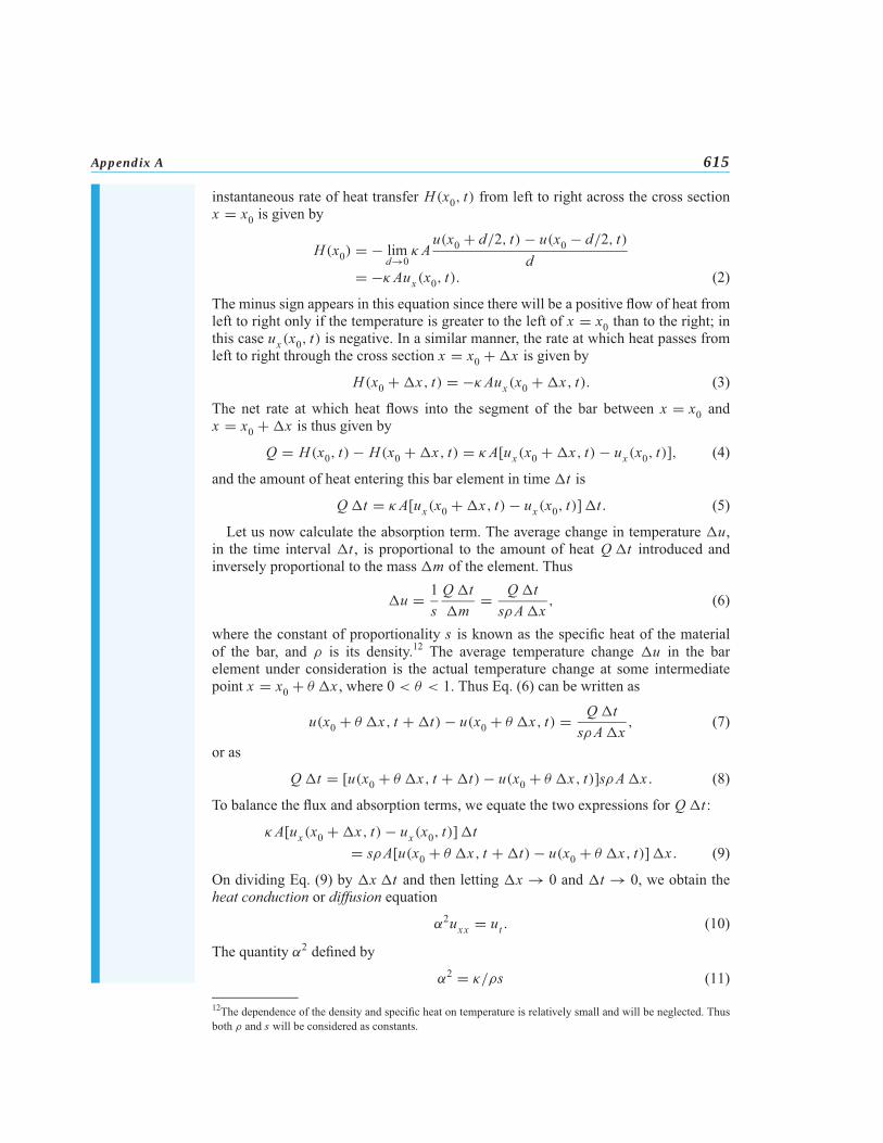
Appendix A 615

instantaneous rate of heat transfer H(x0, t) from left to right across the cross sectionx = x0 is given by

H(x0) = − limd→0

κAu(x0 + d/2, t) − u(x0 − d/2, t)

d= −κAux(x0, t). (2)

The minus sign appears in this equation since there will be a positive flow of heat fromleft to right only if the temperature is greater to the left of x = x0 than to the right; inthis case ux(x0, t) is negative. In a similar manner, the rate at which heat passes fromleft to right through the cross section x = x0 + �x is given by

H(x0 + �x, t) = −κAux(x0 + �x, t). (3)

The net rate at which heat flows into the segment of the bar between x = x0 andx = x0 + �x is thus given by

Q = H(x0, t) − H(x0 + �x, t) = κA[ux(x0 + �x, t) − ux(x0, t)], (4)

and the amount of heat entering this bar element in time �t is

Q�t = κA[ux(x0 + �x, t) − ux(x0, t)]�t. (5)

Let us now calculate the absorption term. The average change in temperature �u,in the time interval �t , is proportional to the amount of heat Q�t introduced andinversely proportional to the mass �m of the element. Thus

�u = 1sQ�t�m

= Q�tsρA�x

, (6)

where the constant of proportionality s is known as the specific heat of the materialof the bar, and ρ is its density.12 The average temperature change �u in the barelement under consideration is the actual temperature change at some intermediatepoint x = x0 + θ �x , where 0 < θ < 1. Thus Eq. (6) can be written as

u(x0 + θ �x, t + �t) − u(x0 + θ �x, t) = Q�tsρA�x

, (7)

or as

Q�t = [u(x0 + θ �x, t + �t) − u(x0 + θ �x, t)]sρA�x . (8)

To balance the flux and absorption terms, we equate the two expressions for Q�t :

κA[ux(x0 + �x, t) − ux(x0, t)]�t= sρA[u(x0 + θ �x, t + �t) − u(x0 + θ �x, t)]�x . (9)

On dividing Eq. (9) by �x �t and then letting �x → 0 and �t → 0, we obtain theheat conduction or diffusion equation

α2uxx = ut . (10)

The quantity α2 defined by

α2 = κ/ρs (11)

12The dependence of the density and specific heat on temperature is relatively small and will be neglected. Thusboth ρ and s will be considered as constants.


is called the thermal diffusivity, and is a parameter depending only on the material ofthe bar. The units ofα2 are (length)2/time. Typical values ofα2 are given inTable 10.5.1.Several relatively simple conditions may be imposed at the ends of the bar. For

example, the temperature at an end may be maintained at some constant value T . Thismight be accomplished by placing the end of the bar in thermal contact with somereservoir of sufficient size so that any heat that may flow between the bar and reservoirdoes not appreciably alter the temperature of the reservoir. At an end where this is donethe boundary condition is

u = T . (12)

Another simple boundary condition occurs if the end is insulated so that no heatpasses through it. Recalling the expression (2) for the amount of heat crossing anycross section of the bar, we conclude that the condition of insulation is that thisquantity vanish. Thus

ux = 0 (13)

is the boundary condition at an insulated end.A more general type of boundary condition occurs if the rate of flow of heat through

an end of the bar is proportional to the temperature there. Let us consider the end x = 0,where the rate of flow of heat from left to right is given by −κAux(0, t); see Eq. (2).Hence the rate of heat flow out of the bar (from right to left) at x = 0 is κAux(0, t).If this quantity is proportional to the temperature u(0, t), then we obtain the boundarycondition

ux(0, t) − h1u(0, t) = 0, t > 0, (14)

where h1 is a nonnegative constant of proportionality. Note that h1 = 0 corresponds toan insulated end, while h1 → ∞ corresponds to an end held at zero temperature.If heat flow is taking place at the right end of the bar (x = L), then in a similar way

we obtain the boundary condition

ux(L , t) + h2u(L , t) = 0, t > 0, (15)

where again h2 is a nonnegative constant of proportionality.Finally, to determine completely the flow of heat in the bar it is necessary to state

the temperature distribution at one fixed instant, usually taken as the initial time t = 0.This initial condition is of the form

u(x, 0) = f (x), 0 ≤ x ≤ L . (16)

The problem then is to determine the solution of the differential equation (10) subjectto one of the boundary conditions (12) to (15) at each end, and to the initial condition(16) at t = 0.Several generalizations of the heat equation (10) also occur in practice. First, the

bar material may be nonuniform and the cross section may not be constant along thelength of the bar. In this case, the parameters κ , ρ, s, and A may depend on the axialvariable x . Going back to Eq. (2) we see that the rate of heat transfer from left to rightacross the cross section at x = x0 is now given by

H(x0, t) = −κ(x0)A(x0)ux(x0, t) (17)

Appendix B 617

with a similar expression for H(x0 + �x, t). Ifwe introduce these quantities intoEq. (4)and eventually into Eq. (9), and proceed as before, we obtain the partial differentialequation

(κAux)x = sρAut . (18)

We will usually write Eq. (18) in the form

r(x)ut = [p(x)ux ]x , (19)

where p(x) = κ(x)A(x) and r(x) = s(x)ρ(x)A(x). Note that both these quantities areintrinsically positive.A second generalization occurs if there are other ways in which heat enters or leaves

the bar. Suppose that there is a source that adds heat to the bar at a rate G(x, t, u)per unit time per unit length, where G(x, t, u) > 0. In this case we must add the termG(x, t, u)�x �t to the left side of Eq. (9), and this leads to the differential equation

r(x)ut = [p(x)ux ]x + G(x, t, u). (20)

If G(x, t, u) < 0, then we speak of a sink that removes heat from the bar at the rateG(x, t, u) per unit time per unit length. To make the problem tractable we must restrictthe form of the function G. In particular, we assume that G is linear in u and that thecoefficient of u does not depend on t . Thus we write

G(x, t, u) = F(x, t) − q(x)u. (21)

The minus sign in Eq. (21) has been introduced so that certain equations that appearlater will have their customary forms. Substituting from Eq. (21) into Eq. (20), weobtain

r(x)ut = [p(x)ux ]x − q(x)u + F(x, t). (22)

This equation is sometimes called the generalized heat conduction equation. Boundaryvalue problems for Eq. (22) will be discussed to some extent in Chapter 11.Finally, if instead of a one-dimensional bar, we consider a body with more than one

significant space dimension, then the temperature is a function of two or three spacecoordinates rather than of x alone. Considerations similar to those leading to Eq. (10)can be employed to derive the heat conduction equation in two dimensions,

α2(uxx + uyy) = ut , (23)

or in three dimensions,

α2(uxx + uyy + uzz) = ut . (24)

The boundary conditions corresponding to Eqs. (12) and (13) for multidimensionalproblems correspond to a prescribed temperature distribution on the boundary, or to aninsulated boundary. Similarly, the initial temperature distribution will in general be afunction of x and y for Eq. (23), and a function of x , y, and z for Eq. (24).

A P P E N D I X

BDerivation of the Wave Equation. In this appendix we derive the wave equation inone space dimension as it applies to the transverse vibrations of an elastic string, orcable; the elastic string may be thought of as a violin string, a guy wire, or possibly anelectric power line. The same equation, however,with the variables properly interpreted,occurs in many other wave problems having only one significant space variable.


Consider a perfectly flexible elastic string stretched tightly between supports fixedat the same horizontal level (see Figure 10.B.1a). Let the x-axis lie along the stringwith the endpoints located at x = 0 and x = L . If the string is set in motion at someinitial time t = 0 (by plucking, for example) and is thereafter left undisturbed, it willvibrate freely in a vertical plane provided that damping effects, such as air resistance,are neglected. To determine the differential equation governing this motion we willconsider the forces acting on a small element of the string of length �x lying betweenthe points x and x + �x (see Figure 10.B.1b). We assume that the motion of the stringis small, and as a consequence, each point on the string moves solely in a verticalline. We denote by u(x, t) the vertical displacement of the point x at the time t . Letthe tension in the string, which always acts in the tangential direction, be denoted byT (x, t), and let ρ denote the mass per unit length of the string.Newton’s law, as it applies to the element�x of the string, states that the net external

force, due to the tension at the ends of the element, must be equal to the product of themass of the element and the acceleration of its mass center. Since there is no horizontalacceleration, the horizontal components must satisfy

T (x + �x, t) cos(θ + �θ) − T (x, t) cos θ = 0. (1)

If we denote the horizontal component of the tension (see Figure 10.B.1c) by H , thenEq. (1) states that H is independent of x .On the other hand, the vertical components satisfy

T (x + �x, t) sin(θ + �θ) − T (x, t) sin θ = ρ �x utt(x, t), (2)

where x is the coordinate of the center of mass of the element of the string underconsideration. Clearly, x lies in the interval x < x < x + �x . The weight of the string,

u

x

TT

θθ

T

x ⎯x x + Δx

(a)

(b) (c)

T (x + Δx, t)θ θ+ Δ

V = T sinθ

H = T cos θT(x, t)

x = 0 x = L

FIGURE 10.B.1 (a) An elastic string under tension. (b) An element of the displaced string.(c) Resolution of the tension T into components.

Appendix B 619

which acts vertically downward, is assumed to be negligible, and has been neglectedin Eq. (2).If the vertical component of T is denoted by V , then Eq. (2) can be written as

V (x + �x, t) − V (x, t)�x

= ρutt(x, t).

Passing to the limit as �x → 0 gives

Vx(x, t) = ρutt(x, t). (3)

To express Eq. (3) entirely in terms of u we note that

V (x, t) = H(t) tan θ = H(t)ux(x, t).

Hence Eq. (3) becomes(Hux)x = ρutt ,

or, since H is independent of x ,Huxx = ρutt . (4)

For small motions of the string it is permissible to replace H = T cos θ by T . ThenEq. (4) takes its customary form

a2uxx = utt , (5)

wherea2 = T/ρ. (6)

We will assume further that a2 is a constant, although this is not required in ourderivation, even for small motions. Equation (5) is called the wave equation for onespace dimension. Since T has the dimension of force, and ρ that of mass/length, itfollows that the constant a has the dimension of velocity. It is possible to identify a asthe velocity with which a small disturbance (wave) moves along the string. Accordingto Eq. (6) the wave velocity a varies directly with the tension in the string, but inverselywith the density of the string material. These facts are in agreement with experience.As in the case of the heat conduction equation, there are various generalizations of

the wave equation (5). One important equation is known as the telegraph equation andhas the form

utt + cut + ku = a2uxx + F(x, t), (7)

where c and k are nonnegative constants. The terms cut , ku, and F(x, t) arise from aviscous damping force, an elastic restoring force, and an external force, respectively.Note the similarity of Eq. (7), except for the term a2uxx , with the equation for thespring–mass system derived in Section 3.8; the additional term a2uxx arises from aconsideration of internal elastic forces.For a vibrating system with more than one significant space coordinate, it may be

necessary to consider the wave equation in two dimensions,

a2(uxx + uyy) = utt , (8)

or in three dimensions,

a2(uxx + uyy + uzz) = utt . (9)


REFERENCES The following books contain additional information on Fourier series:Buck, R. C., and Buck, E. F., Advanced Calculus (3rd ed.) (New York: McGraw-Hill, 1978).Carslaw, H. S., Introduction to the Theory of Fourier’s Series and Integrals (3rd ed.) (Cambridge:Cambridge University Press, 1930; New York: Dover, 1952).

Courant, R., and John, F., Introduction to Calculus and Analysis (New York: Wiley-Interscience,1965; reprinted by Springer-Verlag, New York, 1989).

Kaplan, W., Advanced Calculus (4th ed.) (Reading, MA: Addison-Wesley, 1991).A brief biography of Fourier and an annotated copy of his 1807 paper are contained in:

Grattan-Guinness, I., Joseph Fourier 1768–1830 (Cambridge, MA: MIT Press, 1973).Useful references on partial differential equations and the method of separation of variables include the

following:Churchill, R. V., and Brown, J. W., Fourier Series and Boundary Value Problems (5th ed.) (NewYork: McGraw-Hill, 1993).

Haberman, R., Elementary Applied Partial Differential Equations (3rd ed.) (Englewood Cliffs, NJ:Prentice Hall, 1998).

Pinsky, M. A., Partial Differential Equations and Boundary Value Problems with Applications (3rded.) (Boston: WCB/McGraw-Hill, 1998).

Powers, D. L., Boundary Value Problems (4th ed.) (San Diego: Academic Press, 1999).Strauss, W. A., Partial Differential Equations, an Introduction (New York: Wiley, 1992).Weinberger, H. F., A First Course in Partial Differential Equations (New York: Wiley, 1965; NewYork: Dover, 1995).

C H A P T E R

11

Boundary ValueProblems andSturm–LiouvilleTheoryAs a result of separating variables in a partial differential equation in Chapter 10 werepeatedly encountered the differential equation

X ′′ + λX = 0, 0 < x < L

with the boundary conditions

X (0) = 0, X (L) = 0.

This boundary value problem is the prototype of a large class of problems that are impor-tant in applied mathematics. These problems are known as Sturm–Liouville boundaryvalue problems. In this chapter we discuss the major properties of Sturm–Liouvilleproblems and their solutions; in the process we are able to generalize somewhat themethod of separation of variables for partial differential equations.

11.1 The Occurrence of Two-Point Boundary Value ProblemsIn Chapter 10 we described the method of separation of variables as a means of solvingcertain problems involving partial differential equations. The heat conduction problemconsisting of the partial differential equation

α2uxx = ut , 0 < x < L , t > 0 (1)

621

10 partial differential equations and fourier seriesfaculty.ccp.edu/faculty/akitover/272/chapter...

Documents