10. Appendix. The code RADAU5

Based on the 3-stage Radau IIA method, given in Table 2.2, a FORTRANprogram has been presented in Hairer & Wanner (1988). We have modified itslightly, so that it is also applicable to differential-algebraic systems of index 1,2, and 3. This program can be applied to initial value problems of the form

By' = f(x, y), (10.1)

where B is a constant square matrix. Of course, B may be singular.In this section we give the documentation of this code, and we explain at an

example how it can be used. Readers who wish to experiment with RADAU5 areinvited to write to one of the authors. You will receive the latest version of thecode.Address: Section de Mathematiques, Case postale 240, CH-1211 Geneve 24,

SwitzerlandE-mail: HAIRER@CGEUGE51.BITNET

Driver example for the pendulum

The use of a code can best be seen at an example. We therefore considerthe index 2 problem (1.20) on the interval [0,10]. The subroutines FPEND andBPEND specify the right-hand side of the differential-algebraic system (10.1) andthe matrix B, repectively. Further a subroutine SOLOUT is provided, which isused to print the solution at equidistant points. This subroutine need not bespecified if the solution is needed only at the endpoint of integration. It shouldbe mentioned that the function CONTR5 allows to compute an approximation tothe solution also between two grid-points. It is especially helpful for graphics.

For problems of index 2 or index 3 it may be important to scale the differential-algebraic variables (see formula (8.13)). For the index 2 problem (1.10) this isdone by choosing IWORK(5) and IWORK(6) equal to the dimensions of the vectorsy and z, respectively. The y- and z-components must appear in this order in thearray Y. For the index 3 system (1.17) the parameters IWORK(5), IWORK(6) andIWORK(7) have to be equal to the dimensions of y, z, and u, respectively. By de-creasing the safety factor for the convergence test of Newton's method (WORK(4))and increasing the maximum number of Newton iterations (IWORK(3)) the code,can be made safer.

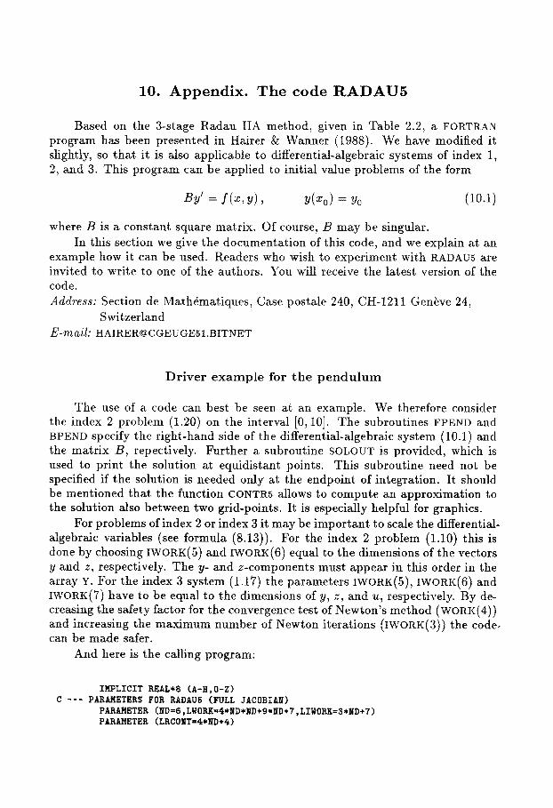
And here is the calling program:

IMPLICIT REAL*8 (A-H,O-Z)C --- PARAMETERS FOR RADAUS (FULL JACOBIAN)

PARAMETER (ND=6,LWORK=4*ND*ND+9*ND+7,LIWORK=3*ND+7)PARAMETER (LRCONT=4*ND+4)

- 125 -

COKMON /CONT/ICONT(3),RCONT(LRCONT)C --- DECLARATIONS

DIMENSION Y(ND),WORK(LWORK),IWORK(LIWORK)EXTERNAL FPEND,BPEND,SOLOUT

C --- IF STATISTICS OF INTEGRATION IS DESIREDCOKMON/STAT/NFCN,NJAC,NSTEP,NACCPT,NREJCT,NDEC,NSOL

C DIMENSION OF THE SYSTEMN=6

C COMPUTE THE JACOBIAN NUMERICALLY (OR ANALYTICALLY)IJAC=O

C JACOBIAN IS A FULL MATRIXMLJAC=N

C THE CONSTANT MATRIX BEFORE THE DERIVATIVESIMAS=1

C MATRIX B IS BANDEDMLMAS=OMUMAS=O

C OUTPUT ROUTINE IS USED DURING INTEGRATIONIOUT=1

C INITIAL VALUESX=O.ODOY(t)=1.0DODO 5 I=2,N

5 YCI)=O.ODOC --- ENDPOINT OF INTEGRATION

XEND=10.0DOC REQUIRED TOLERANCE

RTOL=1.0D-5ATOL=RTOL

ITOL=OC INITIAL STEP SIZE

H=1.0D-3C SET DEFAULT VALUES

DO 10 1=1,7WORK(I)=O.DO

10 IWORK(I)=OIWORK(5)=4IWORK(6)=2WORK(4)=0.001DO

C CALL OF THE SUBROUTINE RADAU5CALL RADAU5(N,FPEND,X,Y,XEND,H,

1 RTOL,ATOL,ITOL,2 FPEND,IJAC,MLJAC,MUJAC,3 BPEND,IMAS,MLMAS,MUMAS,4 SOLOUT,IOUT,5 WORK,LWORK,IWORK,LIWORK,LRCONT,IDID)

C PRINT STATISTICSWRITE (6,90) RTOL

90 FORMAT(' rtol=',D8.2)WRITE (6,91) NFCN,NJAC,NSTEP,NACCPT,NREJCT,NDEC,NSOL

91 FORMAT(' fcn=',I5,' jac=',I4,' step=' ,14,1 ' accpt=' ,14,' rejct=' ,13,' dec=' ,14,2 ' sol=',I5)

STOPEND

CSUBROUTINE SOLOUT (NR,XOLD,X,Y,N,IRTRN)

C PRINTS SOLUTION AT EQUIDISTANT OUTPUT-POINTSC BY USING THE DENSE OUTPUT FUNCTION "CONTR5"

- 126 -

IMPLICIT REAL*8 (A-H.O-Z)DIMENSION yeN)COMMON /INTERN/XOUTIF (NR.EQ.1) THEN

WRITE (6.99) X.Y(1).Y(2).NR-1XOUT=1.0DO

ELSE10 CONTINUE

IF (X.GE.XOUT) THENWRITE (6.99) XOUT.CONTR5(1,XOUT),CONTR5(2.XOUT).NR-1XOUT=XOUT+1.0DOGOTO 10

END IFEND IF

99 FORMAT(1X.'X ='.F5.2,' Y ',2E18.10.' NSTEP =',I4)RETURNEND

CSUBROUTINE FPEND(N.X.Y.F)IMPLICIT REAL*8 (A-H.O-Z)REAL*8 Y(N).F(N)F(1)=Y(3)-Y(1)*Y(6)F(2)=Y(4)-Y(2)*Y(6)F(3)=-Y(t)*Y(5)F(4)=-Y(2)*Y(5)-1.DOF(5)=Y(1)*Y(1)+Y(2)*Y(2)-1.DOF(6)=Y(1)*Y(3)+Y(2)*Y(4)RETURNEND

CSUBROUTINE BPEND(N,AM.LMAS)IMPLICIT REAL*8 (A-H,O-Z)DIMENSION AM(LMAS,N)DO 5 I=1,4

5 AM(1,I)=1.0DODO 6 I=5.6

6 AM(1,I)=O.ODORETURNEND

The result, obtained on an Apollo workstation, is the following:

o122436445467778696108

NSTEPNSTEP =NSTEP =NSTEP =NSTEPNSTEPNSTEPNSTEPNSTEPNSTEPNSTEP

O.OOOOOOOOOOE+OO-0.4758101632E+00-0.9789306739E+00-0.2476110310E+00-0.4257344829E-01-0.7282191057E+00-0.8254030847E+00-0.8652280260E-01-0. 1693691554E+00-0. 9294948556E+00-0. 5842317973E+00

x = 0.00 Y 0.1000000000E+01X = 1.00 Y 0.8795480217E+00X = 2.00 Y -0.2041932744E+00X = 3.00 Y -0. 9688594774E+00X = 4.00 Y -0.9990930417E+00X = 5.00 Y -0.6853444700E+00X = 6.00 Y 0.5645437691E+00X = 7.00 Y 0.9962499260E+00X = 8.00 Y 0.9855526593E+00X = 9.00 Y 0.3688355576E+00X =10.00 Y -0.8115868434E+00

rtol=O .10E-04fen= 1275 jae= 106 step= 117 aeept= 108 rejet= 0 dee= 117 sol= 389

- 127

Documentation of the subroutine RADAU5

SUBROUTINE RADAUS(N,FCN,X,Y,XEND,H,1 RTOL,ATOL,ITOL,2 JAC ,IJAC,MLJAC,MUJAC,3 MAS ,IMAS,MLMAS,MUMAS,4 SOLOUT,IOUT,S WORK,LWORK,IWORK,LIWORK,LRCONT,IDID)

THIS CODE IS PART OF THE BOOK:E. HAIRER AND G. WANNER, SOLVING ORDINARY DIFFERENTIALEQUATIONS II. STIFF AND DIFFERENTIAL-ALGEBRAIC PROBLEMS.SPRINGER SERIES IN COMPUTATIONAL MATHEMATICS,SPRINGER-VERLAG (1990)

IIA)

COMPUTING THE

RELATIVE AND ABSOLUTE ERROR TOLERANCES. THEY

FINAL X-VALUE (XEND-X MAY BE POSITIVE OR NEGATIVE)

NAME (EXTERNAL) OF SUBROUTINEVALUE OF F(X,Y):

SUBROUTINE FCN(N,X,Y,F)REAL*8 X,Y(N),F(N)F(l)=... ETC.

INITIAL VALUES FOR Y

INITIAL X-VALUE

DIMENSION OF THE SYSTEM

INITIAL STEP SIZE GUESS;FOR STIFF EQUATIONS WITH INITIAL TRANSIENT,H=l.DO!(NORM OF F'), USUALLY 1.D-3 OR 1.D-S, IS GOOD.THIS CHOICE IS NOT VERY IMPORTANT, THE CODE QUICKLYADAPTS ITS STEP SIZE. STUDY THE CHOSEN VALUES FOR A FEWSTEPS IN SUBROUTINE "SOLOUT", WHEN YOU ARE NOT SURE.(IF H=O.DO, THE CODE PUTS H=1.D-6).

E. HAIRER AND G. WANNERUNIVERSITE DE GENEVE, DEPT. DE MATHEMATIQUESCH-1211 GENEVE 24, SWITZERLANDE-MAIL:

RTOL,ATOL

x

XEND

yeN)

VERSION OF JUNE 6, 1989

H

AUTHORS:

INPUT PARAMETERS

FCN

N

NUMERICAL SOLUTION OF A STIFF (OR DIFFERENTIAL ALGEBRAIC)SYSTEM OF FIRST ORDER ORDINARY DIFFERENTIAL EQUATIONS

M*Y'=F(X,Y).THE SYSTEM CAN BE (LINEARLY) IMPLICIT (MASS-MATRIX M .NE. I)OR EXPLICIT (M=I).THE METHOD USED IS AN IMPLICIT RUNGE-KUTTA METHOD (RADAUOF ORDER S WITH STEP SIZE CONTROL AND CONTINUOUS OUTPUT.C.F. SECTION IV.8

C -------------------------------- --------------------------CCCCCCCCCCCCCCCCCCCCCCCCCCCCCCCCC

CCCCCCCCCCCCCC

- 128 -

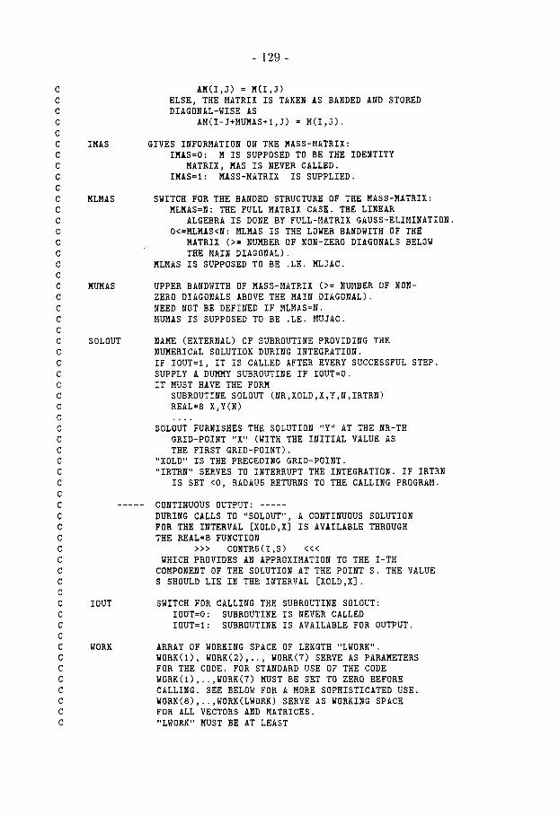
C CAN BOTH BE SCALARS OR ELSE BOTH VECTORS OF LENGTH N.CC ITOL SWITCH FOR RTOL AND ATOL:C ITOL=O: BOTH RTOL AND ATOL ARE SCALARS.C THE CODE KEEPS, ROUGHLY, THE LOCAL ERROR OFC Y(I) BELOW RTOL*ABS(Y(I))+ATOLC ITOL=1: BOTH RTOL AND ATOL ARE VECTORS.C THE CODE KEEPS THE LOCAL ERROR OF Y(I) BELOWC RTOL(I)*ABS(Y(I))+ATOL(I).CC JAC NAME (EXTERNAL) OF THE SUBROUTINE WHICH COMPUTESC THE PARTIAL DERIVATIVES OF F(X,Y) WITH RESPECT TO YC (THIS ROUTINE IS ONLY CALLED IF IJAC=1; SUPPLYC A DUMMY SUBROUTINE IN THE CASE IJAC=O).C FOR IJAC=1, THIS SUBROUTINE MUST HAVE THE FORMC SUBROUTINE JAC(N,X,Y,DFY,LDFY)C REAL*8 X,Y(N),DFY(LDFY,N)C DFY(1,1)= ...C LDFY, THE COLUMN-LENGTH OF THE ARRAY, ISC FURNISHED BY THE CALLING PROGRAM.C IF (MLJAC.EQ.N) THE JACOBIAN IS SUPPOSED TOC BE FULL AND THE PARTIAL DERIVATIVES AREC STORED IN DFY ASC DFY(I,J) = PARTIAL F(I) / PARTIAL Y(J)C ELSE, THE JACOBIAN IS TAKEN AS BANDED ANDC THE PARTIAL DERIVATIVES ARE STOREDC DIAGONAL-WISE ASC DFY(I-J+MUJAC+1,J) = PARTIAL F(I) / PARTIAL Y(J).CC IJAC SWITCH FOR THE COMPUTATION OF THE JACOBIAN:C IJAC=O: JACOBIAN IS COMPUTED INTERNALLY BY FINITEC DIFFERENCES, SUBROUTINE "JAC" IS NEVER CALLED.C IJAC=1: JACOBIAN IS SUPPLIED BY SUBROUTINE JAC.CC MLJAC SWITCH FOR THE BANDED STRUCTURE OF THE JACOBIAN:C MLJAC=N: JACOBIAN IS A FULL MATRIX. THE LINEARC ALGEBRA IS DONE BY FULL-MATRIX GAUSS-ELIMINATION.C O<=MLJAC<N: MLJAC IS THE LOWER BANDWITH OF JACOBIANC MATRIX (>= NUMBER OF NON-ZERO DIAGONALS BELOWC THE MAIN DIAGONAL).CC MUJAC UPPER BANDWITH OF JACOBIAN MATRIX (>= NUMBER OF NON-C ZERO DIAGONALS ABOVE THE MAIN DIAGONAL).C NEED NOT BE DEFINED IF MLJAC=N.CC MAS,IMAS,MLMAS, AND MUMAS HAVE ANALOG MEANINGSC FOR THE "MASS MATRIX" (THE MATRIX "M" OF SECTION IV.8):CC MAS NAME (EXTERNAL) OF SUBROUTINE COMPUTING THE MASS-C MATRIX M.C IF IMAS=O, THIS MATRIX IS ASSUMED TO BE THE IDENTITYC MATRIX AND NEED NOT BE DEFINED;C SUPPLY A DUMMY SUBROUTINE IN THIS CASE.C IF IMAS=1, THE SUBROUTINE MAS IS OF THE FORMC SUBROUTINE MAS(N,AM,LMAS)C REAL*8 AM(LMAS,N)C AM(1,1)= ....C IF (MLMAS.EQ.N) THE MASS-MATRIX IS STOREDC AS FULL MATRIX LIKE

CCCCCCCCCCCCCCCCCCCCCCCCCCCCCCCCCCCCCCCCCCCCCCCCCCCCCCCCCCC

IMAS

MLMAS

MUMAS

SoLoUT

lOUT

WORK

- 129 -

AM (I ,J) = M(I,J)ELSE, THE MATRIX IS TAKEN AS BANDED AND STOREDDIAGONAL-WISE AS

AM(I-J+MUMAS+l,J) = M(I,J).

GIVES INFORMATION ON THE MASS-MATRIX:IMAS=O: M IS SUPPOSED TO BE THE IDENTITY

MATRIX, MAS IS NEVER CALLED.IMAS=l: MASS-MATRIX IS SUPPLIED.

SWITCH FOR THE BANDED STRUCTURE OF THE MASS-MATRIX:MLMAS=N: THE FULL MATRIX CASE. THE LINEAR

ALGEBRA IS DONE BY FULL-MATRIX GAUSS-ELIMINATION.O<=MLMAS<N: MLMAS IS THE LOWER BANDWITH OF THE

MATRIX (>= NUMBER OF NON-ZERO DIAGONALS BELOWTHE MAIN DIAGONAL).

MLMAS IS SUPPOSED TO BE .LE. MLJAC.

UPPER BANDWITH OF MASS-MATRIX (>= NUMBER OF NON-ZERO DIAGONALS ABOVE THE MAIN DIAGONAL).NEED NOT BE DEFINED IF MLMAS=N.MUMAS IS SUPPOSED TO BE .LE. MUJAC.

NAME (EXTERNAL) OF SUBROUTINE PROVIDING THENUMERICAL SOLUTION DURING INTEGRATION.IF IOUT=l, IT IS CALLED AFTER EVERY SUCCESSFUL STEP.SUPPLY A DUMMY SUBROUTINE IF IOUT=O.IT MUST HAVE THE FORM

SUBROUTINE SoLoUT (NR,XoLD,X,Y,N,IRTRN)REA1*8 X,Y(N)

SOLOUT FURNISHES THE SOLUTION "Y" AT THE NR-THGRID-POINT "X" (WITH THE INITIAL VALUE ASTHE FIRST GRID-POINT).

"XoLD" IS THE PRECEDING GRID-POINT."IRTRN" SERVES TO INTERRUPT THE INTEGRATION. IF IRTRN

IS SET <0, RADAU5 RETURNS TO THE CALLING PROGRAM.

CONTINUOUS OUTPUT: -----DURING CALLS TO "SOLOUT", A CONTINUOUS SOLUTIONFOR THE INTERVAL [XOLD,X] IS AVAILABLE THROUGHTHE REAL*8 FUNCTION

»> CoNTR5(I,S) «<WHICH PROVIDES AN APPROXIMATION TO THE I-TH

COMPONENT OF THE SOLUTION AT THE POINT S. THE VALUES SHOULD LIE IN THE INTERVAL [XOLD,X].

SWITCH FOR CALLING THE SUBROUTINE SoLoUT:IOUT=O: SUBROUTINE IS NEVER CALLEDIoUT=l: SUBROUTINE IS AVAILABLE FOR OUTPUT.

ARRAY OF WORKING SPACE OF LENGTH "LWoRK".WoRK(l), WORK(2), .. , WORK(7) SERVE AS PARAMETERSFOR THE CODE. FOR STANDARD USE OF THE CODEWORK(1), .. ,WORK(7) MUST BE SET TO ZERO BEFORECALLING. SEE BELOW FOR A MORE SOPHISTICATED USE.WORK(8), .. ,WORK(LWoRK) SERVE AS WORKING SPACEFOR ALL VECTORS AND MATRICES."LWoRK" MUST BE AT LEAST

- 130 -

SOPHISTICATED SETTING OF PARAMETERS

IF IMAS=OIF IMAS=1 AND MLMAS=N (FULL)IF MLMAS<N (BANDED MASS-M.)

IF MLJAC=N (FULL JACOBIAN)IF MLJAC<N (BANDED JAC.)

IF MLJAC=N (FULL JACOBIAN)IF MLJAC<N (BANDED JAC.)

N*(LJAC+LMAS+3*LE+8)+1

DECLARED LENGTH OF ARRAY "IWORK",

DECLARED LENGTH OF ARRAY "WORK".

WHERELHC=NLJAC=MLJAC+MUJAC+1

ANDLMAS=OLMAS=NLMAS=MLMAS+MUMAS+1

ANDLE=NLE=2*MLJAC+MUJAC+1

DECLARED LENGTH OF COMMON BLOCK»> COMMON /CONT/ICONT(3),RCONT(LRCONT) «<

WHICH MUST BE DECLARED IN THE CALLING PROGRAM."LRCONT" MUST BE AT LEAST

4*N+4 .THIS IS USED FOR STORING THE COEFFICIENTS OF THECONTINUOUS SOLUTION AND MAKES THE CALLING LIST FOR THEFUNCTION "CONTRS" AS SIMPLE AS POSSIBLE.

INTEGER WORKING SPACE OF LENGTH "LIWORK".IWORK(1),IWORK(2), ... ,IWORK(1) SERVE AS PARAMETERSFOR THE CODE. FOR STANDARD USE, SET IWORK(1), .. ,IWORK(1) TO ZERO BEFORE CALLING.IWORK(8), ... ,IWORK(LIWORK) SERVE AS WORKING AREA."LIWORK" MUST BE AT LEAST 3*N+1.

IN THE USUAL CASE WHERE THE JACOBIAN IS FULL AND THEHASS-MATRIX IS THE IDENTITY (IMAS=O), THE MINIMUMSTORAGE REQUIREMENT IS

LWORK = 4*N*N+8*N+1.

THE MAXIMUM NUMBER OF NEWTON ITERATIONS FOR THESOLUTION OF THE IMPLICIT SYSTEM IN EACH STEP.

THE DEFAULT VALUE (FOR IWORK(3)=0) IS 1.

THIS IS THE MAXIMUM NUMBER OF ALLOWED STEPS.THE DEFAULT VALUE (FOR IWORK(2)=0) IS 100000.

IF IWORK(1).NE.0, THE CODE TRANSFORMS THE JACOBIANMATRIX TO HESSENBERG FORM. THIS IS PARTICULARLYADVANTAGEOUS FOR LARGE SYSTEMS WITH FULL JACOBIAN,IT DOES NOT WORK FOR BANDED JACOBIAN (MLJAC<N)OR FOR IMPLICIT SYSTEMS (IMAS=1). IT ISALSO NOT RECOMMENDED FOR SPARSE JACOBIANS.

SEVERAL PARAMETERS OF THE CODE ARE TUNED TO MAKE IT WORKWELL. THEY MAY BE DEFINED BY SETTING WORK(1), .. ,WORK(1)AS WELL AS IWORK(1), .. ,IWORK(1) DIFFERENT FROM ZERO.FOR ZERO INPUT, THE CODE CHOOSES DEFAULT VALUES;

LIWORK

LWORK

LRCONT

IWORK

IWORK(2)

IWORK(3)

IWORK(1)

CCCCCCCCCCCCCCCCCCCCCCCCCCCCCCCCCCCCC

C ----------------------------------------------------------------------CCCCCCCCCCCCCCCCCCC

CC

- 131 -

WORK(6) AND WORK(6): IF WORK(5) < HNEW/HOLD < WORK(6), THEN THESTEP SIZE IS NOT CHANGED. THIS SAVES, TOGETHER WITH ALARGE WORK(3), LU-DECOMPOSITIONS AND COMPUTING TIME FORLARGE SYSTEMS. FOR SMALL SYSTEMS ONE MAY HAVEWORK(6)=1.DO, WORK(6)=1.2DO, FOR LARGE FULL SYSTEMSWORK(6)=O.99DO, WORK(6)=2.DO MIGHT BE GOOD.DEFAULTS WORK(5)=1.DO, WORK(6)=1.2DO

FOR

NUMERICAL SOLUTION AT X

X-VALUE FOR WHICH THE SOLUTION HAS BEEN COMPUTED(AFTER SUCCESSFUL RETURN X=XEND).

MAXIMUM STEP SIZE, DEFAULT XEND-X.

DIMENSION OF THE INDEX 3 VARIABLES. DEFAULT IWORK(7)=0.

UROUND, THE ROUNDING UNIT, DEFAULT 1.D-16.

STOPPING CRITERION FOR NEWTON'S METHOD, USUALLY CHOSEN <1.SMALLER VALUES OF WORK(4) MAKE THE CODE SLOWER, BUT SAFER.DEFAULT 0.03DO.

DIMENSION OF THE INDEX 2 VARIABLES. DEFAULT IWORK(6)=0.

THE SAFETY FACTOR IN STEP SIZE PREDICTION,DEFAULT 0.9DO.

DIMENSION OF THE INDEX 1 VARIABLES (MUST BE > 0).ODE'S THIS EQUALS THE DIMENSION OF THE SYSTEM.DEFAULT IWORK(6)=N.

IF IWORK(4).EQ.0 THE EXTRAPOLATED COLLOCATION SOLUTIONIS TAKEN AS STARTING VALUE FOR NEWTON'S METHOD.IF IWORK(4).NE.O ZERO STARTING VALUES ARE USED.THE LATTER IS RECOMMENDED IF NEWTON'S METHOD HASDIFFICULTIES WITH CONVERGENCE (THIS IS THE CASE WHENNSTEP IS LARGER THAN NACCPT + NREJCT).DEFAULT IS IWORK(4)=0.

DECIDES WHETHER THE JACOBIAN SHOULD BE RECOMPUTED;INCREASE WORK(3) , TO 0.1 SAY, WHEN JACOBIAN EVALUATIONSARE COSTLY. FOR SMALL SYSTEMS WORK(3) SHOULD BE SMALLER(O.001DO, SAY). NEGATIVE WORK(3) FORCES THE CODE TOCOMPUTE THE JACOBIAN AFTER EVERY ACCEPTED STEP.DEFAULT O.001DO.

THE FOLLOWING 3 PARAMETERS ARE IMPORTANT FORDIFFERENTIAL-ALGEBRAIC SYSTEMS OF INDEX> 1.THE FUNCTION-SUBROUTINE SHOULD BE WRITTEN SUCH THATTHE INDEX 1,2,3 VARIABLES APPEAR IN THIS ORDER.IN ESTIMATING THE ERROR THE INDEX 2 VARIABLES AREMULTIPLIED BY H, THE INDEX 3 VARIABLES BY H**2.

OUTPUT PARAMETERS

X

Y(N)

WORK(7)

WORK(4)

WORK(3)

WORK(1)

WORK(2)

IWORK(7)

IWORK(6)

IWORK(4)

IWORK(5)

CCCCCCCCCCCCCCCCCCCCCCCCCCCCCCCCCCCCCCCCCCCCCCCCCCC

CCCCCCC

- 132

REPORTS ON SUCCESS UPON RETURN:IDID=1 COMPUTATION SUCCESSFUL,IDID=-1 COMPUTATION UNSUCCESSFUL.

PREDICTED STEP SIZE OF THE LAST ACCEPTED STEPH

IDID

CCCCCCCC----------------------------------------------------------------------.C *** *** *** *** *** *** *** *** *** *** *** *** ***C DECLARATIONSC *** *** *** *** *** *** *** *** *** *** *** *** ***

IMPLICIT REAL*8 (A-H,O-Z)DIMENSION Y(N),ATOL(1),RTOL(1),WORK(LWORK),IWORK(LIWORK)LOGICAL IMPLCT,JBAND,ARRET,STARTNEXTERNAL FCN,JAC,MAS,SOLOUTCOMMON/STAT/NFCN,NJAC,NSTEP,NACCPT,NREJCT,NDEC,NSOL

C COMMON STAT CAN BE INSPECTED FOR STATISTICAL PURPOSES:C NFCN NUMBER OF FUNCTION EVALUATIONS (THOSE FOR NUMERICALC EVALUATION OF THE JACOBIAN ARE NOT COUNT ED)C NJAC NUMBER OF JACOBIAN EVALUATIONS (EITHER ANALYTICALLYC OR NUMERICALLY)C NSTEP NUMBER OF COMPUTED STEPSC NACCPT NUMBER OF ACCEPTED STEPSC NREJCT NUMBER OF REJECTED STEPS (DUE TO ERROR TEST),C (STEP REJECTIONS IN THE FIRST STEP ARE NOT COUNTED)C NDEC NUMBER OF LU-DECOMPOSITIONS OF BOTH MATRICESC NSOL NUMBER OF FORWARD-BACKWARD SUBSTITUTIONS, OF BOTHC SYSTEMS; THE NSTEP FORWARD-BACKWARD SUBSTITUTIONS,C NEEDED FOR STEP SIZE SELECTION, ARE NOT COUNTED

Bibliography

R. Alexander (1977): Diagonally implicit Runge-Kutta methods for stiff ODE's.SIAM J. Numer. Anal., vol. 14, pp. 1006-1021.

R.K. Alexander and J.J. Coyle (1988): Runqe-Kuiia methods and differential-algebraic systems. Report, Iowa State University, Ames.

V.I. Arnold (1978), Mathematical Methods of Classical Mechanics. Springer Ver-lag.

M. Berzins and R.M. Furzeland (1985): A user's manual for SPRINT - a versa-tile software package for solving systems of algebraic, ordinary andpartial differential equations: part 1 - algebraic and ordinary dif-ferential equations. Thornton Research Centre, Shell Research Ltd.TNER.85.058.

M. Berzins, P.M. Dew and A.J. Preston (1988): Integration algorithms for thedynamic simulation of production processes. Report 88.20, School ofComputer Studies, University of Leeds.

K.E. Brenan (1983): Stability and convergence of difference approximations forhigher-index differential-algebraic systems with applications in tra-jectory control. Doctoral thesis, Dep. Math., Univ. of California, LosAngeles.

K.E. Brenan, S.L. Campbell and L.R. Petzold (1989): . In preparation.

K.E. Brenan and L.R. Engquist (1988): Backward differentiation approximationsof nonlinear differential/algebraic systems. To appear in Math. Com-put.

K.E. Brenan and L.R. Petzold (1986): The numerical solution of higher index dif-ferential/algebraic equations by implicit Runge-Kutta methods. Pre-print UCRL-95905, Lawrence Livermore National Laboratory.

K. Burrage and L.R. Petzold (1988): On order reduction for Runge-Kutta meth-ods applied to differential/algebraic systems and to stiff systems ofODE's. Preprint UCRL-98046, Lawrence Livermore National Labo-ratory.

J .C. Butcher (1976): On the implementation of implicit Runge-Kutta methods.BIT, vol. 16, pp. 237-240.

J.C. Butcher (1987): The Numerical Analysis of Ordinary Differential Equations.John Wiley & Sons.

G.D. Byrne and A.C. Hindmarsh (1987): Stiff ODE solvers: a review of currentand coming attractions. J. Comput. Physics, vol. 70, pp. 1-62.

S.L. Campbell (1980): Singular Systems of Differential Equations. Pitman, Lon-don.

S.L. Campbell (1982): Singular Systems of Differential Equations II. Pitman,

- 134 -

London.

K. Dekker and J.G. Verwer (1984): Stability of Runge-Kutta Methods for StiffNon-linear Differential Equations. North-Holland, Amsterdam - NewYork - Oxford.

G. Denk and P. Rentrop (1989): Mathematical models in electric circuit simulationand their numerical treatment. Numerical Treatment of DifferentialEquations, Halle/DDR 1989, Teubner-Texte zur Mathematik.

P. Deuflhard, E. Hairer and J. Zugck (1987): One-step and extrapolation methodsfor differential-algebraic systems. Numer. Math., vol. 51, pp. 501-516.

P. Deuflhard and U. Nowak (1987): Extrapolation integrators for quasilinear im-plicit ODEs. In P. Deuflhard and B. Engquist (eds.), Large-ScaleScientific Computing. Birkhauser, Boston.

J.R. Dormand and P.J. Prince (1980): A family of embedded Runge-Kuttaformu-lae. J .Comp. Appl. Math. vol.6, pp.19-26.

A. Feng, C.D. Holland and S.E. Gallun (1984): Development and comparison ofa generalized semi-implicit Runge-Kutta method with Gear's methodfor systems of coupled differential and algebraic equations. Compo &Chern. Eng., vol. 8, pp. 51-59.

C. Fuhrer (1988): Differential-algebraische Gleichungssysteme in mechanischenMehrkorpersystemen: Theorie, numerische Ansiiize und Anwendun-gen. Doctoral thesis, Technische Universitat Miinchen.

S.E. Gallun and C.D. Holland (1982): Gear's procedure for the simultaneous so-lution of differential and algebraic equations with application to un-steady state distillation problems. Compo & Chem. Eng., vol. 6, pp.231-244.

F. Gantmacher (1960): The Theory of Matrices II. Chelsea, New York.

F. Gantmacher (1970): Lectures in Analytical Mechanics. Mir, Moscow.

W.B. Gragg (1965): On extrapolation algorithms for ordinary initial value prob-lems. SIAM J. Numer, Anal., vol, 2, pp. 384-404.

C.W. Gear (1971): Simultaneous solution of differential-algebraic equations. IEEETrans. Circuit Theory, vol. 18, pp. 89-95.

C.W. Gear (1988): Differential-algebraic equation index transformations. SIAMJ. Sci. Stat. Comp., vol. 9, pp. 39-47.

C.W. Gear (1989): Differential-algebraic equations, indices, and integral algebraicequations. To appear in SIAM J. Numer. Anal.

C.W. Gear, H.H. Hsu and L. Petzold (1981): Differential-algebraic equations re-visited. Proc. Numerical Methods for Solving Stiff Initial Value Prob-lems, Oberwolfach, BRD.

- 135 -

C.W. Gear, G.K. Gupta and B. Leimkuhler (1985): Automatic integration ofEuler-Lagrange equations with constraints. J. Compo Appl. Math.,vol. 12&13, pp. 77-90.

C.W. Gear and L.R. Petzold (1984): ODE methods for the solution of differen-tial/algebraic systems. SIAM J. Numer. Anal., vol. 21, pp. 716-728.

E. Griepentrog and R. Marz (1986): Differential-algebraic Equations and TheirNumerical Treatment. Teubner, Leipzig.

E. Hairer, Ch. Lubich and M. Roche (1988): Error of Runge-Kutta methods forstiff problems studied via differential algebraic equations. BIT, vol.28, pp. 678-700.

E. Hairer, S.P. Nersett and G. Wanner (1987): Solving Ordinary DifferentialEquations I. Nonstiff Problems. Springer Series in ComputationalMathematics, vol. 8, Springer Verlag.

E. Hairer and G. Wanner (1988): Radau5 - an implicit Runge-Kutta code. Report,Dept. de mathematiques, Universite de Ceneve.

A.C. Hindmarsh (1980): LSODE and LSODI, two new initial value ordinary differ-ential equation solvers. ACM-SIGNUM Newsletter 15, pp. 10-11.

E.-H. Horneber (1976): Analyse nichtlinearer RLCU-Netzwerke mit Hilfe dergemischten Potentialfunktion mit einer systematischen Darstellungder Analyse nichtlinearer dynamischer Neizuierke. FB: Elektrotech-nik, Universitat Kaiserslautern, Dissertation.

W.H. Hundsdorfer (1987): Stability results for O-methods applied to a class ofstiff differential-algebraic equations. Report NM-R8708, CWI, Am-sterdam.

A. Kveerne (1987): Order conditions for Runge-Kutta methods applied to dif-ferential-algebraic systems of index 1. Math. of Comput. No. 4/87,University of Trondheim.

A. Kveerne (1988): Runge-Kutta methods applied to fully implicit differential/al-gebraic equations of index 1. Math. of Comput , No. 1/88, Universityof Trondheim. To appear in Math. Compo

A. Kveerne (1988b): Runge-Kutta methods for the numerical solution of differen-tial-algebraic equations of index 1. Doctoral thesis, University ofTrondheim.

J.L. Lagrange (1788): Mecanique analytique. Paris

B.J. Leimkuhler, L.R. Petzold and C.W. Gear (1988): On the consistent ini-tialization of differential algebraic equations. Submitted to SIAM J.Numer. Anal.

P. Lotstedt and L. Petzold (1986): Numerical solution of nonlinear differentialequations with algebraic constraints I: Convergence results for back-

- 136 -

ward differentiation formulas. Math. Comput., vol 46, pp. 491-516.

Ch. Lubich (1988): h2-extrapolation methods for differential-algebraic systems.Report, lnst. f. Math. u. Geom., Universitat Innsbruck.

Ch. Lubich (1989): Linearly implicit extrapolation methods for differential-alge-braic systems. Numer. Math., vol. 55 , pp. 197-211.

Ch. Lubich and M. Roche (1989), Rosenbrock methods for differential-algebraicsystems with solution-dependent singular matrix multiplying the deri-vative. Submitted for publication in Computing.

R.E. O'Malley, Jr. (1988): On nonlinear singularly perturbed initial value prob-lems. SIAM Rev., vol. 30, pp. 193-212.

R. Marz (1985): On initial value problems in differential-algebraic equations andtheir numerical treatment. Computing, vol. 35, pp. 13-37.

R. Marz (1987): Higher index differential-algebraic equations: Analysis and nu-merical treatment. Preprint Nr. 159, Humboldt-Universitat Berlin,to appear in Banach Center Publications.

R. Marz (1989): Index-2 differential-algebraic equations. Results in Mathematics,vol. 15, pp.149-171.

M.L. Michelsen (1976): Semi-implicit Runge-Kutta methods for stiff systems, pro-gram description and application examples. Inst. f. Kemiteknik, Dan-marks tekniske Hejskole, Lyngby.

S.P. Norsett and P. Thomsen (1986): Local error control in SDIRK-methods. BIT,vol. 26, pp. 100-113.

J.M. Ortega and W.C. Rheinboldt (1970): Iterative Solution of Nonlinear Equa-tions in Several Variables. Academic Press, New York - San Fran-cisco - London.

A. Ostermann (1989): A half-explicit method for differential-algebraic systems ofindex 3. Report, Dept. de mathematiques, Universite de Geneve. Toappear in IMA J. of Numer. Anal.

C.C. Pantelides (1988): The consistent initialization of differential-alge braic sys-tems. SIAM J. Sci. Stat. Comput., vol. 9, pp. 213-231.

L.R. Petzold (1982): A description of DASSL: A Differential/Algebraic SystemSolver. Proceedings of IMACS World Congress, Montreal, Canada.

L.R. Petzold (1986): Order results for implicit Runge-Kutta methods applied todifferential/algebraic systems. SIAM J. Numer. Anal., vol. 23, pp.837-852.

L. Petzold and P. Ldtstedt (1986): Numerical solution of nonlinear differentialequations with algebraic constraints II: Practical implications. SIAMJ. Sci. Stat. Comput., vol. 7, pp.720-733.

A.J. Preston, M. Berzins, P.M. Dew and L.E. Scales (1989): Towards efficient

- 137 -

D.A.E solvers for the solution of dynamic simulation problems. Toappear in the proceedings of the IMA Computational ODE-conference1989, London.

P. Rentrop, M. Roche and G. Steinebach (1989): The application of Rosenbrock­Wanner type methods with stepsize control in differential­algebraicequations. To appear in Numer. Math.

W.C. Rheinboldt (1984): Differential­algebraic systems as differential equationson manifolds. Math. Comp., vol. 43, pp. 473-482.

R.E. Roberson and R. Schwertassek (1988): Dynamics of Multibody Systems.Springer-Verlag, Berlin.

M. Roche (1988a): Rosenbrock methods for differential algebraic equations. Nu-mer. Math., vol. 52, pp. 45-63.

M. Roche (1988b): Runge­Kutta methods for differential algebraic equations. Toappear in SIAM J. Numer. Anal.

M. Roche (1988c): Runge­Kutta and Rosenbrock methods for differential­algebraicequations and stiff ODEs. Doctoral thesis, Universite de Geneve.

M. Roche (1989), The numerical solution. of differential algebraic systems byRosenbrock methods. In Num. Treat. ofDiff. Equ., Halle 1989, Teubner-Texte zur Math., DDR.

J. Wittenburg (1977): Dynamics of Systems of Rigid Bodies. Teubner, Stuttgart.

J. Wittenburg (1989): Dynamik von Mehrkorpersystemen. GAMM Mitteilungen,Heft 1, pp. 40-57.

Subject index

Amplifier 108A-stability 19Asymptotic expansionfor index 1, 27for index 2, 40for index 3, 82for half-explicit methods 50,90

BDF methods 54,91,123B(p) 15,34,64Bushy trees 64

Classical order 25Codes 123Consistent initial values 2,99Constrained mechanical system 5Convergence 17,25,36,40,78,92C(1]) 15,34,64

Differential index 13Discharge pressure control 116Dynamic simulation problem 116D(e) 15,64

E, E2-expansion 9,10,19Electrical circuit 5,108,112Elementary differentials 56Error

error estimation 99,122error propagation 36, Lemma 4.5,6.5local error 34,76,122

Explicit Runge-Kutta methods 14,20,23Extrapolation methods 16,50,90,123Euler method 16

Gauss methods 16,45Gragg's method 21,50

Half-explicit methods

Euler 50,90mid-point rule 50Runge-Kutta 20,48,68

Homotopy 31,72

Implicit differential equation 1Implicit Euler method 16

asymptotic expansion 40Implicit function theorem 2,23,99Index

differential index 13index of nilpotency 12index-m-tractability 13perturbation index 1subject index 138

Invariance under transformation 4,30

Jacobian matrix 92

Lady Windermere's Fan 36Lagrange equations 6Lobatto IlIA methods 16,46Lobatto IIIB methods 16Lobatto IIIC methods 16,48Local error 34,76

Matrix pencil 12

Newton iterations 92Nonlinear Gaussian elimination 4

Orderclassical order 25stage order 25order of a tree 57order conditions 62,68

Order of convergencefor index 1, 25for index 2, 36,40

- 139-

for index 3, 78for half-explicit methods 48

Ordinary differential equation 1,14

Pendulum 8,102,118Perturbations 1,33,75Perturbation index 1Perturbed asymptotic expansion 40,82Projection 35,77,100

Quadrature formulas 15

Radau IA methods 16,47Radau I1A me thods 16,47Radau5 106,124Ring modulator 112Rosenbrock methods 29,54,123Runge-Kutta methods 14Runge-Kutta solution

existence 31,72uniqueness 31,72

Scalingof error estimates 102,104of linear systems 97

Simplified Newton iterations 92Simplifying assumptions 15,64Singly diagonally implicit RK 16,48Singularly perturbed problem 9,10,19Stability function 19,25Stage order 25Stiff pendulum 10,119Stiff problem 10

Transformation of systems 3,4,5Trapezoidal rule 14,16Trees (rooted) 56Two phase plug flow problem 106Two transistor amplifier 108

Van der Pol equation 121