1€¦ · web viewecology and conservation biology contain numerous examples of populations...

- 1 -

TIEETeaching Issues and Experiments in Ecology - Volume 9, November 2013

EXPERIMENTS

Teaching Exponential and Logistic Growth in a Variety of Classroom and Laboratory Settings

Barry Aronhime1*, Bret D. Elderd1, Carol Wicks2, Margaret McMichael3, Elizabeth Eich4

1Department of Biological Sciences, Louisiana State University, Baton Rouge, LA 70803

2Department of Geology & Geophysics, Louisiana State University, Baton Rouge, LA 70803

3Baton Rouge Community College, Baton Rouge, LA 70806

4Biochemistry and Cell Biology Department, Rice University, Houston, TX 77251

*Corresponding Author: [email protected]

ABSTRACTEcology and conservation biology contain numerous examples of

populations growing without bounds or shrinking towards extinction. For these populations, the change in the number of individuals generally follows an exponential curve. On the other hand, limited resources may keep population numbers in check and help maintain the population at the environment's carrying capacity. These density-dependent constraints on population growth can be described by the logistic growth equation. The logistic growth equation provides a clear extension of the density-independent process described by exponential growth. In general, exponential growth and decline along with logistic growth can be conceptually challenging for students when presented in a traditional lecture setting. Establishing a solid understanding of exponential and logistic growth, core concepts in population and community ecology, provides a foundation on which students can build on in future studies. The module described here, employed in either a laboratory or classroom setting is designed to actively engage students in building their understanding of exponential and logistic processes. The module includes components that address a variety of learning styles (visual and tactile, for example). The module consists of pre-module assessments of students’ prior knowledge, three short “chalk talks” on exponential and logistic growth, the activities, and post-module assessments.

TIEE, Volume 9 © 2013 – Barry Aronhime, Bret D. Elderd, Carol Wicks, Margaret McMichael, Elizabeth Eich, and the Ecological Society of America. Teaching Issues and Experiments in Ecology (TIEE) is a project of the Committee on Diversity and Education of the Ecological Society of America (http://tiee.esa.org).

mailto:[email protected]

- 2 -


The time required for the activity will vary depending on replication and depth of coverage, but will require at least 80 minutes. We recommend carrying out these exercises in either one laboratory period or two lectures. The activity is designed for students to work in groups. Each group is given a set of containers representing samples from a hypothetical population. Each container, representing different sampling times, contains a different, predetermined number of units (individuals from the population, represented by pieces of candy or beads). To explore exponential growth, the students count the individuals at each time point and use arithmetic and semi-log graph paper to plot the data. From the data and graph(s), the students determine whether their population is growing, declining, or being maintained at a stable size. The students can then be called upon to predict future population sizes. Exploration of the logistic equation follows similar methodology except population numbers plateau over time. The module, as a whole, is quite flexible and can be easily adapted to a variety of institutions, subjects, or course levels, depending upon the need of the class. It can also be applied to other fields, such as geology (e.g., decay of radioactive isotopes).

KEYWORD DESCRIPTORS Ecological Topic Keywords: exponential growth, exponential decay,

population ecology, density-independent growth, logistic growth, density-dependent growth

Science Methodological Skills Keywords: data collection, graphing data, data interpretation, quantitative analysis, making predictions

Pedagogical Methods Keywords: background knowledge, cooperative learning, group activity, formative assessment, summative assessment, problem-based learning, active learning

CLASS TIMEThe amount of in-class time depends upon the instructor's needs and goals. The core activity, during which students collect and graph the exponential data on arithmetic graph paper, can be completed within 50 minutes. Class or lab periods of 80 minutes provide sufficient time for students to create a second graph, on semi-log paper. The module can be expanded further, for a three hour ecology laboratory, for example, by including a section on regression where students estimate population growth rates directly from the data. The logistic growth portion will likely require an additional 20-30 minutes of class time.


http://tiee.esa.org/teach/teach_glossary.html#problem

http://tiee.esa.org/teach/teach_glossary.html#formative

http://tiee.esa.org/teach/teach_glossary.html#cooperative

http://tiee.esa.org/teach/teach_glossary.html#cooperative

http://tiee.esa.org/teach/teach_glossary.html#background_knowledge_probe

- 3 -


OUTSIDE OF CLASS TIMEEach student will need 30-60 minutes for reading assigned materials (chapters in text, laboratory manual) before class. For a full laboratory, the students can complete a homework assignment based on the data collected that day.

STUDENT PRODUCTSStudent groups construct a data table and graphs (regular arithmetic scale and semi-log scale) of the data, which can be submitted after class or used as a basis for an at home writing assignment. Students should also answer questions given by the instructor on notecards or via an automated response system.

SETTINGThis exercise can be used in any lecture classroom, large or small, or in a laboratory. All required items can be picked up at a local grocery or craft store.

COURSE CONTEXTThis module is malleable to both subject and class size. For example, it has been incorporated into senior level ecology lectures (25-50 students), senior ecology laboratories (12 students), freshmen non-majors biology lectures (>200 students), and biology labs at the community college level (24 – 30 students). This module was also modified to improve student understanding of the exponential decay of radioactive elements as applied to age dating in a geology lecture for non-geology majors. Students should work in groups of 3-4, regardless of class size. The module can and should be tailored to the course. Introductory students can get valuable information on graphing and making predictions from collecting and graphing the data. In senior level ecology lectures and laboratories, students can also plot the data on semi-log paper, use the y intercept as an estimate for the original population size, and use the slope of the line to estimate the instantaneous growth rate (r). Calculating the slope and intercept can either be done on the graph paper or using standard statistical packages (MS Excel or R [R Core Team, 2013] depending on class needs and the background of the students).

INSTITUTIONThe exercise has been applied successfully at institutions serving very different


- 4 -


student populations: Louisiana State University (LSU); Rice University (Rice); and, Baton Rouge Community College (BRCC). Both LSU and Rice are 4-year research institutions, but LSU is public and Rice is private. BRCC is a 2-year institution in an urban setting (Carnegie Foundation for the Advancement of Teaching).

TRANSFERABILITYThis module can be used at any institution of higher learning. All the materials required are inexpensive and can be found at a local grocery or craft store. Additionally, this exercise can be adapted for different levels of students. For students with weaker math backgrounds, the graphs allow them to define r visually. Students with stronger math backgrounds can further examine exponential and logistic growth by using the equations. Finally, topics can be extended, depending on the depth of the course, to introduce additional concepts such as the effects of environmental stochasticity on populations growing in a density-independent (i.e., exponential) or density-dependent (i.e., logistic) manner.

ACKNOWLEDGEMENTSWe would like to thank the Howard Hughes Medical Institute, and the National Academies Summer Institutes (Gulf Coast) for providing us with an environment to develop this activity. In particular, we would like to the thank Chris Gregg, Joe Siebenaller, and Bill Wischusen for their help and guidance throughout the development of this exercise. Louisiana State University College of Science, Baton Rouge Community College, and Rice University Weiss School of Natural Sciences provided us with the opportunity to attend the Summer Institutes and to test the module in our classrooms. We would also like to thank Molly Keller for helping to sort the candy.

SYNOPSIS OF THE EXPERIMENT

Principal ecological questions addressed for all studentsWhat is exponential growth? What is exponential decay? How do populations grow or decline exponentially? How can ecologists determine a population's health and project future population sizes? What is density-independent growth? What populations are best described by this model of growth? What is density-dependent growth? What is logistic growth? What differences in habitat allow for exponential vs. logistic growth?


- 5 -


Principal ecological questions addressed for all senior ecology studentsHow are logarithms useful in biology? How can ecologists estimate future population sizes mathematically?

What HappensAll classes

First, the students are asked a few pre-activity questions to assess their prior knowledge. Their responses can be recorded electronically, using a student response system (e.g., clickers) or on note cards. Afterwards, a short “chalk talk” introduces the students to population growth in general and to exponential growth more specifically. Each group of students is given arithmetic graph paper (and semi-log for senior ecology students), a notecard, and five population samples: sandwich bags with previously counted amounts of candy (we used “Skittles ®”) or beads. Each piece of candy or bead represents, for example, one bacterium. Each sandwich bag is labeled with sampling time (e.g., 0600, 0800, 1000, 1200, and 1400 hours). We used a deterministic model, with a known initial population size and growth rate, to estimate the number of bacteria at each interval. This can be modified to include stochastic variation in population numbers due to environmental noise, thus introducing students to the identification of patterns when noise is present.

Students first examine the bags and record if they think that the size of the bacterial population is increasing, decreasing, or remaining constant. Students then open the bags, count the individuals, and record the data in a table. Students use the data table to draw a curve on the arithmetic graph paper and determine if the population is increasing, decreasing or stable. If the population is increasing or decreasing, students describe the rate at which the population is increasing or decreasing (e.g., linear, exponential). Students are then given a sixth bag with the next time interval (e.g., 1600 hours) and asked to use their graph to predict the number of individuals that would be obtained in the sixth sample (i.e., the number of candies that should go into that bag). The students can turn in their notecard with all of the information they have recorded, including how many bacteria should be in the sixth bag. If the answer is correct, the students count out the appropriate amount of candy and take them home.

Additional procedure for senior ecology lecture and laboratory students

For senior level ecology students, it is appropriate to point out the difficulty in projecting from an exponential curve. The students can then plot their data on semi-log paper and estimate population size at time six based on the new graph. Plotting the data on semi-log paper will result in a straight line from which the


- 6 -


students can make a more accurate estimate. They can also be asked to find the instantaneous growth rate (slope of the line) and the initial population size (y-intercept). Students can then be asked to insert their estimates of the intercept and slope in the exponential growth equation logNt = logN0 + rt to estimate future population size. Ecology laboratory students may use the data in any software package (e.g., Excel or R) that calculates regression statistics to obtain estimates of the slope and the intercept. This will work especially well when assuming that population numbers vary due to stochasticity. Introductory biology students, in our experience, were not comfortable with logarithms and thus we did not extend the exercise beyond graphing on arithmetic paper.

Additional procedure for ecology laboratory and a second lecture for the other courses

A natural follow up to a discussion of exponential growth is a discussion of logistic growth. We feel that covering both topics is possible in a three hour laboratory setting, but not in a 50-80 minute lecture. The logistic growth exercise should be carried out in a second lecture. The procedure mimics the basic exponential growth procedure in that students will graph population size from five time intervals, but students are also given time intervals 6, 7, and 8. The number of Skittles in these time intervals should be similar, indicating that growth has leveled off. Again, stochasticity can be included in the population numbers to illustrate the effects of environmental variation on populations at carrying capacity.

Experiment ObjectivesUpon completion of this exercise, all students should be able to:

1) Plot data on a graph2) Make predictions of future population size based on data acquired3) Be able to identify patterns even when there is biological variation4) Identify when populations are growing at an exponential rate5) Identify when populations are growing at a logistic rate6) Differentiate between the exponential and logistic growth models in curve

shape, equations, predicted future population sizes, and habitat characteristics (i.e., resource availability)

7) Define (verbally and graphically) a carrying capacity

Senior level ecology students should also be able to:8) Calculate and interpret the instantaneous growth rate9) Know a practical application for logarithms10) Use MS Excel or R to estimate N0 and r


- 7 -


11) Calculate r and Nt mathematically

Equipment/ Logistics RequiredAll coursesIndex cardsSandwich bagsCandy or beadsMarkersLinear graph paperPencil

Additional materials for senior ecology lecture and laboratory* studentsSemi-log graph paperComputers with MS Excel or R

Summary of What is DueAll courses

In our trials, the students turned in the answers to the pre and post exercise questions, graphs, and notecards with their statements of the direction of population growth and estimates of the population size at the sixth time interval for an exponentially growing population. Students should also turn in graphs and notecards with answers to questions for the logistic growth portion as well.

Additional work for senior ecology laboratory students Especially in the ecology lab where each group would have six

populations, this project could be expanded into written assignments such as a homework assignment. In this lab situation, we recommend that each group of students have different candy populations. Then the data can be pooled across groups with each group treated as a replicate. Students can use those data to make graphs and predict future population sizes using MS Excel or R. We have included a possible homework assignment for the laboratory students with possible point values.

DETAILED DESCRIPTION OF THE EXPERIMENT

IntroductionIn 1798 Thomas Malthus’ classic An Essay on the Principle of Populations

introduced the world to the concept of exponential population growth. The idea


- 8 -


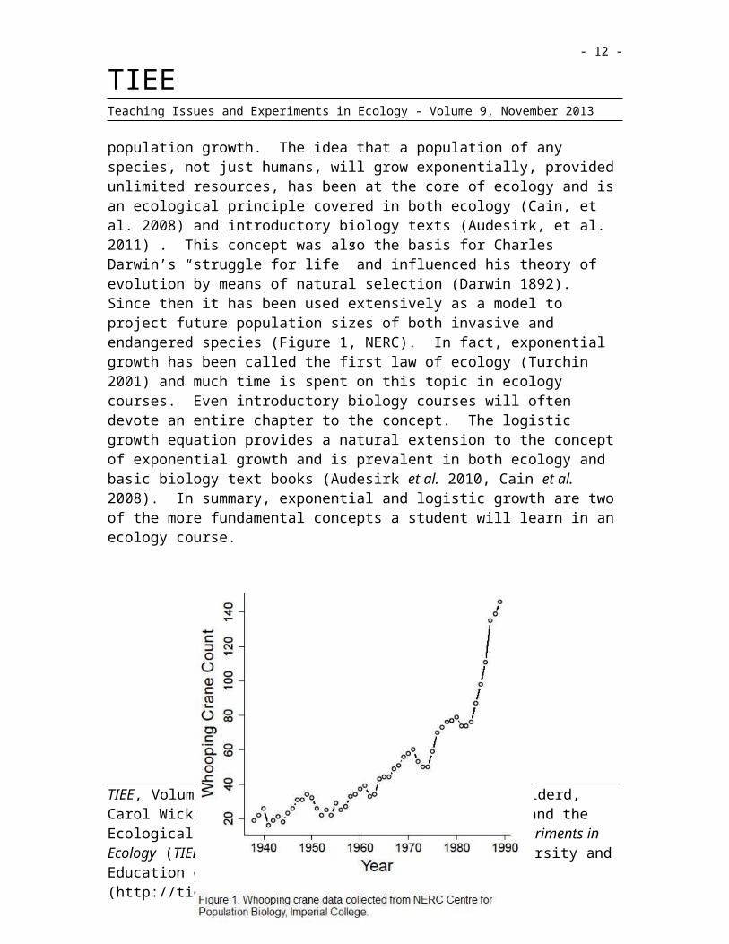
that a population of any species, not just humans, will grow exponentially, provided unlimited resources, has been at the core of ecology and is an ecological principle covered in both ecology (Cain, et al. 2008) and introductory biology texts (Audesirk, et al. 2011) . This concept was also the basis for Charles Darwin’s “struggle for life” and influenced his theory of evolution by means of natural selection (Darwin 1892). Since then it has been used extensively as a model to project future population sizes of both invasive and endangered species (Figure 1, NERC). In fact, exponential growth has been called the first law of ecology (Turchin 2001) and much time is spent on this topic in ecology courses. Even introductory biology courses will often devote an entire chapter to the concept. The logistic growth equation provides a natural extension to the concept of exponential growth and is prevalent in both ecology and basic biology text books (Audesirk et al. 2010, Cain et al. 2008). In summary, exponential and logistic growth are two of the more fundamental concepts a student will learn in an ecology course.

While understanding exponential and logistic growth is vital to the students’ understanding of ecology, in our experience, these concepts can be


- 9 -


challenging for many students. The challenging nature of the concepts originates from the students’ mathematics background and the abstract nature of the concepts. Few students in our classes were introduced to exponents and logarithms in high school. Due to the lack of familiarity with exponents, many students struggle with nonlinear relationships (e.g., Figure 1). To move exponential growth out the abstract and into the concrete and tangible, this module was developed during one of the National Academies Summer Institutes on Undergraduate Education sponsored by the Howard Hughes Medical Institute.

The module is designed to help students with a diverse set of learning styles. It employs tactile and visual senses – students handle the individual units (candy or beads) and manually graph the data – as they gain a solid foundation for future biological and ecological studies and a better understanding of the material. Please read “Chalk Talk One” and “Chalk Talk Three” for further details on deriving the exponential and logistic growth equations.

Materials and Methods

Advised Methods for All Courses 1) Please answer the following questions on a notecard and submit your

answers to the instructor: a. A (population, community, ecosystem, biome) is defined as a group

of individuals of a single species that occupies the same general area.

b. A population will grow when (b>d, b<d, b=d).c. A population in an environment with unlimited resources will grow

(exponentially, logistically).d. If a population grows at a rate of N = 2t, where t is the sampling

time interval, what is N at sampling time 10?2) Listen to the instructor’s lecture “Chalk Talk One”. 3) Gather in a group of four and send one representative to get five

sandwich bags with differing amounts of candy from the instructor. The bags are labeled with a military time. The time represents when the bacterial colony was sampled. Each candy represents one bacterium.

4) Examine the samples. First look at your bags to see if the populations are increasing, decreasing or staying stable.

5) Count the individuals at each sampling time and fill in the data table provided by your instructor:


- 10 -


6) Graph the data. Which data belong on what axis? How do you know?

7) Using the graph you created in step 6, predict the population size at the sixth time point.

8) A representative from each group should draw their graph on the board (or ELMO/overhead projector) and state if their population was increasing, decreasing, or staying stable.

9) Enter into a class discussion of you results. Why, biologically, are some curves not as smooth as others?

10) Answer the following wrap up questions on a notecard:a) If r is positive, the population will (grow, stay the same, or decline).b) If r is positive, the population’s birth rates will be (less than, equal to, or greater than) the death rates.c) Which of the following curves most closely resembles human population growth (linear, logistic, exponential, extra-exponential)? This question is particularly effective if they have at least seen population growth plotted on semi-log paper.

Additional Advised Methods for Senior Ecology Lecture and LaboratoryStudents should perform steps 1-8 as in the other course11) Answer the following question on a notecard:

a. log10(100)= (0.01,0.1, 2, 10).12) Enter a class discussion with the instructor. How confident do you

feel about your estimate of future population size? Did you find it difficult to estimate the next time interval with the exponential curve? Did you make any assumptions about the shape of the curve?

13) Listen to the instructor’s lecture “Chalk Talk Two” and listen to the explanation of graphing on semi-log paper.

14) Graph the same data as before on semi-log paper.15) Predict population size at time six using the semi-log paper. Which

do you think provided for a more accurate prediction, linear graph paper or semi-log paper?

16) Think about the line you drew. What is the biological meaning of slope of that line? What is the biological meaning of the y-intercept?

Advised methods for Logistic Growth (all courses)17) Are populations capable of indefinite exponential growth? Write your

answer on a notecard.18) Logistic growth – pay attention to the instructor’s “Chalk Talk Three”

and be prepared to answer questions.


- 11 -


19) Gather in a group of four and send one representative to get eight sandwich bags with differing amounts of candy from the instructor. The bags are labeled with a military time. The time represents when the bacterial colony was sampled. Each candy represents one bacterium.

20) Examine the samples. First look at your bags to see if the populations are increasing, decreasing or staying stable.

21) Count the individuals at each sampling time and fill in the data table provided by your instructor:

22) Graph the data. Which data belong on what axis? How do you know?

23) Using the graph you created in step 21, predict the population size at the ninth time point.

24) A representative from each group should draw their graph on the board (or ELMO/overhead projector) and state if their population was growing at an exponential or logistic rate. Now estimate K based on your graph.

25) Which model (exponential or logistic) do you think is more commonly found in nature?

26)What is density-independent vs. density-dependent growth?27)After introduction of density-dependent growth (via the logistic growth

equation), how does population growth rate change as the population size increases for both density-independent and density-dependent growth?

28) What habitat differences would lead to logistic growth rather than exponential growth?

Homework for Senior Ecology Laboratories - Use MS Excel or R and the Equations in the “Chalk Talks.”

a. Using the raw data you collected today, make graphs (label your axes and include figure captions) in MS Excel or R. You should have seven graphs (1 for each of your group’s six exponential growth curves and one for your group’s logistic growth curve). Copy those graphs and paste them into a MS Word document. (5 pts. per figure)

b. Using what you learned in “Chalk Talk Two” and regression statistics in MS Excel or R, report r and N0 for each of the 7 populations. (5 pts. per population)

c. A bacterial colony starts with 100 individuals and its population size at sampling time 1000 (hrs.) was 200,000. What is r for this


- 12 -


population? What would the bacterial colony’s population size be after 1 day (sampling time 2400)? (5 pts.)

d. Calculate the population size at year seven of a lion population with an initial population size of 20 and an instantaneous growth rate of 0.1 (rounded to the nearest whole number). (5 pts.)

e. The endangered purple falcon, which is endemic to your state, had a population size of 100 individuals in 2012. The population's instantaneous growth rate over the past decade has been 0.05 assuming a continuously growing population. Delisting of the falcon from the Endangered Species List can occur when the population reaches 1000 individuals. Using the density-independent population growth equation, when should the falcon be delisted? (10 pts.)

f. A population of common red-bellied snipe is limited by the number of nesting sites in their habitat. Thus, they grow according to the density-dependent logistic growth equation. Calculate the population growth rate for snipe populations of 25 and 75 given their instantaneous growth equals 0.1 and their carrying capacity equals 100. Are the growth rates the same or different? Why? (10 pts.)

Questions for Further Thought and Discussion: Questions for all students1) How useful of a tool is this for ecology or conservation biology? Is it just an

abstract concept or does it have any real-world applicability?2) When examining real-world data (e.g., Figure 1), why don't populations fit the

line exactly? What processes might allow populations to have more or less individuals than expected when sampled?

3) Why aren’t populations capable of indefinite exponential growth?

Additional question for senior ecology students 4) How are logarithms used in other fields of science?5) Based on what you’ve learned about population growth and resources, do

you think human populations can grow exponentially indefinitely? Explain your answer.

References and Links: Audesirk, T, G Audesirk, BE Byers. 2010. Biology: life on earth with physiology.

Pearson. San Francisco.


- 13 -


Cain, ML, WD Bowman, SD Hacker. 2008. Ecology. Sinauer Associates, Inc. Sunderland, MA.

Carnegie http://classifications.carnegiefoundation.org. Accessed 9/3/2013.Darwin, CR. 1892. Selected letters on evolution and origin of species with an

autobiographical chapter. Ed. F Darwin. Page 42.Malthus,T. 1798. An essay on the principle of population. London.Turchin, P. 2001. Does population ecology have general laws? Oikos 94:17-26.NERC Centre for Population Biology, Imperial College (2010). The Global

Population Dynamics Database Version 2.R Core Team. 2013. R: A Language and Environment for Statistical Computing.

Vienna, Austria: R Foundation for Statistical Computing. www.R-project.org. (accessed 9/3/13)

For more sample problems on exponential growth, please visit the following websites:http://www.worldbank.org/depweb/english/modules/social/pgr/texta.html (accessed 9/3/13)http://serc.carleton.edu/quantskills/methods/quantlit/popgrowth.html (accessed 9/3/13)www.waynesword.palomar.edu/lmexer9.htm (accessed 9/3/13)

Tools for Assessment of Student Learning Outcomes: Depending upon the needs of the class, the assessment tools can vary. At

the most basic level, the graphs drawn as a part of the exercise can be used to assess student learning. If the instructor wishes for a more detailed assessment, the graphs along with additional questions for further thought can be assigned as part of a take-home write-up or a lab report. Students should also be asked to interpret growth curves and predict future population sizes on exams. Lastly, when population estimates include environmental variation, the students can compare the estimates of r taken from 1) visually inspecting the graph and 2) using the exponential growth equation using the slope of the graph to see how different (or similar) the estimates might be.


http://www.waynesword.palomar.edu/lmexer9.htm

http://serc.carleton.edu/quantskills/methods/quantlit/popgrowth.html

http://www.worldbank.org/depweb/english/modules/social/pgr/texta.html

http://www.R-project.org/

http://classifications.carnegiefoundation.org/

- 14 -


NOTES TO FACULTY

Comments on Challenges to Anticipate and Solve:

In our freshmen courses, many of the students were unfamiliar with logarithms. This was an unexpected challenge and was part of the reason for removing that section from the non-majors course. However, given sufficient time the concept of logarithms can be easily taught to non-majors but might require an extra class period for the exercise. For upper-level major courses a refresher on logarithms and semi-log plots may be required. This was the biggest obstacle we found in implementing this exercise.

Comments on Introducing the Experiment to Your Students:

1) We advise beginning the exercise with clicker questions to assess the prior knowledge of the students where they record answers using clickers or notecards. Questions should address population growth, decline, and stability as well as basic logarithms (senior ecology students only). After prior knowledge has been assessed, a short chalk talk on factors that determine population growth should be given (see Chalk Talk One) before starting the exercise. Prior knowledge assessment can also be a great way to jump-start a discussion on population dynamics. Some of the clicker questions asked are given below. Note the correct answers are in bold.

a) A (population, community, ecosystem, biome) is defined as a group of individuals of a single species that occupies the same general area.b) A population will grow when (b>d, b<d, b=d).c) A population in an environment with unlimited resources will grow (exponentially, logistically).d) If a population grows at a rate of N = 2t, where t is the sampling time interval, what is N at sampling time 10? 1024.

2) Give each group five sandwich bags with differing amounts of candy. The bags are labeled with sampling time (0600, 0800, 1000, 1200, 1400). Again, for a three hour laboratory exercise, each group should get six populations with five bags in each population.

3) Vary the population growth among the groups. In our study, there were six treatments: exponential growth, exponential growth with variation, exponential decay, decay with variation, stable population, and stable population with variation.

4) Examine the samples. The students first look at their bags to see if the populations are increasing, decreasing or are stable. By using their visual


- 15 -


sense, the change in the number of individuals over time becomes more concrete.

5) Count the individuals at each sampling time and create a data table. The students then count the candy in the bags. Note that counting them within the bags can be more difficult with the high-density populations.

6) Graph the data. Students then graph the data (Figure 2). Senior ecology students should not be given any guidance as to what data belong on what axis. In the non-majors course, the question of what data belong on which axis should be addressed first.

7) Predict the population at the sixth time point. After students finish graphing the data, they predict the number of candies at time six.

8) Present results to other groups. Representative groups draw their graphs on the board (or ELMO/overhead projector) and state if their population size was increasing, decreasing, or stable. We also used this time to discuss biological variation.

Advised Methods for Senior Ecology Class Students should perform steps 1-8 as in the other courses.

9) A class discussion ensues about the difficulty of estimating future population sizes from an exponential curve. Logarithms and their use are discussed following a short chalk talk on the relationship between logarithms and population growth (See Chalk Talk Two). Students are given semi-logarithmic paper on which to plot their data. Semi-log paper needs to be explained to the students. They are likely unfamiliar with it.

10) Students graph the data on semi-log paper.11) Students predict population size at time six using the semi-log paper and

state whether arithmetic or semi-log paper provides a more accurate prediction.

12) The growth equation is placed on the board and comparisons made between the growth equations and the equation of a line. The class discusses the line drawn on the semi-log paper. From a biological perspective, what does the slope of the line represent? What does the y-intercept represent? Segue to “Chalk Talk Three” by asking students about exponential growth. Are populations capable of indefinite exponential growth? They should record their answer and then listen to “Chalk Talk Three.”

13) Chalk Talk Three is given.14) Students gather in groups of four and send one representative to get

eight sandwich bags with differing amounts of candy from the instructor. The bags labeled with a military time. The time represents when the bacterial colony was sampled. Each candy represents one bacterium.


- 16 -


15)Students first examine the samples and record if the populations are increasing, decreasing or staying stable.

16)Students count the individuals at each sampling time and fill in the data table provided by the instructor:

17)Students graph the data. By this point all students should know which data belong on what axis and not be given guidance.

18) Students use their graph to predict the population size at the ninth time point.

19) A representative from each group draws their graph on the board (or ELMO/overhead projector) and states if their population was growing at an exponential or logistic rate (will be logistic). You may consider giving some groups exponentially growing populations for comparison.

20) Students then answer the following questions and class discussion follows.

a. Which model (exponential or logistic) do you think is more commonly found in nature?

b. What is density-independent vs. density-dependent growth?c. How does population growth rate change as the population size

increases for both density-independent and density-dependent growth?

d. What habitat differences would lead to logistic growth rather than exponential growth?

.

Comments on the Data Collection and Analysis Methods:

Depending on the size of your class, you may need several hours to get the sandwich bags of candy or beads together and organized. Data collection by the students is relatively easy.

Comments on Questions for Further Thought:

Question 1 ties the mathematics back to the biology to show the students the two are interconnected. Without the language of math, we can be at a loss for describing patterns in nature. It can be an opportune time to talk more about the types of natural conditions under which these patterns are most likely to be observed (e.g., when a population newly invades an area, when a population is being driven to extinction, and the onset of a bacterial infection in a human being).

Question 2 allows for a discussion on variation or stochasticity in population numbers. In upper-level classes, the instructor can bring up the three main types of stochasticity that affect population numbers (environmental,


- 17 -


demographic, and genetic) and when they might be important. For more advanced students, the instructor can also touch on measurement error.

Question 3 addresses issues related to density-dependent population growth, which is often the next topic covered in ecology classes. Question 3 allows the students to think about limits to population growth such as food or space.

Question 4 provides the opportunity to talk about other topics outside of population growth such as the importance of radioactive decay as fundamental to age dating geological materials.

Comments on the Assessment of Student Learning Outcomes:

Graphing and clicker question responses provide data for formative assessment of student learning. Homework further emphasizes the interpretation of the growth curves and the implications for future population size. Exam questions may be used to obtain summative assessment of student learning: for example, students may be asked to create or interpret growth curves and predict future population size(s). The data or curves presented to the students could include biological variation to ensure that they can interpret a signal in the presence of environmental noise. Students should also be asked to compare and contrast the density-independent and density-dependent growth curves. These summative assessment questions will indicate long-term retention of the concept.

Comments on Formative Evaluation of this Experiment:

Clickers or notecards are easy-to-use tools that permit real-time assessment of students’ understanding of exponential growth. For example, students can be asked to relate equations to curves using either tool. These formative assessment tools allow us to gauge whether the students have achieved the goals of the exercise, what topics should be covered in further detail, and also stimulate further discussion on the topic.At the end of the exercise, we asked a series of clicker questions. Note the correct answers are in bold.

Questions for all studentsa) If r is positive, the population will (grow, stay the same, or decline).b) If r is positive, the population’s birth rates will be (less than, equal to, or greater than) the death rates.c) Which of the following curves most closely resembles human population growth (linear, logistic, exponential, extra-exponential)? This question is


- 18 -


particularly effective if they have at least seen population growth plotted on semi-log paper.

Questions for senior level ecology laboratory studentsd) If a bacterial colony starts with 100 individuals and its population size at sampling time 1000 (hrs) was 20,000; what is r? 0.53. What would the bacterial colonies population size be after 1 day (sampling time 2400)? 33,436,598.e) Calculate the population size at year seven of a lion population with an initial population size of 20 and an instantaneous growth rate of 0.1 (rounded to the nearest whole number). N7 = 40.f)The endangered purple falcon, which is endemic to your state, had a population size of 100 individuals in 2012. The population's instantaneous growth rate over the past decade has been 0.05 assuming a continuously growing population. Delisting of the falcon from the Endangered Species List can occur when the population reaches 1000 individuals. Using the density-independent population growth equation, when should the falcon be delisted? 2058.g) A population of common red-bellied snipe is limited by the number of nesting sites in their habitat. Thus, they grow according to the density-dependent logistic growth equation. Calculate the population growth rate for snipe populations of 25 and 75 given that their instantaneous growth equals 0.1 and their carrying capacity equals 100. Are the growth rates the same or different? Why? Population growth rate is the same, 1.875.

Comments on Translating the Activity to Other Institutional Scales or Locations:

This exercise has already been used at public and private 4-year research institutions as well as a 2-year institution. It has been used in classes as small as 14 and as large as 220. The exercise has also been used in geology classes to explain radioactive decay. This is a very malleable exercise that can be used in most classroom settings. The exercise should be adjusted based on the size and the duration of the class. For example, in a large (>100 students) lecture (50 – 70 minutes) each group was given one population to count and graph. Limiting the groups to one population decreases prep time for the instructor and allows enough time in class for the exercise to be completed. In our large lecture, 50 populations needed to be created which required several hours and some assistants for preparation. In small labs (~ 14 students; 170 minutes) each group was given six populations to count and graph. In labs, a greater emphasis can


- 19 -


be placed on replication and the differences among the six different populations. In our lab, 18 populations needed to be created to complete the exercise.


- 20 -


STUDENT COLLECTED DATA FROM THIS EXPERIMENT

.

Description of other Resource Files

Chalk Talk OneIn biology, population size changes over time. By simply counting the number of individuals in a population over time, we can learn a great deal. If samples of a population are taken over a long time, we can determine whether it is growing, shrinking, or staying stable. The data can then be used to calculate a


- 21 -


population's growth rate and predict population size in the near future. First, we have to be able to interpret our count data. We can simply write out how populations change in size using words. For example,

Change in Population Size = Births - Deaths + Immigrants - Emigrants. (1)

Here we assume that population growth is dictated by four processes where two of these processes, birth and immigration, increase population numbers and two of these processes, death and emigration, lead to a decrease in numbers. This assumes that the population is open to individuals coming and going. If the population is closed, then population growth is simply the difference between the number of births and deaths. If births are greater than deaths, then the population grows; whereas, if births are less than deaths, then the population declines. Lastly, if births equal deaths, then the population stays the same size and is considered stable over time. Rather than describing in words what happens, we can write a simple equation:

(2)

Here N is the change in population size, B is the number of births in the population, and D is the number of deaths. Instead of talking about the number of births or deaths in the population as a whole, we can also talk about the per capita birth rate (b) and per capita death rate (d). If reproduction and death are continuous (i.e., individuals are born and die throughout the time sampled), we can describe population growth rate using a simple exponential equation where:

(3)

where dN/dt is the instantaneous change in population numbers over the change in time, t. The term b - d is the instantaneous change in the population per individual per unit time, which we can abbreviate with r. If r, the instantaneous growth rate, is greater than zero, the population grows since r times N is positive. If r is less than zero, the population declines. An r equal to zero results in a stable population (Note: concrete examples can be given on the board. Also, if students are unfamiliar or uncomfortable with calculus, G can be substituted for dN/dt.) If we then integrate equation 3 using calculus, we arrive at:

Nt = N0ert (4)


- 22 -


which describes population size at any time interval. Where Nt is population size at time t, N0 is the initial population size, and e is the base of the natural logarithm. Equation 4 results in populations that either grow, shrink, or stay the same over time depending on the value of r (Figure Chalk1).

Chalk Talk Two for Ecology Students Now, as we have seen, it can be hard to predict the number of individuals

at the next time interval when a population is growing exponentially on arithmetic graph paper; however, life becomes easier if we use logarithms or semi-log graph paper. Let's first review logarithms. What would be the logarithm of 100? If we use the common logarithm, we are using a logarithm to the base 10. Therefore:

log10(100) = log10(102)=2.

For our exponential growth equation, we need to use a base of e to go from an exponential curve to a straight line, where the logarithm of the growth equation becomes:

loge(Nt) = loge(N0ert). (5)

Instead of base of 10, we have a base of e, which is called the natural logarithm. The next step is to simplify the equation given our knowledge of logarithms. First, we know that log(ab) = log(a) + log(b). Second, we know the loge(e) = 1 just like the log10(10) = 1. Given this, equation 5 simplifies to:


- 23 -


loge(Nt) = loge(N0) + loge(ert) loge(Nt) = loge(N0) + rt. (6)

Equation 6 takes the form of the line equation , where m is the slope of the line and b is the intercept. Except in equation 6 the slope is equal to r and the intercept is equal to the logarithm of the initial population size, . Since the definition of the slope is the change in y over the change in x, we can get a rough estimate of r by solving equation 6, where:

(7)

Chalk Talk ThreeOur model of population growth, thus far, assumes that populations can

grow without bounds and resources are unlimited; however, resources, whether it is food or space, are often finite. Population growth slows down as individuals within the population compete for resources. Eventually, a population will reach the limit imposed by finite resources and, as a result, the population will not be able to increase in size. The question then becomes, "How do we account for intraspecific competition between individuals in our model of population growth?"

Consider that when a closed population reaches the maximum number of individuals imposed by a finite resource, births will equal deaths. In other words, the population growth rate or dN/dt will equal zero. Now, imagine a population that at low numbers grows according to the exponential growth equation (See Chalk Talk One) and as population numbers increase, the population growth rate slows down until it equals zero. In this instance, growth rate depends upon the density of individuals in the population. One way to describe density-dependent growth rates is by using the logistic growth equation, which looks like this:

dNdt

rN 1 NK

. (1)

Here population growth rate is determined by the instantaneous growth rate r, the population size N and the carrying capacity of the environment K. K represents the upper limit of the population size based on the environment's finite resources.

To understand this equation, let's break it into two parts. First, look at the part outside of the parentheses, rN. This should look familiar since it describes the exponential growth of a population when density does not matter. When populations grow according to density-independent rates, population growth


- 24 -


increases as population size increases without limit providing that r is greater than zero (See Chalk Talk One). Now look at the part of the equation in parentheses,

1 NK , which represents density-dependence and places a check on growth rate. When population size is low, N is very close to zero.

Under these conditions,

1 NK essentially equals . Therefore,

dNdt rN and the population grows according to a density independent process.

When the population is at carrying capacity K,

1 N K equals .

Therefore and the population does not grow in size. Essentially,

1 N K determines the magnitude of the density-dependent effect on a population's growth rate. At low population levels, populations grow at rates close to a density-independent rate. At high population levels close to K, the growth rate will be near zero. If populations manage to reach levels above K, perhaps due to immigration, growth rates will be negative until the population

reaches carrying capacity and .

To better understand density-independent and density-dependent growth, it helps to look at them from a graphical perspective (Figure Chalk 3). The first graph shows how per capita or per individual rate of reproduction changes according to density. For density-independent populations, per capita growth is the same regardless of population size. For density-dependent populations, per capita growth declines as population size increases (Figure Chalk 3A). If population size is above carrying capacity the per capita growth rate becomes negative. If we instead examine the growth rate of the entire population, density-independent populations grow at a linear rate. Thus, as population numbers increase, population growth increases along a straight line. Density-dependent populations behave differently. The logistic growth equation results in a parabola where the maximum population growth rate occurs at half of the carrying capacity (Figure Chalk 3B). The resulting population dynamics over time are also very different with density-independent populations growing exponentially and density-dependent populations producing an S-shaped curve (Figure Chalk 3C). The density-dependent curve begins with a rapid growth in population size when the overall population size is low and mirrors density-independent growth. Eventually, population size tapers or asymptotes at the population's carrying capacity.


- 25 -


COPYRIGHT STATEMENT The Ecological Society of America (ESA) holds the copyright for TIEE Volume 9, and the authors retain the copyright for the content of individual contributions (although some text, figures, and data sets may bear further copyright notice). No part of this publication may be reproduced, stored in a retrieval system, or transmitted, in any form or by any means, electronic, mechanical, photocopying, recording, or otherwise, without the prior written permission of the copyright owner. Use solely at one's own institution with no intent for profit is excluded from the preceding copyright restriction, unless otherwise noted. Proper credit to this publication must be included in your lecture or laboratory course materials (print, electronic, or other means of reproduction) for each use.

To reiterate, you are welcome to download some or all of the material posted at this site for your use in your course(s), which does not include commercial uses for profit. Also, please be aware of the legal restrictions on copyright use for published materials posted at this site. We have obtained permission to use all copyrighted materials, data, figures, tables, images, etc. posted at this site solely for the uses described in the TIEE site.

Lastly, we request that you return your students' and your comments on this activity to the TIEE Managing Editor ([email protected]) for posting at this site.


- 26 -


GENERIC DISCLAIMER Adult supervision is recommended when performing this lab activity. We also recommend that common sense and proper safety precautions be followed by all participants. No responsibility is implied or taken by the contributing author, the editors of this Volume, nor anyone associated with maintaining the TIEE web site, nor by their academic employers, nor by the Ecological Society of America for anyone who sustains injuries as a result of using the materials or ideas, or performing the procedures put forth at the TIEE web site, or in any printed materials that derive therefrom.


1€¦ · web viewecology and conservation biology contain numerous examples of populations...

Documents