1. () - university of california, berkeleymcfadden/ec103_f03/ps5sol.pdf · • contract curve ps⊂...
TRANSCRIPT
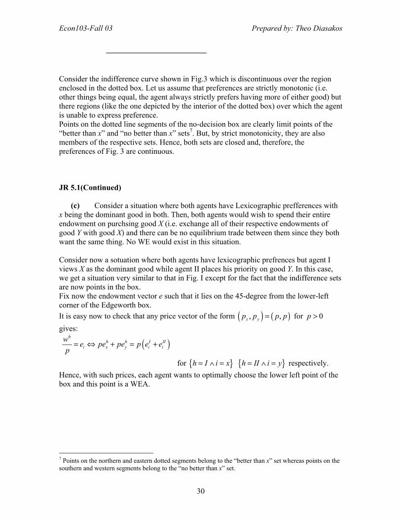
Econ103-Fall 03 Prepared by: Theo Diasakos
1
Problem Set #5 Suggested Solutions
1. Consider the utility contour of agent h i.e. the set of consumption bundles
( ),h h hx a b= that give the same utility level u . This will be given:
( ){ }:h h hx u x u=
Since the utility remains constant at the given level u along the contour, if we totally
differentiate the utility function with respect to the vector hx , we will get:
( ) 0
0
h h
h hh h
h h
h
h h
hh
h
du x du
u uda dba b
udb a
udab
= = ⇔
∂ ∂+ = ⇔∂ ∂
∂∂= −∂∂
This is the slope of the utility contour, at the given point hx , in a ( ),h ha b space. We call
the negative of this slope the Marginal Rate of Substitution (MRS) between ha and hb
at the point hx .
,
h
hh hh aa b hh h
bu uh
uMUdb aMRS
uda MUb
=
∂∂= − = =∂∂
(I)
Note that this gives, by definition, the rate at which agent h is willing to trade between
the goods a and b in order to maintain his level of utility constant at u . Clearly, from (I),
he can do so by exchanging 1unit of good b for hahb
MUMU
units of a.
Econ103-Fall 03 Prepared by: Theo Diasakos
2
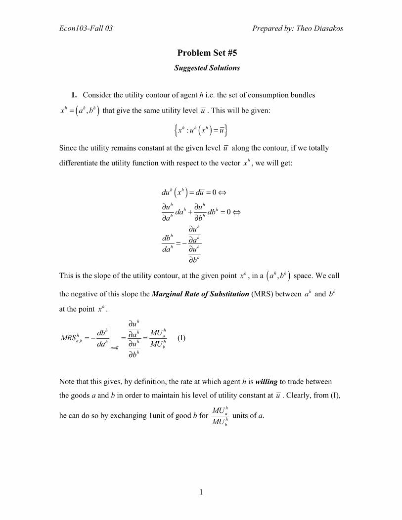
In the given problem, for 1h = , we get: ( )
1
11 11 1
, 1 11 1 1
1
1aa b
bu u
uMUdb aMRS b
uda MU bb
−=
∂∂= − = = = =∂∂
Taking the agent�s consumption set to be 1 2X R+= , we can draw this MRS as an
horizontal line in the ( )1 1,a b space - i.e. it is constant for a given value of 1b ,
independent of the value of 1a (see Fig. I).
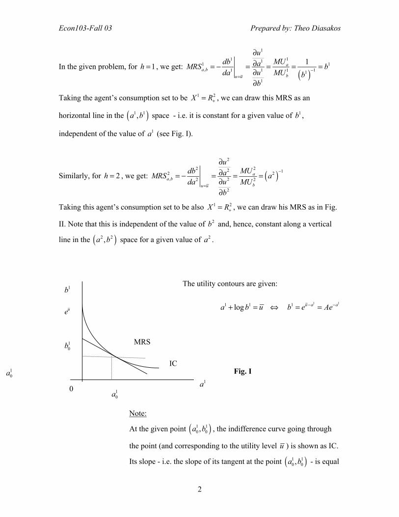
Similarly, for 2h = , we get: ( )2
22 2 12 2, 22 2
2
aa b
bu u
uMUdb aMRS a
uda MUb
−
=
∂∂= − = = =∂∂
Taking this agent�s consumption set to be also 1 2X R+= , we can draw his MRS as in Fig.
II. Note that this is independent of the value of 2b and, hence, constant along a vertical
line in the ( )2 2,a b space for a given value of 2a .
The utility contours are given:
1 11 1 1log u a aa b u b e Ae− −+ = ⇔ = =
Note:
At the given point ( )1 10 0,a b , the indifference curve going through
the point (and corresponding to the utility level u ) is shown as IC.
Its slope - i.e. the slope of its tangent at the point ( )1 10 0,a b - is equal
1b
1a0
Fig. IIC
ue
10b
10a
10a
MRS
Econ103-Fall 03 Prepared by: Theo Diasakos
3
to 10b− . Moreover, if we move along the depicted IC, the slope of
the contour changes according to the equation 1
1 11
u u
db MRS bda =
= − = −
The utility contours are given:
2 2 2 2log loga b u b a u+ = ⇔ = − +
Note:
At the given point ( )2 20 0,a b , the indifference curve going through
the point (and corresponding to the utility level u ) is shown as IC.
Its slope is equal to 201/ a− . Moreover, if we move along the
depicted IC, the slope of the contour changes according to the
equation ( )2 12 22
u u
db MRS ada
−
=
= − = −
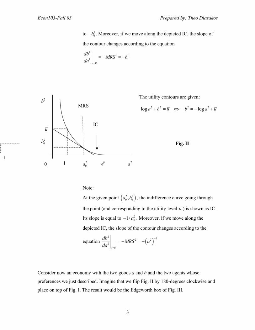
Consider now an economy with the two goods a and b and the two agents whose
preferences we just described. Imagine that we flip Fig. II by 180-degrees clockwise and
place on top of Fig. I. The result would be the Edgeworth box of Fig. III.
2b
2a0
Fig. II
IC
ue
20b
20a
1
u
1
MRS
Econ103-Fall 03 Prepared by: Theo Diasakos
4
Digression on the vary basics of Walrasian Equilibrium Analysis Consider an exchange economy with H consumers, indexed by { }1,...,h H∈ , and N
commodities, indexed by { }1,...,i N∈ . Let us start with a given endowment e, depicted
by an N H× matrix where the element of the i-th row and h-th column will be denoted
by ,h
i m iN He e
× = and taken to mean the quantity of the i-th commodity that the h-th
agent is endowed with.
In this economy, a Walrasian Equilibrium is a price vector ( )
[ ] 11
Ni i
Np p
=×
= and an
allocation matrix ,� �hi m iN H
x x×
= such that:
1a
1b
2a
2b
IC1IC2
Fig. IIIe
1
2
�tan pp
θ =

Econ103-Fall 03 Prepared by: Theo Diasakos
5
1. For each agent, taking the price vector as given, the h-th column of ,�i m N Hx
× -
depicted by the vector ( ) 11� �
Nh hi iN
x x=×
= - solves the following utility maximization
problem:
( )maxh
h h
xU x
s.t. 1 1
N Nh h h h
i i i ii i
px pe p x p e= =
≤ ⇔ ≤∑ ∑
2. The allocation is feasible under exchange of the given endowment. In other
words:
{ }
{ }1 1
1,...,
1,...,
i i
H Hh hi i
h h
x e x e i N
x e i N= =
= ⇔ = ∀ ∈
⇔ = ∀ ∈∑ ∑
Consider now agent h solving his optimization problem.
The Lagrangean function can be written as:
( ) ( ) ( ) ( )1 1 1 1 11 1
,..., ; , ,..., ,..., 0 ... 0N N
h h h h h h h h h h h hN N N i i i i N N
i iL x x U x x p e p x x xλ µ µ λ µ µ
= =
= + − + − + + − ∑ ∑
The first order conditions would be: Set (I)
( ) { }0 1,...,h h
h hi ih h
i i
U xL p i Nx x
λ µ∂∂ = ⇔ = − ∀ ∈
∂ ∂(1)
Set (II)
1 10
H Hh h
i i i ihi i
L p x p eλ = =
∂ ≥ ⇔ ≤∂ ∑ ∑ (2.1)
0hλ ≥ (2.2)

Econ103-Fall 03 Prepared by: Theo Diasakos
6
1 1
0 0H H
h h h hi i i ih
i i
L p e p xλ λλ = =
∂ = ⇔ − = ∂ ∑ ∑ (2.3)
0 0hih
i
L xµ∂ ≥ ⇔ ≥
∂ { }1,...,i N∀ ∈ (3.1)
0hiµ ≥ { }1,...,i N∀ ∈ (3.2)
0 0h h hi i ih
i
L xµ µµ∂ = ⇔ =
∂ { }1,...,i N∀ ∈ (3.3)
Let us assume that (a) we will consider only interior solutions for this optimization
problem (i.e. that the agent chooses to consume � 0hix > { }1,...,i N∀ ∈ ) and (b) the agent
is not satiated with respect to at least one commodity (i.e. there exist commodity, say
{ }1,...,j N∈ , for which 0h
hj j
j
UMU x Rx +
∂= > ∀ ∈∂
).
Then, it is clear from assumption (a) that 0hiµ = { }1,...,i N∀ ∈ .
Hence, the N equations embedded in (1) become:
( ) { }1,...,h h
hih
i
U xp i N
xλ
∂= ∀ ∈
∂ (1.i)
Moreover, by assumption (b), if the price vector is strictly positive
(i.e. 0 0ip p>> ⇔ > { }1,...,i N∀ ∈ ), we conclude that 0hλ > at the optimal point.
Consider now equation (1) across two different commodities. Let us take commodities i
and j. We have:
( )
( )
( )
( ) ,
h h h hh
ih hi hi i i
i jh hh hj jh
hjhjj
U x U xpx x p pMRS
p pU xU xp
xx
λ
λ
∂ ∂=
∂ ∂⇒ = ⇔ =
∂∂ = ∂∂
(I)
Let us now return to our economy as a whole. Looking at the optimization problem of
each of the H agents, it becomes obvious, once we notice that all agents face the same
Econ103-Fall 03 Prepared by: Theo Diasakos
7
price vector p, that all agents� marginal rates of substitution must be the same across a
given pair of commodities. In other words,
, ,h hii j i j
j
pMRS MRSp
= = %
for any two agents { }, 1,...,h h H∈% and any two commodities { }, 1,...,i j N∈ .
The Pareto Efficient Allocations In general, an economic outcome is Pareto optimal (or Pareto efficient (PE)) if there is no
alternative feasible outcome that makes every individual in the economy at least as well
off and some individual strictly beter off.
In terms of the Edgeworth box, two-agent, pure exchange setting, we say that an
allocation x is PE if there is no other allocation x% in the box (i.e. feasible) with h hhx x% f
for 1, 2h = and h hhx x% f for some h.
Mathematically, the set of PE allocations in the Edgeworth box are given by the solution
set of the following problem:
( )
( )
1 2 1 21 2
, , ,
1 2
1 1 1 1 1
2 2 2 2 2
max ,
. .
,
h h h h
h h h
x x x x
h h h
h h h h
h h h h
U x x
s t
U x x u
x x e e e
x x e e e
′ ′
′ ′ ′
′ ′
′ ′
≥
+ = + =
+ = + =
By varying the parameters 1 2 1 2, , , ,h h h he e e e u′ ′ of the problem, we can generate the entire set
of PE allocations (the Pareto set (PS)).
Note that by setting up the Lagrangean of this problem and examining the first order
conditions, it is easy to see that, in the interior of the box, if an allocation is PE then the
MRS�s of the two consumers must be equal at that point (i.e. the two indifference curves
must be tangent).
Econ103-Fall 03 Prepared by: Theo Diasakos
8
By the first fundamental theorem of welfare economics,
• WEAs PS⊂
The Contract Curve The contract curve is defined as that part of the Pareto set where both consumers do at
least as well as their initial endowments.
Note that whereas the Pareto set depends only on the agents� preferences (i.e. the shape
of their indifference curves) the contract curve depends also on the particular endowment
point that they start from (i.e. different initial endowment points for the same consumers
will result to different contract curves).
• Contract Curve PS⊂
The reasoning behind examining the concept of the contract curve is that we might expect
any bargaining between the two agents to result in an agreement to trade to some point on
the contract curve since this is the set of points at which both of them do at least as well
as their endowments and for which there is no alternative trade that can make both of
them better off.
Note also that the definition of the contract curve given in the textbook (see JR, pp. 183)
is lacking because it applies only to allocations in the interior of the box. As we will show
below, an allocation on some of the borders of the box can be on the contract curve
without the indifference curves of the two agents being tangent to one another at that
point.
The Core
Econ103-Fall 03 Prepared by: Theo Diasakos
9
A coalition is any non-empty subset of the set of consumers { }1,...,H H= in an
economy.
A coalition S H⊂ improves upon or blocks the feasible allocation ( )1,..., Hx x x=% % % if for
every h S∈ we can find a consumption bundle 0hx ≥ such that:
1 h hhx x h S∀ ∈%f
2 { }1,...,h hi i
h S h Sx e i N
∈ ∈
= ∀ ∈∑ ∑
Note that this definition says that a coalition S can improve upon a feasible allocation x%
if there is some way, by using only the endowments of its members, for the coalition to
come with an aggregate bundle ( )S s
s Sx x
∈= to distribute amongst its members so as to
make each one better off.
A feasible allocation ( )1,..., Hx x x=% % % has the core property if there is no coalition of
agents S H⊂ that blocks it. The core is the set of allocations that have the core property.
• WEAs Core⊂
When we have only two consumers { }1,2H = the core coincides with the contract curve.
With two consumers there can only be three possible coalitions: { } { } { }1 , 2 , 1, 2 . Any
allocations that is not PE will be blocked by the grand coalition { }1, 2 . Any allocation in
the Pareto set but not on the contract curve will be blocked by either { }1 or { }2 (an agent
who is not at least as well off as at his endowment point can simply use his endowment as
the blocking alternative).
With more than two agents, there can also be other blocking collations. However, the fact
that the whole economy will be the grand coalition means that, in general, all allocations
in the core must be PE.
Econ103-Fall 03 Prepared by: Theo Diasakos
10
• Core PS⊂
We could make a similar argument seeking a general relation between the contract curve
and the core. The fact that each agent on his own can always form a coalition, using his
endowment as a blocking bundle, means that, again in general, an allocation that is not on
the contract curve cannot be in the core (since it would be blocked by whoever was not at
least as well off as at his endowment point).
This statement reads mathematically: x Contract Curve x Core∉ ⇒ ∉% %
Taking the contrapositive statement: x Core x Contract Curve∈ ⇒ ∈% %
• Core Contract Curve⊂
Finally, putting all together:
• WEAs Core Contract Curve PS⊂ ⊂ ⊂
1.(Continued) For the given problem at hand, we have { }2, ,H i a b= ∈ .
At the interior of the Edgeworth box, each agent gets allocated strictly positive quantities
of both goods. Hence, we are looking at an interior solution for both agents. Moreover,
you should verify that assumption (b) is met for both commodities for both agents.
Therefore, at an optimal allocation, both agents would be setting their respective marginal
rates of substitution between the commodities a and b equal to their relative price:
( ) 11 2 1 2 2 1, , 1a
a b a bb
pMRS MRS b a a bp
−= = ⇔ = ⇔ = (II)
However, in the interior of the Edgeworth box, the quantity allocated to each agent of
each commodity being strictly positive means that it is also strictly less than the total
endowment of the commodity (i.e. strictly less than 1 unit in this case)1. But 2 1, 1a b <
1 Clearly, every agent is getting some amount of a given commodity, no one could be getting everything of that commodity.
Econ103-Fall 03 Prepared by: Theo Diasakos
11
cannot satisfy equation (II). Therefore, points in the interior of the box cannot lie on the
contract curve.
Let us now examine the rest of the space of the Edgeworth box � that is, the four border
segments.
It is obvious that agent 1 will never choose to consume zero of commodity b since this
would give him infinitely negative utility. Similarly, agent 2 would never choose to
consume zero of commodity a. Thus, points on the south and east border segments are
out of the question. The same holds, of course, for the southwest, northwest and southeast
corners.
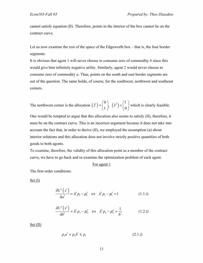
The northwest corner is the allocation ( ) ( )1 20 1� �,
1 0x x
= =
which is clearly feasible.
One would be tempted to argue that this allocation also seems to satisfy (II), therefore, it
must be on the contract curve. This is an incorrect argument because it does not take into
account the fact that, in order to derive (II), we employed the assumption (a) about
interior solutions and this allocation does not involve strictly positive quantities of both
goods to both agents.
To examine, therefore, the validity of this allocation point as a member of the contract
curve, we have to go back and re-examine the optimization problem of each agent.
For agent 1
The first order conditions: Set (I)
( )1 11 1 1 1
1 1 1 11 1U x
p pa
λ µ λ µ∂
= − ⇔ − =∂
(1.1.i)
( )1 1
1 1 1 12 2 2 21 1
1U xp p
b bλ µ λ µ
∂= − ⇔ − =
∂ (1.2.i)
Set (II)
1 11 2 1p a p b p+ ≤ (2.1.i)
Econ103-Fall 03 Prepared by: Theo Diasakos
12
1 0λ ≥ (2.2.i) 1 1 1
1 1 2 0p p a p bλ − − = (2.3.i)
1 0a ≥ 11 0µ ≥ 1 1
1 0aµ = (3.a.i)
1 0b ≥ 12 0µ ≥ 1 1
2 0bµ = (3.b.i)
The consumption bundle ( )1 0�
1x
=
gives: 1 120 0b µ> ⇒ = .
From (1.2.i): 1 12
2
11 0pp
λ λ= ⇔ = >
From (1.1.i): 1 11
2
1pp
µ = −
Note that, for 11 0µ ≥ , we need 1 2p p≥ . This later condition ensures also that (2.1.i) is
satisfied. However, since 1 0λ > , we need to satisfy (2.1.i) with equality, otherwise we would fail (2.3.i). Hence, we really need 1 2p p= .
We conclude, therefore, that if 1 2p p= , then ( )1 0�
1x
=
is a solution to agent�s 1
optimization problem.
For agent 2
The first order conditions: Set (I)
( )2 22 2 2 2
1 1 1 12 2
1U xp p
a aλ µ λ µ
∂= − ⇔ − =
∂ (1.1.ii)
( )2 2
2 2 2 22 2 2 22 1
U xp p
bλ µ λ µ
∂= − ⇔ − =
∂ (1.2.ii)
Set (II)
2 21 2 2p a p b p+ ≤ (2.1.ii)
2 0λ ≥ (2.2.ii)
Econ103-Fall 03 Prepared by: Theo Diasakos
13
2 2 22 1 2 0p p a p bλ − − = (2.3.ii)
2 0a ≥ 21 0µ ≥ 2 2
1 0aµ = (3.a.ii)
2 0b ≥ 22 0µ ≥ 2 2
2 0bµ = (3.b.ii)
The consumption bundle ( )2 1�
0x
=
gives: 2 210 0a µ> ⇒ = .
From (1.1.ii): 2
1
1 0p
λ = >
From (1.2.ii): 2 22
1
1pp
µ = −
Note that, for 22 0µ ≥ , we need 2 1p p≥ . This later condition ensures also that (2.1.ii) is
satisfied. However, since 2 0λ > , we need to satisfy (2.1.ii) with equality, otherwise we would fail (2.3.ii). Hence, we really need 1 2p p= .
We conclude, therefore, that if 1 2p p= , then ( )2 1�
0x
=
is also solution to agent�s 2
optimization problem.
Consequently, for 1 2p p= , the north-west corner allocation ( ) ( )1 20 1� �,
1 0x x
= =
is a
WEA. Therefore, it lies on the contract curve. The Western Border Let us now consider allocations on the western borderline of the Edgeworth box. That is
points of the form ( ) ( )1 2
1 21 2
� �,a a
x xb b
= =
with ( )1 2 1 20, 1, , 0,1a a b b= = ∈
By inspection of the agents� optimization problems we see that we have:
For agent 1, the consumption bundle ( ) ( )1 11
0� : 0,1x b
b
= ∈
gives: 1 120 0b µ> ⇒ = .
From (1.2.i): 11
2
1 0p b
λ = >
From (1.1.i): 1 11 1
2
1pp b
µ = −

Econ103-Fall 03 Prepared by: Theo Diasakos
14
Note that, for 11 0µ ≥ , we need 1
1 2p p b≥ . This later condition ensures also that (2.1.i) is satisfied. However, since 1 0λ > , we need to satisfy (2.1.i) with equality, otherwise we
would fail (2.3.i). Hence, we really need 1 1 11 2
2
pp p b bp
= ⇔ = .
We conclude, therefore, that ( )11 21
2
0� :x p pp
p
= <
is a solution to agent�s 1 optimization
problem that lies on the western border segment of the box.
For agent 2, the consumption bundle ( ) ( )2 22
1� : 0,1x b
b
= ∈
gives: 2 21 2 0µ µ= = .
From (1.2.ii): 2
2
1 0p
λ = >
From (1.2.i): 2
1
1p
λ =
Hence, we require 1 2p p= . But this condition disagrees with (2.1.ii) since it results in 2
2 0p b = - where I have taken also into account the fact that, since 2 0λ > , we need to satisfy (2.2.i) with equality, in the face of (2.3.ii).
We conclude, therefore, that ( ) ( )2 22
1� : 0,1x b
b
= ∈
cannot be a solution to agent�s 2
optimization problem. Note, however, that this point still offers the agent a positive utility level. It is, therefore, preferred to his endowment point.
Hence, the allocation ( ) ( )1 21 21 2 1
2 2
0 1� �, :x x p pp p p
p p
= = <−
is feasible and preferred
by both agents to their respective endowments. It lies, thus, on the contract curve but is not a WEA because it is not optimal for agent II. The Northern Border
Econ103-Fall 03 Prepared by: Theo Diasakos
15
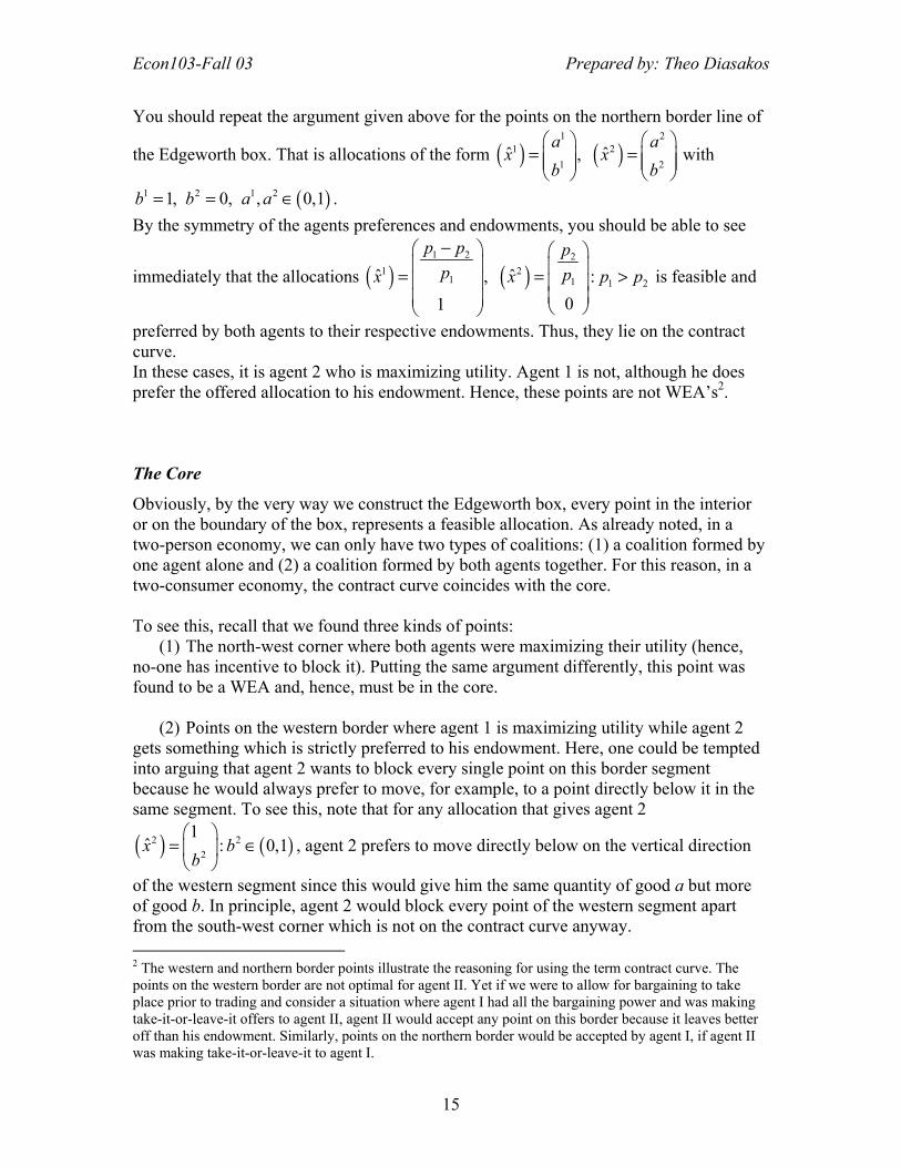
You should repeat the argument given above for the points on the northern border line of
the Edgeworth box. That is allocations of the form ( ) ( )1 2
1 21 2
� �,a a
x xb b
= =
with
( )1 2 1 21, 0, , 0,1b b a a= = ∈ . By the symmetry of the agents preferences and endowments, you should be able to see
immediately that the allocations ( ) ( )1 2 2
1 21 1 1 2� �, :
01
p p pp px x p p−
= = >
is feasible and
preferred by both agents to their respective endowments. Thus, they lie on the contract curve. In these cases, it is agent 2 who is maximizing utility. Agent 1 is not, although he does prefer the offered allocation to his endowment. Hence, these points are not WEA�s2. The Core
Obviously, by the very way we construct the Edgeworth box, every point in the interior or on the boundary of the box, represents a feasible allocation. As already noted, in a two-person economy, we can only have two types of coalitions: (1) a coalition formed by one agent alone and (2) a coalition formed by both agents together. For this reason, in a two-consumer economy, the contract curve coincides with the core. To see this, recall that we found three kinds of points:
(1) The north-west corner where both agents were maximizing their utility (hence, no-one has incentive to block it). Putting the same argument differently, this point was found to be a WEA and, hence, must be in the core.
(2) Points on the western border where agent 1 is maximizing utility while agent 2
gets something which is strictly preferred to his endowment. Here, one could be tempted into arguing that agent 2 wants to block every single point on this border segment because he would always prefer to move, for example, to a point directly below it in the same segment. To see this, note that for any allocation that gives agent 2
( ) ( )2 22
1� : 0,1x b
b
= ∈
, agent 2 prefers to move directly below on the vertical direction
of the western segment since this would give him the same quantity of good a but more of good b. In principle, agent 2 would block every point of the western segment apart from the south-west corner which is not on the contract curve anyway. 2 The western and northern border points illustrate the reasoning for using the term contract curve. The points on the western border are not optimal for agent II. Yet if we were to allow for bargaining to take place prior to trading and consider a situation where agent I had all the bargaining power and was making take-it-or-leave-it offers to agent II, agent II would accept any point on this border because it leaves better off than his endowment. Similarly, points on the northern border would be accepted by agent I, if agent II was making take-it-or-leave-it to agent I.
Econ103-Fall 03 Prepared by: Theo Diasakos
16
This reasoning is flawed, however, because it ignores the requirement in the definition of blocking allocations that the alternative bundle that a coalition offers itself as a blocking device must be generated by the aggregate endowment of the coalition itself (i.e. by re-distributing across coalition members the total endowment of the coalition and of the coalition only). When the coalition consists of a single agent, the only blocking allocation available is his own endowment (since there is no one else in the coalition to switch endowments with).
In our case, therefore, although agent 2 would like to move at points vertically below any given point on the we stern border, he cannot use them as blocking allocations because he cannot offer them to himself using only his endowment.
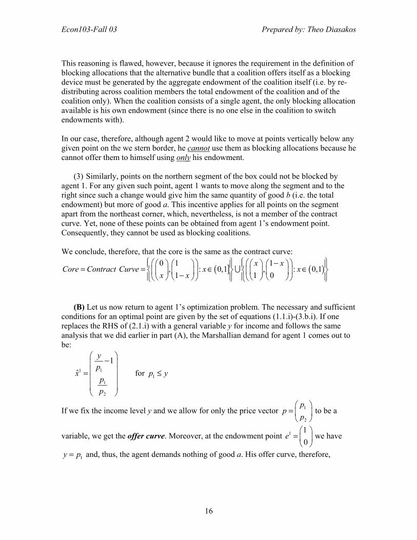
(3) Similarly, points on the northern segment of the box could not be blocked by
agent 1. For any given such point, agent 1 wants to move along the segment and to the right since such a change would give him the same quantity of good b (i.e. the total endowment) but more of good a. This incentive applies for all points on the segment apart from the northeast corner, which, nevertheless, is not a member of the contract curve. Yet, none of these points can be obtained from agent 1�s endowment point. Consequently, they cannot be used as blocking coalitions.
We conclude, therefore, that the core is the same as the contract curve:
( ] ( )0 1 1, : 0,1 , : 0,1
1 1 0x x
Core Contract Curve x xx x
− = = ∈ ∈ − U
(B) Let us now return to agent 1�s optimization problem. The necessary and sufficient
conditions for an optimal point are given by the set of equations (1.1.i)-(3.b.i). If one replaces the RHS of (2.1.i) with a general variable y for income and follows the same analysis that we did earlier in part (A), the Marshallian demand for agent 1 comes out to be:
11
1
2
1�
yp
xpp
− =
for 1p y≤
If we fix the income level y and we allow for only the price vector 1
2
pp
p
=
to be a
variable, we get the offer curve. Moreover, at the endowment point 1 10
e =
we have
1y p= and, thus, the agent demands nothing of good a. His offer curve, therefore,
Econ103-Fall 03 Prepared by: Theo Diasakos
17
becomes 11
2
0x p
p
=
% which is the vertical axis that goes through the given endowment
point. Similarly, for agent 2, we get his Marshallian demand:
2
12
1
�1
pp
xyp
=
−
for 1p y≤
At the endowment point 2 01
e =
we have 2y p= and, thus, the agent demands nothing
of good b. His offer curve, therefore, becomes 2
21
0
ppx
=
% which is the horizontal axis
that goes through the given endowment point.
The two offer curves intersect at the point ( )1 2 0 1, ,
1 0x x
=
for 1 2p p= . We have
already shown that this point, at prices 1 2p p= , is a Walrasian Equilibrium allocation (WEA).
(C) Note first of all that changes in the endowment of agent 1 would correspond to
opposite-direction changes in the endowment of agent 2.
For the Contract Curve: Recall our result that points in the interior of the box cannot lie
on the contract curve (irrespective of the endowment point, since the derivation of the
result did not use the endowment point at all).
Hence, changes in the initial endowment of agent 1 (and accordingly of agent 2) could
only possibly affect the original right-angles contract curve set (recall that this was the
union of the northern and western borders, excluding the upper-right and lower-left
corners). One could think that the contract curve might shrink due to the fact that, by
endowing initially agent 1 with some positive amount of good b, his initial utility level is
no longer negative infinity. Therefore, it should be harder now to maintain points on the
borders as preferred to an endowment point. The same reasoning could be also applied
Econ103-Fall 03 Prepared by: Theo Diasakos
18
from agent 2�s perspective to claim that endowing him with some positive amount of
good a could shrink the contract curve.
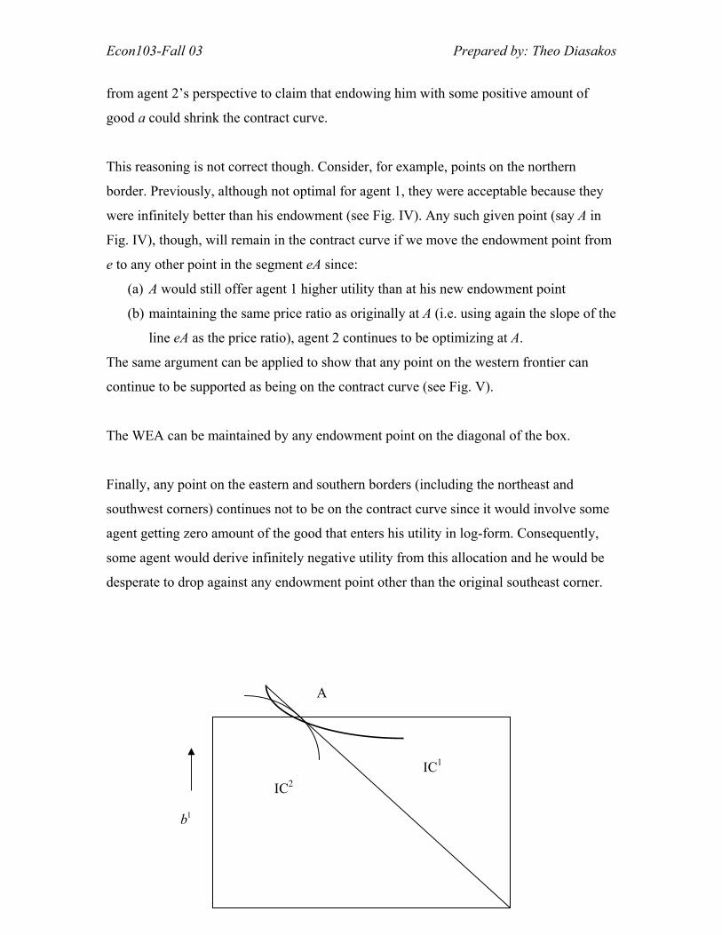
This reasoning is not correct though. Consider, for example, points on the northern
border. Previously, although not optimal for agent 1, they were acceptable because they
were infinitely better than his endowment (see Fig. IV). Any such given point (say A in
Fig. IV), though, will remain in the contract curve if we move the endowment point from
e to any other point in the segment eA since:
(a) A would still offer agent 1 higher utility than at his new endowment point
(b) maintaining the same price ratio as originally at A (i.e. using again the slope of the
line eA as the price ratio), agent 2 continues to be optimizing at A.
The same argument can be applied to show that any point on the western frontier can
continue to be supported as being on the contract curve (see Fig. V).
The WEA can be maintained by any endowment point on the diagonal of the box.
Finally, any point on the eastern and southern borders (including the northeast and
southwest corners) continues not to be on the contract curve since it would involve some
agent getting zero amount of the good that enters his utility in log-form. Consequently,
some agent would derive infinitely negative utility from this allocation and he would be
desperate to drop against any endowment point other than the original southeast corner.
1b
IC1
IC2
A

Econ103-Fall 03 Prepared by: Theo Diasakos
19
For the Offer Curves: In part (B), we found that, in general, the offer curve of agent 1 is
given:
11
1
2
1�
yp
xpp
− =
for 1p y≤
Substituting for 1 11 2a by p e p e= + we get
1 12
11
1
2
1�
a bpe ep
xpp
+ − =
Similar, for agent 2:
1a Fig. IVe
1a
1b IC1
Fig. V e
IC2
Econ103-Fall 03 Prepared by: Theo Diasakos
20
2
12
1
�1
pp
xyp
=
−
for 1p y≤ i.e.
2
12
2 22
1
�1a b
pp
xpe ep
=
+ −
Hence, we see that, changes in the endowment of agent 1 and (correspondingly) agent 2,
other things being equal, would leave unaffected the demands for agent 1 and 2 for goods
b and a respectively.
However, they do affect agent 1�s demand for good a and 2�s demand for good b. The
offer curves for these two commodities are linear in the price ratio with the endowments
determining their slopes and their intercepts. Reducing the endowment of good a for
agent 1 (and, thus, increasing the endowment of agent 2 in this good) will result in a
downward shift of the offer curve of agent 1 for good a and an upward one for the curve
of agent 2 for good b. Similarly, increasing the endowment of good b for agent 1 (and,
thus, decreasing the endowment of agent 2 in this good) will result in making the offer
curve of agent 1 for good a steeper while flattening the curve of agent 2 for good b.
JR 5.12
(a) Consider each agent�s utility maximization problem.
For agent 1, we know that, since his preferences are described by
( ) ( )11 2 1 2, min ,U x x x x=
his optimal bundle will be given by the intersection of the line
1 2x x=
and his budget line
1 1 2 2 1 1 2 2p x p x p e p e+ = + 3
Given his endowment point ( )1 30,0e = we get:
3 Of course, the actual budget constraint is 1 1 2 2 1 1 2 2p x p x p e p e+ ≤ + . However, this agent is non-satiated in either of the two goods. Hence, he will clearly spend all of his income and choose a consumption bundle that lies on the budget line.
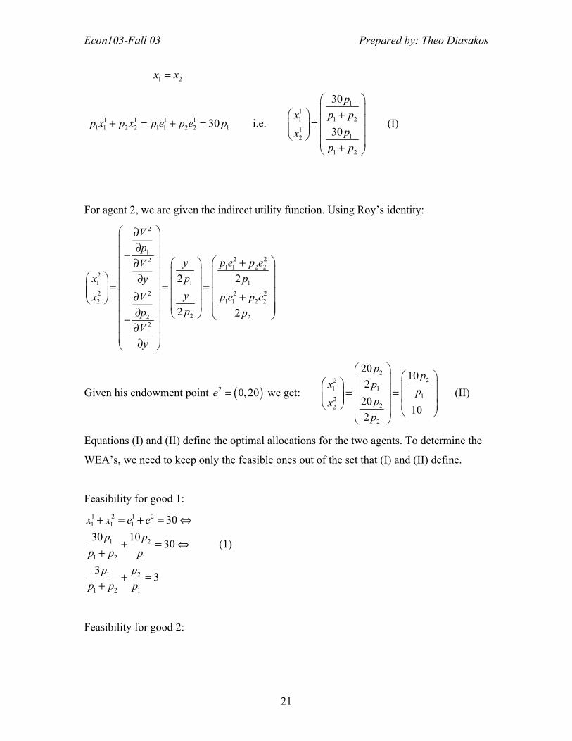
Econ103-Fall 03 Prepared by: Theo Diasakos
21
1 2x x=
1 1 1 11 1 2 2 1 1 2 2 130p x p x p e p e p+ = + = i.e.
111 1 21
12
1 2
30
30
px p p
pxp p
+ = +
(I)
For agent 2, we are given the indirect utility function. Using Roy�s identity: 2
12 22
1 1 2 221 1 12 2 2 22 1 1 2 2
22 22
2 2
2 2
Vp
p e p eyVx p py
yx V p e p epp p
Vy
∂ ∂ −
+∂ ∂ = = = ∂ + ∂ −
∂ ∂
Given his endowment point ( )2 0, 20e = we get:
222
1 112
22
2
20 102
20102
p px p
ppx
p
= =
(II)
Equations (I) and (II) define the optimal allocations for the two agents. To determine the
WEA�s, we need to keep only the feasible ones out of the set that (I) and (II) define.
Feasibility for good 1: 1 2 1 21 1 1 1
1 2
1 2 1
1 2
1 2 1
3030 10 30
3 3
x x e ep p
p p pp p
p p p
+ = + = ⇔
+ = ⇔+
+ =+
(1)
Feasibility for good 2:
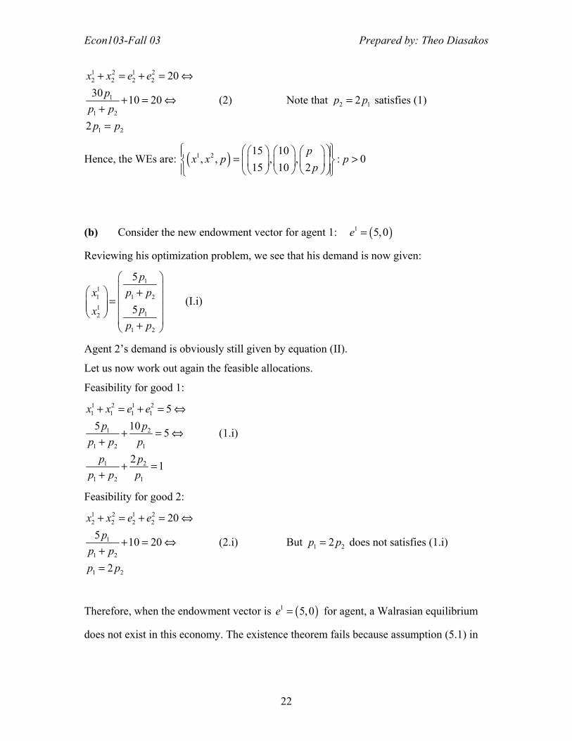
Econ103-Fall 03 Prepared by: Theo Diasakos
22
1 2 1 22 2 2 2
1
1 2
1 2
2030 10 20
2
x x e ep
p pp p
+ = + = ⇔
+ = ⇔+=
(2) Note that 2 12p p= satisfies (1)
Hence, the WEs are: ( )1 2 15 10, , , , : 0
15 10 2p
x x p pp
= >
(b) Consider the new endowment vector for agent 1: ( )1 5,0e =
Reviewing his optimization problem, we see that his demand is now given:
111 1 21
12
1 2
5
5
px p p
pxp p
+ = +
(I.i)
Agent 2�s demand is obviously still given by equation (II).
Let us now work out again the feasible allocations.
Feasibility for good 1: 1 2 1 21 1 1 1
1 2
1 2 1
1 2
1 2 1
55 10 5
2 1
x x e ep p
p p pp p
p p p
+ = + = ⇔
+ = ⇔+
+ =+
(1.i)
Feasibility for good 2: 1 2 1 22 2 2 2
1
1 2
1 2
205 10 20
2
x x e ep
p pp p
+ = + = ⇔
+ = ⇔+=
(2.i) But 1 22p p= does not satisfies (1.i)
Therefore, when the endowment vector is ( )1 5,0e = for agent, a Walrasian equilibrium
does not exist in this economy. The existence theorem fails because assumption (5.1) in
Econ103-Fall 03 Prepared by: Theo Diasakos
23
JR (pp. 188) is not met in this setting since the utility function of agent 1 is not strongly
increasing on 2R+ .
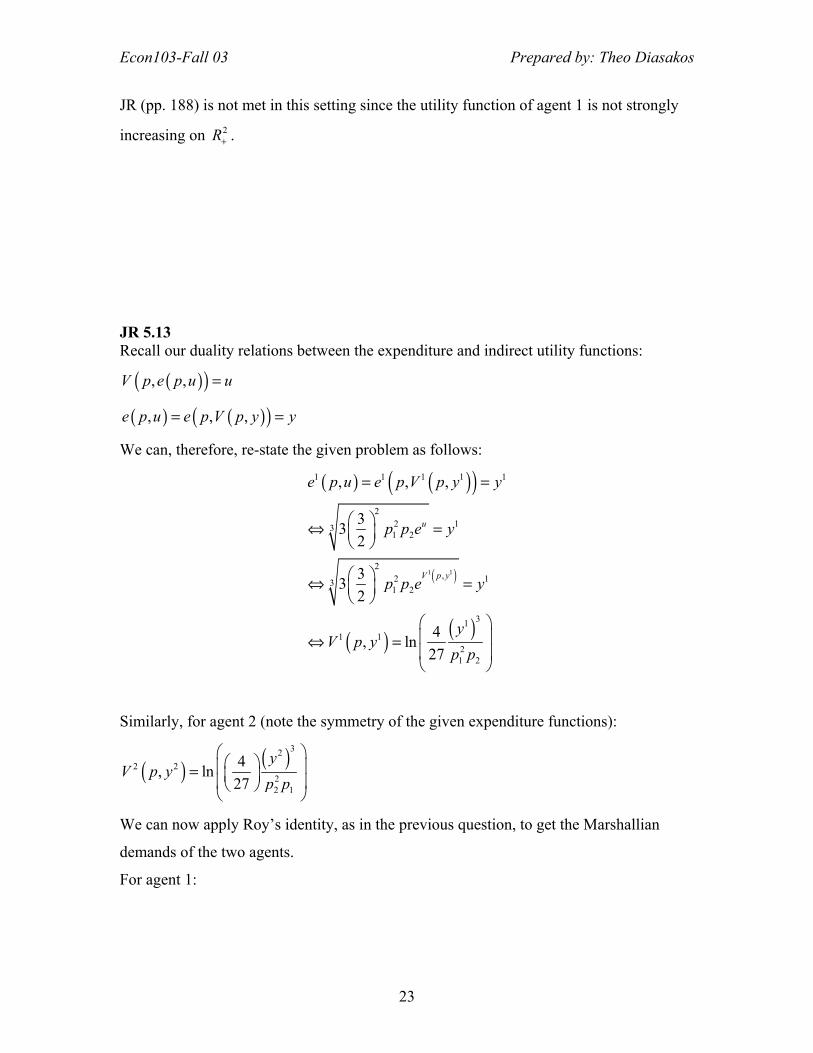
JR 5.13 Recall our duality relations between the expenditure and indirect utility functions:
( )( ), ,V p e p u u=
( ) ( )( ), , ,e p u e p V p y y= =
We can, therefore, re-state the given problem as follows:
( ) ( )( )
( )
( ) ( )
1 1
1 1 1 1 1
22 131 2
2,2 13
1 2
311 1
21 2
, , ,
332
332
4, ln27
u
V p y
e p u e p V p y y
p p e y
p p e y
yV p y
p p
= =
⇔ =
⇔ =
⇔ =
Similarly, for agent 2 (note the symmetry of the given expenditure functions):
( ) ( )322 2
22 1
4, ln27
yV p y
p p
=
We can now apply Roy�s identity, as in the previous question, to get the Marshallian
demands of the two agents.
For agent 1:
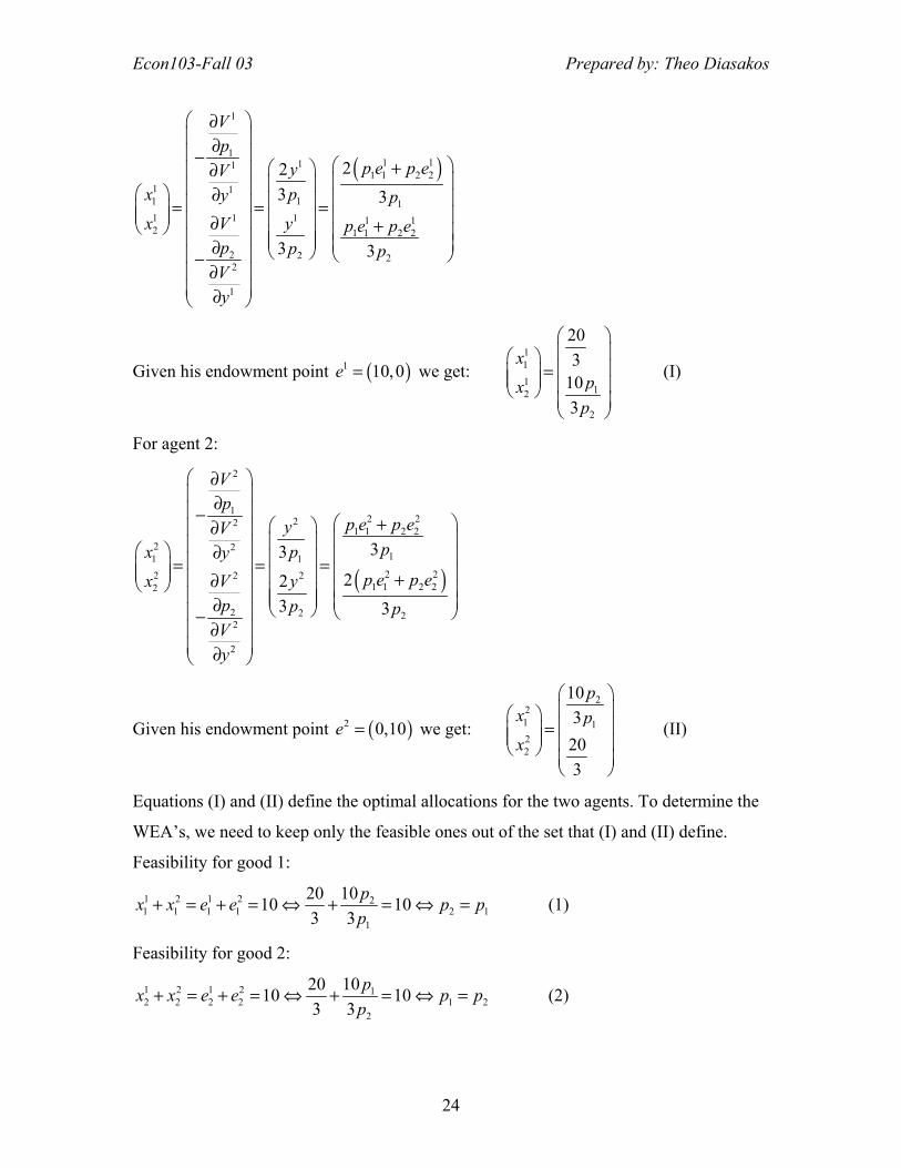
Econ103-Fall 03 Prepared by: Theo Diasakos
24
( )
1
11 111
1 1 2 21 11 1 11 1 1 1 12 1 1 2 2
2 2 22
1
223 3
3 3
Vp
p e p eyVx py px V y p e p e
p p pVy
∂ ∂ − + ∂
∂ = = = ∂ + ∂ − ∂ ∂
Given his endowment point ( )1 10,0e = we get: 111
12
2
203
103
xpx
p
=
(I)
For agent 2:
( )
2
12 222
1 1 2 22 2
11 12 22 2 2
1 1 2 22
2 2 22
2
3322
3 3
Vp
p e p eyVpx py
p e p ex V yp p pVy
∂ ∂ − + ∂
∂ = = = +∂ ∂ − ∂ ∂
Given his endowment point ( )2 0,10e = we get:
221 122
103203
px px
=
(II)
Equations (I) and (II) define the optimal allocations for the two agents. To determine the
WEA�s, we need to keep only the feasible ones out of the set that (I) and (II) define.
Feasibility for good 1:
1 2 1 2 21 1 1 1 2 1
1
102010 103 3
px x e e p pp
+ = + = ⇔ + = ⇔ = (1)
Feasibility for good 2:
1 2 1 2 12 2 2 2 1 2
2
102010 103 3
px x e e p pp
+ = + = ⇔ + = ⇔ = (2)
Econ103-Fall 03 Prepared by: Theo Diasakos
25
Hence, the WEs are: ( )1 2
20 103 3, , , , : 0
10 203 3
px x p p
p
= >
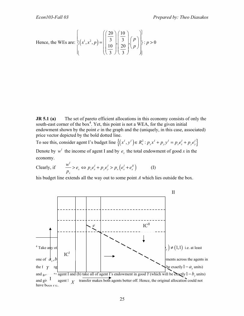
JR 5.1 (a) The set of pareto efficient allocations in this economy consists of only the south-east corner of the box4. Yet, this point is not a WEA, for the given initial endowment shown by the point e in the graph and the (uniquely, in this case, associated) price vector depicted by the bold dotted line. To see this, consider agent I�s budget line ( ){ }2, :I I I I I I
x y x x y yx y R p x p y p e p e+∈ + = +
Denote by Iw the income of agent I and by xe the total endowment of good x in the economy.
Clearly, if ( )I
I I I IIx x x y y x x x
x
w e p e p e p e ep
> ⇔ + > + (I)
his budget line extends all the way out to some point A which lies outside the box.
4 Take any other point of the box - say ( ), , xx
yx
baa b
ba
= such that ( ) ( ), 1,1x ya b ≠ i.e. at least
one of ,x ya b is less than 1. Take that 1xa < . Consider now transferring endowments across the agents in
the following manner: (a) take all of agent II�s endowment in good X (which will be exactly1 xa− units)
and give it to agent I and (b) take all of agent I�s endowment in good Y (which will be exactly1 yb− units) and give it to agent I. This transfer makes both agents better off. Hence, the original allocation could not have been PE. X
Y
I
II
e
ICI
ICII
Econ103-Fall 03 Prepared by: Theo Diasakos
26
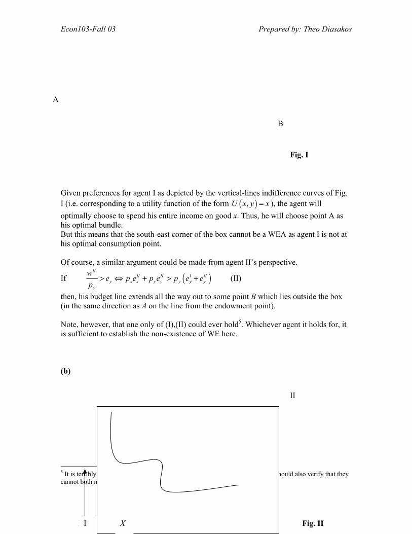
Given preferences for agent I as depicted by the vertical-lines indifference curves of Fig. I (i.e. corresponding to a utility function of the form ( ),U x y x= ), the agent will optimally choose to spend his entire income on good x. Thus, he will choose point A as his optimal bundle. But this means that the south-east corner of the box cannot be a WEA as agent I is not at his optimal consumption point. Of course, a similar argument could be made from agent II�s perspective.
If ( )II
II II I IIy x x y y y y y
y
w e p e p e p e ep
> ⇔ + > + (II)
then, his budget line extends all the way out to some point B which lies outside the box (in the same direction as A on the line from the endowment point). Note, however, that one only of (I),(II) could ever hold5. Whichever agent it holds for, it is sufficient to establish the non-existence of WE here. (b)
5 It is terribly easy to verify that if one of (I),(II) holds, the other must not. You should also verify that they cannot both not hold unless they do so with the negation being equality for both.
II
Fig. I
A
B
X Y I Fig. II

Econ103-Fall 03 Prepared by: Theo Diasakos
27
Digression on Continuity of Preferences Definition of Continuity (version I)6: For all x X∈ , the upper contour set of 0x : { }
0 0:xUC x X x x= ∈ f and the lower contour
set: { }0 0:xLC x X x x= ∈ f are closed in X.
The above is the general definition of continuity for preferences. However, often textbooks use also the following definition as equivalent: Definition of Continuity (version II): The preference relation f on X is continuous if it is preserved under limits. That is, for
any sequence of pairs of bundles ( ){ }1
,n n
nx y
∞
= with n nx y n∀f such that
nnx x
→∞→ and
nny y
→∞→ , we have x yf .
Note that, strictly speaking, the two are not equivalent unless X is a metrizable space. Generally, for X being any topological space, the second version implies continuity under the first (i.e. the second version is sufficient for the general definition) but the sequence definition of continuity is valid only for metrizable spaces. In most applications, we take the consumption space to be some subset of nR which is metrizable (indeed we assume the standard topology using the Euclidean distance metric) and therefore we do not need to worry about the fine print here.
6 In JR (see axiom 3, pp. 8) the upper and lower contour sets are called �at least as good as� set and �no better than� set respectively. Moreover, the consumption set X is taken to be nR+ . I am giving the general
definition of continuity here but will also be using nR+ as the consumption set shortly for graphical representations.
e
ICI
ICII
Econ103-Fall 03 Prepared by: Theo Diasakos
28
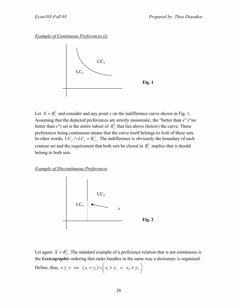
Example of Continuous Preferences (i) Let 2X R+= and consider and any point x on the indifference curve shown in Fig. 1. Assuming that the depicted preferences are strictly monotonic, the �better than x� (�no better than x�) set is the entire subset of 2R+ that lies above (below) the curve. These preferences being continuous means that the curve itself belongs to both of these sets. In other words, x x xUC LC IC∩ = . The indifference is obviously the boundary of each contour set and the requirement that both sets be closed in 2R+ implies that it should belong to both sets. Example of Discontinuous Preferences
Let again 2X R+= . The standard example of a preference relation that is not continuous is the Lexicographic ordering that ranks bundles in the same way a dictionary is organized.
Define, thus, ( )1 1 1 1 2 2x y x y x y x y ⇔ = ∨ > ∧ >
f
UCx
LCx
Fig. 1
UCx
LCx
Fig. 2
x
Econ103-Fall 03 Prepared by: Theo Diasakos
29
In words, commodity 1 has the highest priority in determining the preference ordering just as the first letter word does in the ordering of a dictionary. When the consumption level of the first commodity is the same across two bundles, the amount of the second commodity determines then the preference ranking just as, in the case of the words having the same first letter, we compare the second letters for the dictionary ordering. Consider the indifference sets for this preference relation. It is easy to see that they are singleton, point-sets. Every point x in 2R+ forms a contour set (i.e. any other point in 2R+ will be either better or worse than x). Fig. 2 depicts such a point x. The �better than x� consists of all those points in 2R+ that lie to the right of the vertical axis that goes through the point x including only the solid segment of the axis. Algebraically, this is the set
( ) ( ){ }21 1 2 1 1 2 2:x R x x x R x x x x+ +∈ > ∧ ∈ ∨ = ∧ >% % % % % .
The �better than x� set is not closed in 2R+ because any point in the dotted segment of the
vertical axis that goes through x (i.e. any point in { }21 1 2 2:x R x x x x+∈ = ∧ <% % % ) is a limit
point of this set, yet it does belong in it. Clearly, the �no better than x� set which consists of all points in 2R+ that lie to the left of the vertical axis that goes through x including the dotted segment of the axis, is not closed either. The points that lie on the solid segment of the vertical axis that goes through x are limit points of the �no better than x� set but do not belong in the set itself. Algebraically, the discontinuity of preferences can be easily shown here using version II of the definition of continuity given above. Consider the following sequences of bundles:
( ){ }1 2 1 21
1, : 1 , 0n n n n
nx x x x
n∞
== + = and ( ){ }1 2 1 21
, : 1, 1n n n n
ny y y y
∞
== =
We have:
( ) ( )1 2 1 2, ,n n n nx x y y n Z+∀ ∈f ( ) ( )1 2, 1,0n
n nx x→∞→ but ( ) ( )1,0 1,1p
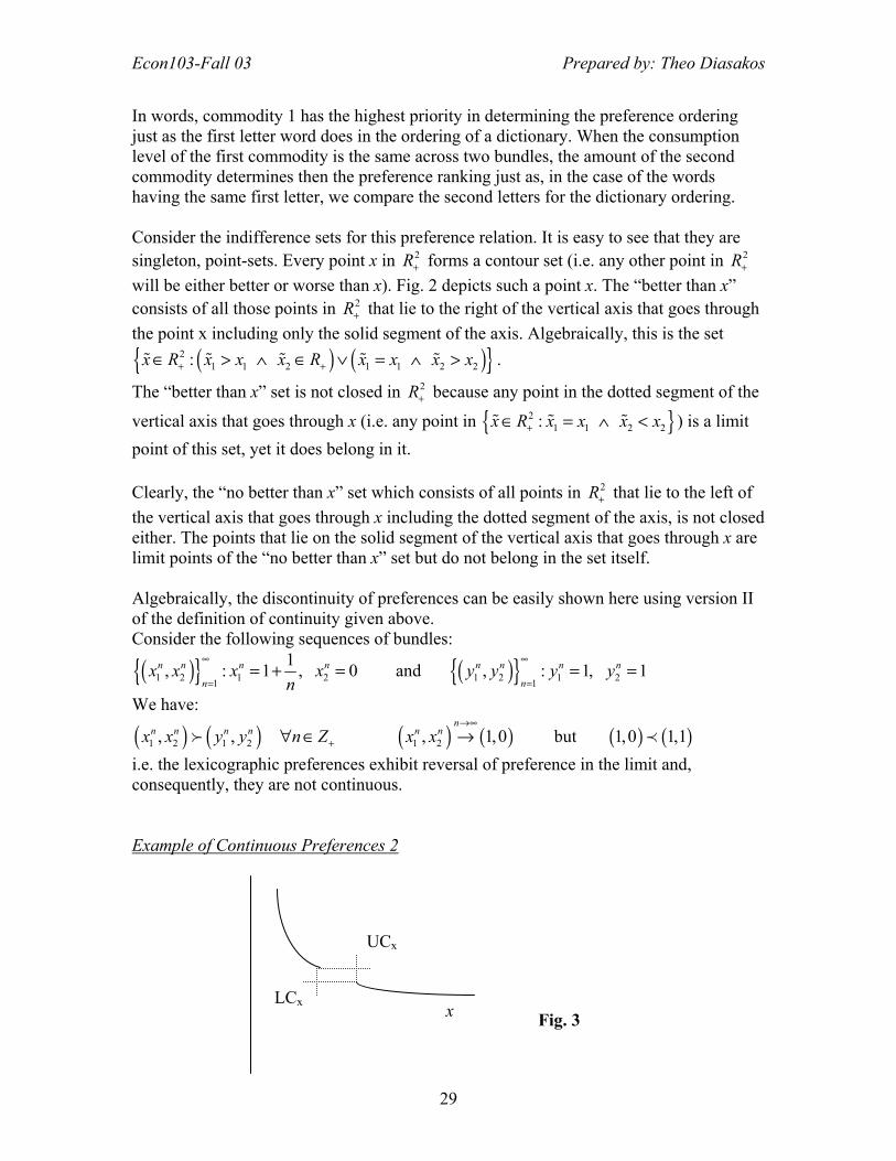
i.e. the lexicographic preferences exhibit reversal of preference in the limit and, consequently, they are not continuous. Example of Continuous Preferences 2
UCx
LCx
Fig. 3 x
Econ103-Fall 03 Prepared by: Theo Diasakos
30
Consider the indifference curve shown in Fig.3 which is discontinuous over the region enclosed in the dotted box. Let us assume that preferences are strictly monotonic (i.e. other things being equal, the agent always strictly prefers having more of either good) but there regions (like the one depicted by the interior of the dotted box) over which the agent is unable to express preference. Points on the dotted line segments of the no-decision box are clearly limit points of the �better than x� and �no better than x� sets7. But, by strict monotonicity, they are also members of the respective sets. Hence, both sets are closed and, therefore, the preferences of Fig. 3 are continuous. JR 5.1(Continued)
(c) Consider a situation where both agents have Lexicographic prefferences with x being the dominant good in both. Then, both agents would wish to spend their entire endowment on purchsing good X (i.e. exchange all of their respective endowments of good Y with good X) and there can be no equilibrium trade between them since they both want the same thing. No WE would exist in this situation. Consider now a sotuation where both agents have lexicographic prefrences but agent I views X as the dominant good while agent II places his priority on good Y. In this case, we get a situation very similar to that in Fig. I except for the fact that the indifference sets are now points in the box. Fix now the endowment vector e such that it lies on the 45-degree from the lower-left corner of the Edgeworth box. It is easy now to check that any price vector of the form ( ) ( ), ,x yp p p p= for 0p > gives:
( )h
h h I IIi x y i i
w e pe pe p e ep
= ⇔ + = +
for { } { }h I i x h II i y= ∧ = = ∧ = respectively. Hence, with such prices, each agent wants to optimally choose the lower left point of the box and this point is a WEA.
7 Points on the northern and eastern dotted segments belong to the �better than x� set whereas points on the southern and western segments belong to the �no better than x� set.