1 tracking systems1
TRANSCRIPT

1
Tracking Systems
SOLO HERMELIN
Updated: 12.10.09Run This
http://www.solohermelin.com

2
Tracking SystemsSOLO
Table of Contents
Chi-square Distribution
Innovation in Kalman Filter
Kalman Filter
Linear Gaussian Markov Systems
Recursive Bayesian Estimation
Target Acceleration Models
General Problem
Evaluation of Kalman Filter Consistency
Innovation in Tracking Systems
Terminology
Functional Diagram of a Tracking System
Filtering and Prediction
Target Models as Markov Processes
Estimation for Static Systems
Information Kalman Filter
Target Estimators
Sensors
3
Tracking SystemsSOLO
Table of Contents (continue – 1)
The Cramér-Rao Lower Bound (CRLB) on the Variance of the Estimator
Nonlinear Estimation (Filtering)
Extended Kalman Filter
Additive Gaussian Nonlinear Filter
Gauss – Hermite Quadrature Approximation
Uscented Kalman Filter
Gating and Data Association
Optimal Correlation of Sensor Data with Tracks on
Surveillance Systems (R.G. Sea, Hughes, 1973)
Gating
Nearest-Neighbor Standard Filter
Global Nearest-Neighbor (GNN) Algorithms
Suboptimal Bayesian Algorithm: The PDAF
Non-Additive Non-Gaussian Nonlinear Filter
Nonlinear Estimation Using Particle Filters

4
Tracking SystemsSOLO
Table of Contents (continue – 2)
Track Life Cycle (Initialization, Maintenance & Deletion)
Filters for Maneuvering Target Detection
The Hybrid Model Approach
No Switching Between Models During the Scenario
Switching Between Models During the Scenario
The Interacting Multiple Model (IMM) Algorithm
The IMM-PDAF Algorithm
The IPDAF Algorithm
Multi-Target Tracking (MTT) Systems
Joint Probabilistic Data Association Filter (JPDAF)
Multi-Sensor Estimate
Track-to-Track of Two Sensors, Correlation and Fusion
Issues in Multi – Sensor Data Fusion
References
Multiple Hypothesis Tracking (MHT)
5
General Problem
I
0Ex
0Ey
Iz
Northx
EastyDownz
Px
Py
Pz
Iy
Ix
t
tLong
Lat
0Ez
Ex
Ey
Ez
AV
Target (T)
(object)
Platform (P)
(sensor)
SOLO
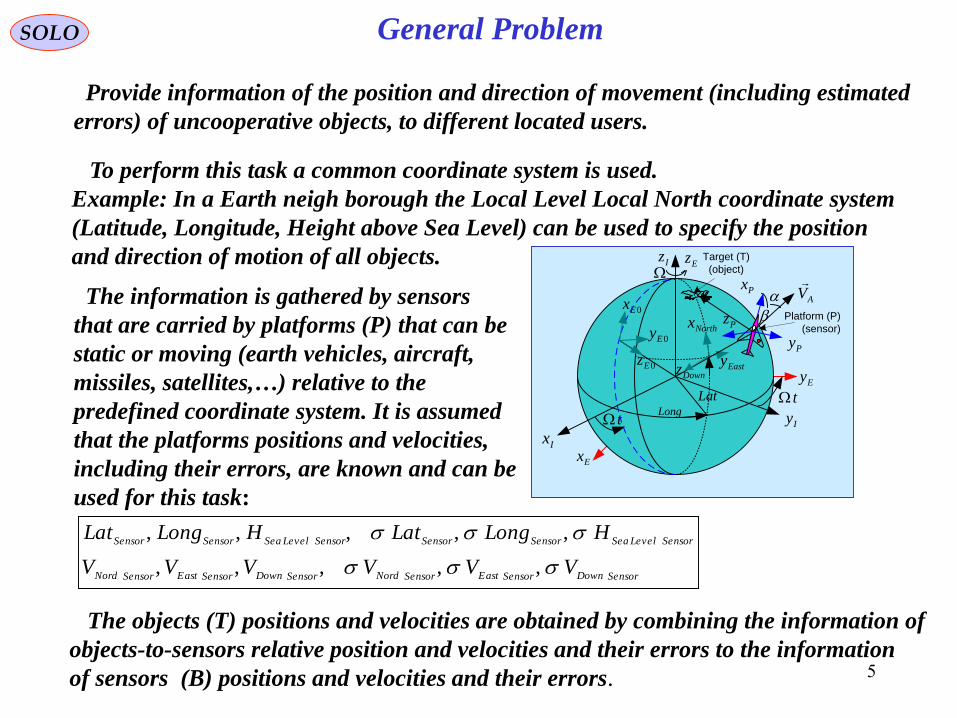
Provide information of the position and direction of movement (including estimated
errors) of uncooperative objects, to different located users.
To perform this task a common coordinate system is used.
Example: In a Earth neigh borough the Local Level Local North coordinate system
(Latitude, Longitude, Height above Sea Level) can be used to specify the position
and direction of motion of all objects.
The information is gathered by sensors
that are carried by platforms (P) that can be
static or moving (earth vehicles, aircraft,
missiles, satellites,…) relative to the
predefined coordinate system. It is assumed
that the platforms positions and velocities,
including their errors, are known and can be
used for this task:
SensorDownSensorEastSensorNordSensorDownSensorEastSensorNord
SensorLevelSeaSensorSensorSensorLevelSeaSensorSensor
VVVVVV
HLongLatHLongLat
,,,,,
,,,,,
The objects (T) positions and velocities are obtained by combining the information of
objects-to-sensors relative position and velocities and their errors to the information
of sensors (B) positions and velocities and their errors.
6
General Problem
Bx
Lx
Bz
Ly
Lz
By
TV
PV
R
Az
El
Bx
SOLO
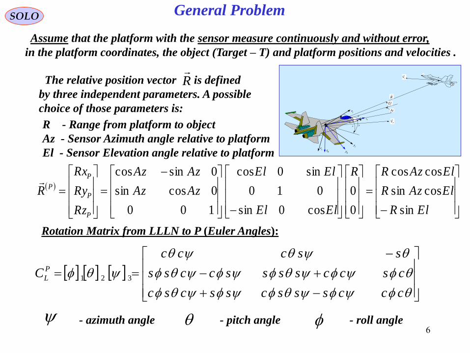
Assume that the platform with the sensor measure continuously and without error,
in the platform coordinates, the object (Target – T) and platform positions and velocities .
The relative position vector is defined
by three independent parameters. A possible
choice of those parameters is:
R
ElR
ElAzR
ElAzRR
ElEl
ElEl
AzAz
AzAz
Rz
Ry
Rx
R
P
P
P
P
sin
cossin
coscos
0
0
cos0sin
010
sin0cos
100
0cossin
0sincos
R - Range from platform to object
Az - Sensor Azimuth angle relative to platform
El - Sensor Elevation angle relative to platform
Rotation Matrix from LLLN to P (Euler Angles):
cccssscsscsc
csccssssccss
ssccc
C P
L 321
- azimuth angle - pitch angle - roll angle

7
General ProblemSOLO
Assume that the platform with the sensor measure continuously and without error,
in the platform coordinates, the object (Target – T) and platform (P) positions and velocities .
The origin of the LLLN coordinate system is located at
the projection of the center of gravity CG of the platform
on the Earth surface, with zDown axis pointed down,
xNorth, yEast plan parallel to the local level, with xNorth
pointed to the local North and yEast pointed to the local East.
The platform is located at:
Latitude = Lat, Longitude = Long, Height = H
Rotation Matrix from E to L
100
0cossin
0sincos
sin0cos
010
cos0sin
2/32 LongLong
LongLong
LatLat
LatLat
LongLatC L
E
LatLongLatLongLat
LongLong
LatLongLatLongLat
sinsincoscoscos
0cossin
cossinsincossin
The earth radius is 26.298/1&10378135.6sin1 6
0
2
0 emRLateRR
pB
The position of the platform in E coordinates is
LongLat
Long
LongLat
HRRBpB
E
B
coscos
sin
cossin
I
0Ex
0Ey
Iz
Northx
EastyDownz
Px
Py
Pz
Iy
Ix
t
tLong
Lat
0Ez
Ex
Ey
Ez
AV
Target (T)
(object)
Platform (P)
(sensor)

8
General Problem
TT
T
TT
TpT
zET
yET
xET
E
T
LongLat
Long
LongLat
HR
R
R
R
R
coscos
sin
cossin
Bx
Lx
Bz
Ly
Lz
By
TV
PV
R
Az
El
Bx
SOLO
The position of the platform (P) in E coordinates is
LongLat
Long
LongLat
HRRBp
E
B
coscos
sin
cossin
The position of the target (T) relative to platform (P)
in E coordinates is
PTP
L
TL
E
PL
P
E
L
E RCCRCCR
The position of the target (T) in E coordinates is
EE
B
zET
yET
xET
E
TRR
R
R
R
R
Since the relation to target latitude LatT, longitude LongT and height HT is given by:
we have
TpTyETT
pTzETyETxETTTpT
zETxETT
HRRLong
RRRRHLateRR
RRLat
/sin
&sin1
/tan
1
2/12222
0
1
Run This
I
0Ex
0Ey
Iz
Northx
EastyDownz
Px
Py
Pz
Iy
Ix
t
tLong
Lat
0Ez
Ex
Ey
Ez
AV
Target (T)
(object)
Platform (P)
(sensor)

9
General Problem
Bx
Lx
Bz
Ly
Lz
By
TV
PV
R
Az
El
Bx
SOLO
Assume that the platform with the sensor measure continuously and without error
in the platform (P) coordinates the object (Target – T) and platform positions and velocities .
Therefore the velocity vector of the object (T)
relative to the platform (P) can be obtained by
direct differentiation of the relative rangeR
PTIP
P
TP VVRtd
RdV
PIP
PI
TT VR
td
Rd
td
RdV
TV
PV
Az
El
Bx
1tR
Time t1
IP
- Angular Rate vector of the
Platform (P) relative to inertia
(measured by its INS)
PV
- Platform (P) Velocity vector
(measured by its INS)
TV
- Target (T) Velocity vector
computed as follows:
TV
PV
2
tR
Az
El
Bx
Bx
Time t2 TV
PV
Az
El
BxBx
Bx
3
tR
Time t3
Ptd
Rd
-Differentiation of vector
in Platform (P) coordinates
R
Run This
10
General Problem
kkx |ˆ
kx
1|1 kkP
1| kkP
1|1ˆ kkx
1kx
kkP |
kkP |1
kkx |1ˆ
kt 1kt
Real Trajectory
Estimated Trajectory
2kt
1|2 kkP
1|2ˆ kkx 2|2 kkP
2|2ˆ kkx
3kt
Measurement Events
Predicted Errors
Updated Errors
SOLO
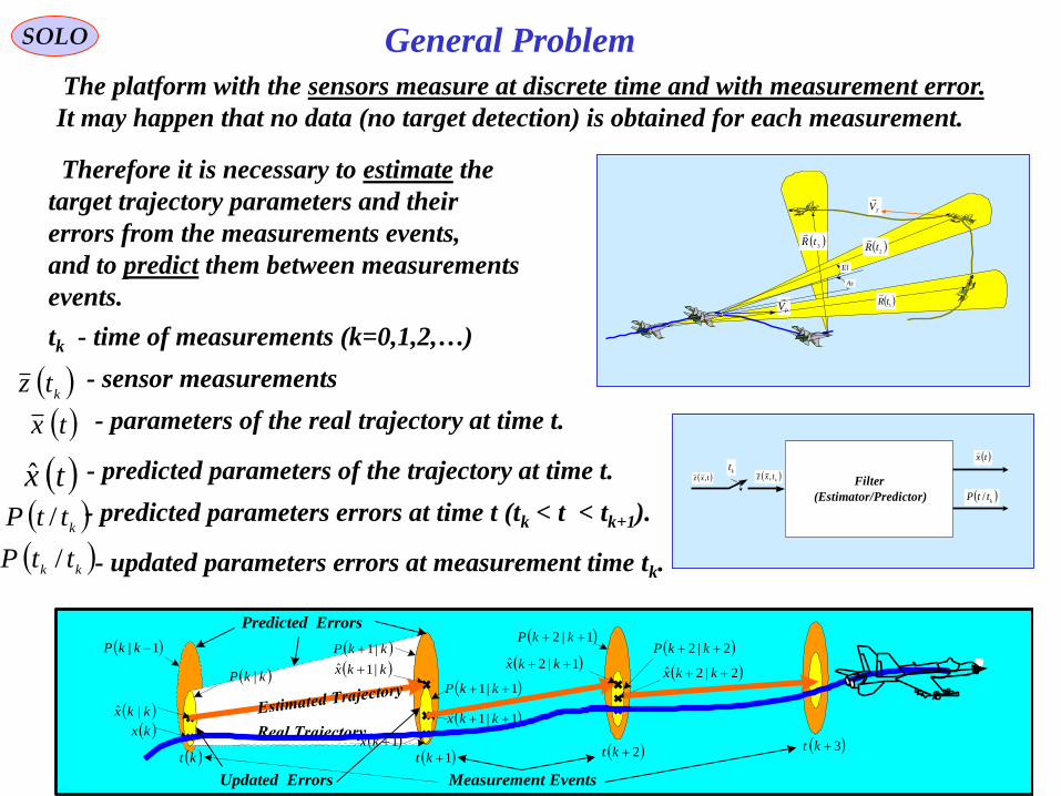
The platform with the sensors measure at discrete time and with measurement error.
It may happen that no data (no target detection) is obtained for each measurement.
Therefore it is necessary to estimate the
target trajectory parameters and their
errors from the measurements events,
and to predict them between measurements
events.
tk - time of measurements (k=0,1,2,…)
- sensor measurements k
tz
- parameters of the real trajectory at time t. tx
- predicted parameters of the trajectory at time t. tx- predicted parameters errors at time t (tk < t < tk+1).
kttP /
- updated parameters errors at measurement time tk. kk
ttP /
txz , Filter
(Estimator/Predictor)
k
txz ,k
t tx
k
ttP /
TV
PV
2
tR
Az
El
Bx
Bx
Bx
1
tR
3
tR
1
1
1

11
General ProblemSOLO
The problem is more complicated when there are Multiple Targets. In this case we must
determinate which measurement is associated to which target. This is done before
filtering.
TV
PV
2
tR
Az
El
Bx
BxB
x
1
tR
3
tR
Bx
Bx
1
2
3
32
1
Bx
Bx
Bx
1
3
2
1
k
txz ,11
k
txz ,22
k
txz ,33
11 | kk ttS
12 | kk ttS
13 | kk ttS
13 |ˆkk ttz
12 |ˆkk ttz
11 |ˆkk ttz
kk ttS |1
kk ttS |2
kk ttS |3
Filter
(Estimator/Predictor)
Target # 1
tx1
k
ttP /1
Filter
(Estimator/Predictor)
Target # N
txN
kN
ttP /
txz , k
txz ,
kt
Data
Association
tz1
tzN
12
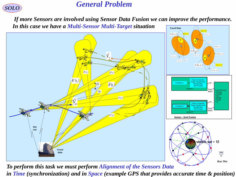
General ProblemSOLO
If more Sensors are involved using Sensor Data Fusion we can improve the performance.
In this case we have a Multi-Sensor Multi-Target situation
1
k
txz ,11
k
txz ,22
k
txz ,33
1
1
1 | kk ttS
1
1
2 | kk ttS
13 | kk ttS
13 |ˆkk ttz
12 |ˆkk ttz
11 |ˆkk ttz
kk ttS |2
3
1st Sensor
1
k
txz ,11
k
txz ,22
k
txz ,33
13 |ˆkk ttz
12 |ˆkk ttz
11 |ˆkk ttz 1
2
1 | kk ttS
1
2
2 | kk ttS
kk ttS |2
3
2nd
Sensor
1
k
txz ,11
k
txz ,22
k
txz ,33
1
1
1 | kk ttS
1
1
2 | kk ttS
13 | kk ttS
13 |ˆkk ttz
12 |ˆkk ttz
11 |ˆkk ttz
kk ttS |1
kk ttS |2
kk ttS |1
3
1
2
1 | kk ttS
1
2
2 | kk ttS
kk ttS |2
3
Fused Data
Transducer 1
Feature Extraction,
Target Classification,
Identification,
and Tracking
Sensor 1Fusion Processor
- Associate
- Correlate
- Track
- Estimate
- Classify
- Cue
Cue
Target
Report
Cue
Target
Report
Sensor – level Fusion
Transducer 2
Feature Extraction,
Target Classification,
Identification,
and Tracking
Sensor 2
1
TV
PV
2
1 tR
Az
El
Bx
Bx
Bx
1
1 tR
3
1 tR
Bx
Bx
2
3
32
1
Bx
Bx
Bx
Bx
1
3
2
1st Sensor
1
TV
PV
Bx
Bx
Bx
Bx
Bx
2
3
32
1
Bx
Bx
Bx
Bx
1
3
2
Ground
Radar
Data
Link
1
2 tR
2
2 tR 3
2 tR
2nd
Sensor
1
TV
PV
2
1 tR
Az
El
Bx
Bx
Bx
1
1 tR
3
1 tR
Bx
Bx
2
3
32
1
Bx
Bx
Bx
Bx
1
3
2
Ground
Radar
Data
Link
1
2 tR
2
2 tR 3
2 tR
To perform this task we must perform Alignment of the Sensors Data
in Time (synchronization) and in Space (example GPS that provides accurate time & position)
Run This
13
General ProblemSOLO
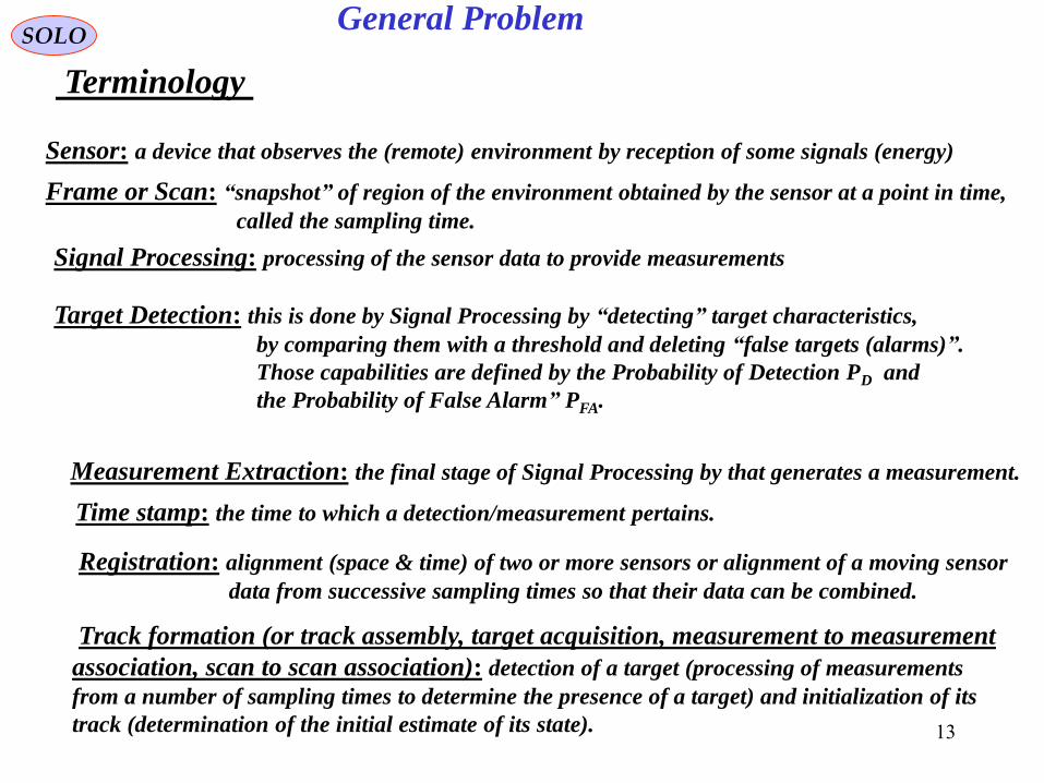
Terminology
Sensor: a device that observes the (remote) environment by reception of some signals (energy)
Frame or Scan: “snapshot” of region of the environment obtained by the sensor at a point in time,
called the sampling time.
Signal Processing: processing of the sensor data to provide measurements
Target Detection: this is done by Signal Processing by “detecting” target characteristics,
by comparing them with a threshold and deleting “false targets (alarms)”.
Those capabilities are defined by the Probability of Detection PD and
the Probability of False Alarm” PFA.
Measurement Extraction: the final stage of Signal Processing by that generates a measurement.
Time stamp: the time to which a detection/measurement pertains.
Registration: alignment (space & time) of two or more sensors or alignment of a moving sensor
data from successive sampling times so that their data can be combined.
Track formation (or track assembly, target acquisition, measurement to measurement
association, scan to scan association): detection of a target (processing of measurements
from a number of sampling times to determine the presence of a target) and initialization of its
track (determination of the initial estimate of its state).

14
General ProblemSOLO
Terminology (continue – 1)
Tracking filter: state estimator of a target.
Data association: process of establishing which measurement (or weighted combination of
measurements) to be used in a state estimator.
Track continuation (maintenance or updating): association and incorporation of
measurements from a sampling time into a track filter.
Cluster tracking tracking of a set of nearby targets as a group rather than individuals.
Return to Table of Content

15
General ProblemSOLO
Return to Table of Content
Sensor Data
Processing and
Measurement
Formation
Observation -
to - Track
Association
Input
DataTrack
Maintenance
(Initialization,
Confirmation
and Deletion)
Filtering and
Prediction
Gating
Computations
Samuel S . Blackman , " Multiple-Target Tracking with Radar Applications ", Artech House ,
1986Samuel S . Blackman , Robert Popoli , " Design and Analysis of Modern Tracking Systems
", Artech House , 1999
Functional Diagram of a Tracking System
A Tracking System performs the following functions:
• Sensors Data Processing and Measurement
Formation that provides Targets Data
• Observation-to-Track Association
that relates Target Detected Data
to Existing Track Files.
• Track Maintenance (Initialization,
Confirmation and Deletion) of the
Targets Detected by the Sensors.
• Filtering and Prediction , for each Track processes the Data Associated to the Track,
Filter the Target State (Position, and may be Velocity and Acceleration) from Noise,
and Predict the Target State and Errors (Covariance Matrix) at the next
Sensors Measurement.
• Gating Computations that, using the Predicted Target State, provides the Gating to
enabling distinguishing between the Measurement from the Target of the specific
Track File to other Targets Detected by the Sensors.

16
SENSORSSOLO
Introduction
Classification of Sensors by the type of energy they use for sensing:
We deal with sensors used for target detection, identification,
acquisition and tracking, seekers for missile guidance.
• Electromagnetic Effect that are distinct by EM frequency:
- Micro-Wave Electro-Optical:
* Visible
* IR
* Laser
- Millimeter Wave Radars
• Acoustic Systems
Classification of Sensors by the source of energy they use for sensing:
• Passive where the source of energy is in the objects that are sensed
Example: Visible, IR, Acoustic Systems
• Semi – Active where the source of energy is actively produced externally to
the Sensor and sent toward the target that reflected it back to the sensor
Example: Radars, Laser, Acoustic Systems
• Active where the source of energy is actively produced by the Sensor
and sent toward the target that reflected it back to the sensor
Example: Radars, Laser, Acoustic Systems
Sensor Data
Processing and
Measurement
Formation
Observation -
to - Track
Association
Input
DataTrack
Maintenance
) Initialization,
Confirmation
and Deletion(
Filtering and
Prediction
Gating
Computations
Samuel S . Blackman , " Multiple-Target Tracking with Radar Applications ", Artech House ,
1986Samuel S . Blackman , Robert Popoli , " Design and Analysis of Modern Tracking Systems
", Artech House , 1999

17
SENSORSSOLO
Introduction
Classification of Sensors by the Carrying Vehicle:
• Sensors on Ground Fixed Sites
• Human Carriers
• Ground Vehicles
• Ships
• Submarines
• Torpedoes
• Air Vehicles (Aircraft, Helicopters, UAV, Balloons)
• Missiles (Seekers, Active Proximity Fuzes)
• Satellites
Classification of Sensors by the Measurements Type:
• Range and Direction to the Target (Active Sensors)
• Direction to the Target only (Passive and Semi-Active Sensors)
• Imaging of the Object
• Non-Imaging
See “Sensors.ppt” for
a detailed description

18
SENSORSSOLO
Introduction
1. Search Phase
Sensor Processes:
In this Phase a search for predefined Targets is performed.
The search is done to cover a predefined (or cued) Space Region.
The Angular Coverage may be performed by
• Scanning (Mechanically/Electronically) the Space Region
(Radar, EO Sensors)
• Steering toward the Space Region (EO Sensors, Sonar)
Radar System can perform also Search in Range and Range-Rate
2. Detection Phase
In this Phase the predefined Target is Detected, extracted from the noise and the
Background using the Target Properties that differentiate it, like:
• Target Intensity (Radar, EO Sensors, Sonars)
• Target Kinematics relative to the Background (Radar, EO Sensors, Sonars)
• Target Shape (EO Sensors, Radar)
The Sensor can use one or a combination of those methods.
There is a Probability that a False Target will be detected, therefore two quantities
Define the Detection performance:
• Probability of Detection ( ≤ 1 )
• Probability of False Alarm
Search
Search
Command
Detect
19
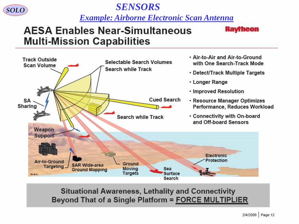
SOLOExample: Airborne Electronic Scan Antenna
SENSORS

20
SENSORSSOLO
Introduction
3. Identification Phase
Sensor Processes (continue – 1):
In this Phase the Target of Interest is differentiate from
other Detected Targets.
4. Acquisition Phase
In this Phase we check that the Detection and Identification
occurred for a number of Search Frames and Initializes the
Track Phase.
5. Track Phase
In this Phase the Sensor, will update the
History of each Target (Track File),
Associating the Data in the present frame
to previous Histories. This phase continues
until Target Detection is not available for
a predefined number of frames.
Search
Search
Command
Detect
Identify
Target
Acquire
TrackReacquire
End-of-Track

2121
SOLO
Properties of Electro-Magnetic Waves
SENSORS

22
SOLO
Generic Airborne Radar Block Diagram
f0
Receiver
REF
XMTR
Digital
Signal
Proc.Radar Central
Computer
Pilot
CommandsData to
Displays
Antenna
Unit
T/R
(Circulator)
Power
Supply
A/D
Digital
Analog
Command &
Control Aircraft
AvionicsAvionics
BUS
Beam Control
(Mechanical or
Electronical)
Aircraft Power
Airborne Radar Block Diagram
Antenna – Transmits and receives Electromagnetic
Energy
T/R – Isolates between transmitting and receiving
channels
REF – Generates and Controls all Radar frequencies
XMTR – Transmits High Power EM Radar frequencies
RECEIVER – Receives Returned Radar Power, filter it
and down-converted to Base Band for
digitization trough A/D.
Digital Signal Processor – Processes all
the digitized signal to enhance the Target
of interest versus all other (clutter).
Power Supply – Supplies Power to all Radar components.
Radar Central Computer – Controls all
Radar Units activities, according to Pilot
Commands and Avionics data, and provides
output to Pilot Displays and Avionics.
SENSORS

23
Table of Content
SOLO

24
Radar Antenna

25
Radar Antenna

26
Radar Antenna

27
Radar Antenna

28
SOLO E-O and IR Systems Payloads
See “E-O & IR Systems
Payloads”.ppt for a detailed
presentation

29
SOLO E-O and IR Systems Payloads
0.9 kg 2.27 kg1.06 kg0.55 kg
Small, lightweight gimbals which come standard with rich features such as built-in moving maps, geo-
pointing and geo-locating. Cloud Cap gimbals are robust and proven with over 300 gimbals sold to date.
Complete with command/control/record software and joystick steering, Cloud Cap gimbals are ideal for
surveillance, inspection, law enforcement, fire fighting, and environmental monitoring. View a
comparison table of specifications for the TASE family of Gimbals.

30
SOLO
RAFAEL LITENING
Multi-Sensor, Multi-Mission Targeting & Navigation Pod
E-O and IR Systems Payloads

31
SOLO
RAFAEL RECCELITE
Real-Time Tactical Reconnaissance System
E-O and IR Systems Payloads

33
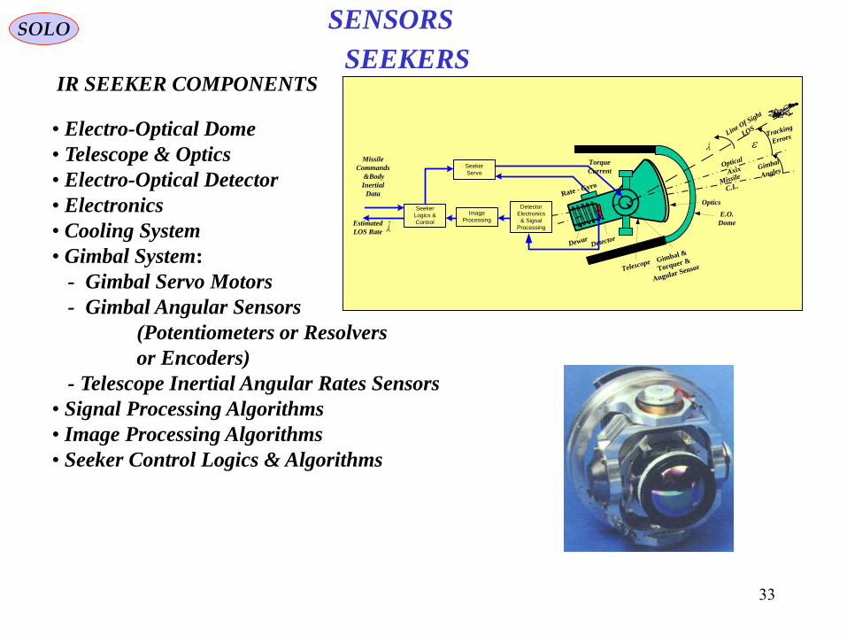
SEEKERS
SOLO
IR SEEKER COMPONENTS
• Electro-Optical Dome
• Telescope & Optics
• Electro-Optical Detector
• Electronics
• Cooling System
• Gimbal System:
- Gimbal Servo Motors
- Gimbal Angular Sensors
(Potentiometers or Resolvers
or Encoders)
- Telescope Inertial Angular Rates Sensors
• Signal Processing Algorithms
• Image Processing Algorithms
• Seeker Control Logics & Algorithms
Detector
Electronics
& Signal
Processing
Image
Processing
Seeker
Servo
Gimbal &
Torquer &
Angular Sensor
E.O.
Dome
Optics
Telescope
DetectorDewar
Optical
Axix
Missile
C.L.
Line Of S
ight
LOS
Estimated
LOS Rate
Seeker
Logics &
Control
Missile
Commands
&Body
Inertial
Data
Gimbal
Angles
Tracking
Errors
Torque
Current
Rate - Gyro
SENSORS
34
Decision/Detection Theory
SOLO
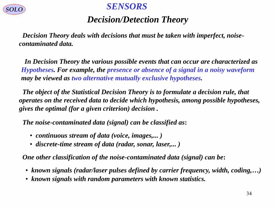
Decision Theory deals with decisions that must be taken with imperfect, noise-
contaminated data.
In Decision Theory the various possible events that can occur are characterized as
Hypotheses. For example, the presence or absence of a signal in a noisy waveform
may be viewed as two alternative mutually exclusive hypotheses.
The object of the Statistical Decision Theory is to formulate a decision rule, that
operates on the received data to decide which hypothesis, among possible hypotheses,
gives the optimal (for a given criterion) decision .
The noise-contaminated data (signal) can be classified as:
• continuous stream of data (voice, images,... )
• discrete-time stream of data (radar, sonar, laser,... )
One other classification of the noise-contaminated data (signal) can be:
• known signals (radar/laser pulses defined by carrier frequency, width, coding,…)
• known signals with random parameters with known statistics.
SENSORS

35
Decision/Detection Theory
SOLO
Hypotheses
H0 – target is not present
H1 – target is present
Binary Detection
0
Hp - probability that target is not present
1
Hp - probability that target is present
zHp |0 - probability that target is not present and not declared (correct decision)
zHp |1 - probability that target is present and declared (correct decision)
Using Bayes’ rule: Z
dzzpzHpHp |00
Z
dzzpzHpHp |11
zp - probability of the event Zz
Since p (z) > 0 the Decision rules are:
zHpzHp ||01
- target is not declared (H0)
zHpzHp ||01
- target is declared (H1) zHpzHp
H
H
||01
0
1
SENSORS

36
Decision/Detection Theory
SOLO
Hypotheses H0 – target is not present H1 – target is present
Binary Detection
zHp |0 - probability that target is not present and not declared (correct decision)
zHp |1 - probability that target is present and declared (correct decision)
zp - probability of the event Zz
Decision rules are: zHpzHp
H
H
||01
0
1
Using again Bayes’ rule:
zp
HpHzpzHp
zp
HpHzpzHp
H
H
00
0
11
1
||
||
0
1
0
| Hzp - a priori probability that target is not present (H0)
1
| Hzp - a priori probability that target is present (H1)
Since all probabilities are
non-negative
1
0
0
1
0
1
|
|
Hp
Hp
Hzp
Hzp
H
H
SENSORS

37
Decision/Detection Theory
SOLO
Hypotheses
1
| Hzp - a priori probability density that target is present (likelihood of H1)
0
| Hzp - a priori probability density that target is absent (likelihood of H0)
PD - probability of detection = probability that the target is present and declared
PFA - probability of false alarm = probability that the target is absent but declared
PM - probability of miss = probability that the target is present but not declared
T - detection threshold
Detection Probabilities
M
z
DPdzHzpP
T
1|1
Tz
FAdzHzpP
0|
D
z
MPdzHzpP
T
1|1
DP
FAP
1
| Hzp 0
| Hzp
MP
z
Tz
THzp
Hzp
T
T 0
1
|
|
H0 – target is not present H1 – target is present
Binary Detection
THp
Hp
Hzp
HzpLR
H
H
1
0
0
1
0
1
|
|:Likelihood Ratio Test (LTR)
SENSORS

38
Decision/Detection TheorySOLO
Hypotheses
Decision Criteria on Definition of the Threshold T
1. Bayes Criterion
DP
FAP
1
| Hzp 0
| Hzp
MP
z
Tz
THzp
Hzp
T
T 0
1
|
|
H0 – target is not present H1 – target is present
Binary Detection
THp
Hp
Hzp
HzpLR
H
H
1
0
0
1
0
1
|
|:Likelihood Ratio Test (LTR)
The optimal choice that optimizes the Likelihood Ratio is
1
0
Hp
HpT
Bayes
This choose assume knowledge of p (H0) and P (H1), that in general are not known a priori.
2. Maximum Likelihood Criterion
Since p (H0) and P (H1) are not known a priori, we choose TML = 1
1
| Hzp 0
| Hzp
MP z
Tz
1|
|
0
1 ML
T
T THzp
Hzp
DP
FAP
SENSORS

39
Decision/Detection Theory
SOLO
Hypotheses
Decision Criteria on Definition of the Threshold T (continue)
3. Neyman-Pearson Criterion
H0 – target is not present H1 – target is present
Binary Detection
THp
Hp
Hzp
HzpLR
H
H
1
0
0
1
0
1
|
|:Likelihood Ratio Test (LTR)
Egon Sharpe Pearson
1895 - 1980
Jerzy Neyman
1894 - 1981
Neyman and Pearson choose to optimizes the probability of detection PD
keeping the probability of false alarm PFA constant.
T
TT
z
zD
zdzHzpP
1|maxmax
Tz
FAdzHzpP
0|constrained to
Let use the Lagrange’s multiplier λ to add the constraint
TT
TT
zz
zzdzHzpdzHzpG
01||maxmax
Maximum is obtained for:
0||01
HzpHzp
z
GTT
T
DP
FA
P
1
| Hzp 0
| Hzp
MP
z
Tz
PN
T
T THzp
Hzp
0
1
|
|
PN
T
T THzp
Hzp
0
1
|
|
zT is define by requiring that:
Tz
FAdzHzpP
0|
SENSORS

40
SOLO
Return to Table of Content
Sensor Data
Processing and
Measurement
Formation
Observation -
to - Track
Association
Input
DataTrack
Maintenance
(Initialization,
Confirmation
and Deletion)
Filtering and
Prediction
Gating
Computations
Samuel S . Blackman , " Multiple-Target Tracking with Radar Applications ", Artech House ,
1986Samuel S . Blackman , Robert Popoli , " Design and Analysis of Modern Tracking Systems
", Artech House , 1999
Filtering and Prediction
• Filtering and Prediction , for each Track processes the Data Associated to the Track,
Filter the Target State (Position, and may be Velocity and Acceleration) from Noise,
and Predict the Target State and Errors (Covariance Matrix) at the next
Sensors Measurement.
kkx |ˆ
kx
1|1 kkP
1| kkP
1|1ˆ kkx
1kx
kkP |
kkP |1
kkx |1ˆ
kt 1kt
Real Trajectory
Estimated Trajectory
2kt
1|2 kkP
1|2ˆ kkx 2|2 kkP
2|2ˆ kkx
3kt
Measurement Events
Predicted Errors
Updated Errors

41
SOLO
Discrete Filter/Predictor Architecture
State at tk
x (k)
Evolution
of the system
(true state)
Transition to tk+1
x (k+1)=
F(k) x (k)
+ G (k) u (k)+ v (k)
Measurement at tk+1
z (k+1)=
H (k) x (k)+ w (k)
Control at tk
u (k)
Controller
kt
1kt
kx
1kx kt 1kt
Real Trajectory
The discrete representation of the system is given by
x (k) - system state vector
kwkxkHkz
kvkukGkxkFkx
111
1
u (k) - system control input
v (k) - system unknown dynamics assumed white Gaussian
w (k) - measurement noise assumed white Gaussian
k - discrete time counter
Filtering and Prediction Sensor Data
Processing and
Measurement
Formation
Observation -
to - Track
Association
Input
DataTrack
Maintenance
(Initialization,
Confirmation
and Deletion)
Filtering and
Prediction
Gating
Computations
Samuel S . Blackman , " Multiple-Target Tracking with Radar Applications ", Artech House ,
1986Samuel S . Blackman , Robert Popoli , " Design and Analysis of Modern Tracking Systems
", Artech House , 1999

42
SOLO
Discrete Filter/Predictor Architecture (continue – 1)
State at tk
x (k)
Evolution
of the system
(true state)
Transition to tk+1
x (k+1)=
F(k) x (k)
+ G (k) u (k)+ v (k)
Measurement at tk+1
z (k+1)=
H (k) x (k)+ w (k)
Control at tk
u (k)
Controller
kt
1kt
kx
1kx kt 1kt
Real Trajectory
1. The output of the Filter/Predictor can
be at a higher rate than the input
(measurements)
Tmeasurements = m Toutput, m integer
2. Between measurements it will perform
State Prediction
kkxkHkkz
kukGkkxkFkkx
|1ˆ1|1ˆ
|ˆ|1ˆ
3. At measurements it will perform
Update State
11|1ˆ|1ˆ
|1ˆ11
kkKkkxkkx
kkxkHkzk
υ (k) - Innovation
K (k) – Filter Gain
State at tk
x (k)
Evolution
of the system
(true state)
Transition to tk+1
x (k+1)=
F(k) x (k)
+ G (k) u (k)+ v (k)
Measurement at tk+1
z (k+1)=
H (k) x (k)+ w (k)
Estimation
of the state
Control at tk
u (k)
Controller
State Prediction
at tk +1
kukGkkxkF
kkx
|ˆ
|1ˆ
Measurement
Prediction
at tk +1
kkxkHkkz |1ˆ1|1ˆ
Innovation
kkzkzkv |1ˆ11
Update State
Estimation at tk +1
11|1ˆ
1|1ˆ
kvkKkkx
kkx
kt
1kt
State
Estimation
at tk
kkx |ˆ
kkx |ˆ
kx 1|1ˆ kkx
1kx
kkx |1ˆ
kt 1kt
Real Trajectory
Estimated
Trajectory
1kK
Filtering and PredictionSensor Data
Processing and
Measurement
Formation
Observation -
to - Track
Association
Input
DataTrack
Maintenance
(Initialization,
Confirmation
and Deletion)
Filtering and
Prediction
Gating
Computations
Samuel S . Blackman , " Multiple-Target Tracking with Radar Applications ", Artech House ,
1986Samuel S . Blackman , Robert Popoli , " Design and Analysis of Modern Tracking Systems
", Artech House , 1999

43
SOLO
Discrete Filter/Predictor Architecture (continue – 2)
The way that the Filter Gain K (k) is defined
will define the Filter properties.
1. K (k) can be chosen to satisfy the
bandwidth requirements. Since we have
Linear Time Constant System a
K (k)=constant may be chosen.
This is a Luenberger Observer.
2. Since we have a Linear Time Constant
System, if we assume White Gaussian
System and Measurement Disturbances
the Kalman Filter will provide the
Optimal Filter/Predictor. An important
byproduct is the Error Covariances.
State at tk
x (k)
Evolution
of the system
(true state)
Transition to tk+1
x (k+1)=
F(k) x (k)
+ G (k) u (k)+ v (k)
Measurement at tk+1
z (k+1)=
H (k) x (k)+ w (k)
Estimation
of the state
Control at tk
u (k)
Controller
State Prediction
at tk +1
kukGkkxkF
kkx
|ˆ
|1ˆ
Measurement
Prediction
at tk +1
kkxkHkkz |1ˆ1|1ˆ
Innovation
kkzkzkv |1ˆ11
Update State
Estimation at tk +1
11|1ˆ
1|1ˆ
kvkKkkx
kkx
kt
1kt
State
Estimation
at tk
kkx |ˆ
kkx |ˆ
kx 1|1ˆ kkx
1kx
kkx |1ˆ
kt 1kt
Real Trajectory
Estimated
Trajectory
1kK
3. The Filter Gain K (k) can be chosen
as the steady-state value of the
Kalman Filter.
Filtering and PredictionSensor Data
Processing and
Measurement
Formation
Observation -
to - Track
Association
Input
DataTrack
Maintenance
(Initialization,
Confirmation
and Deletion)
Filtering and
Prediction
Gating
Computations
Samuel S . Blackman , " Multiple-Target Tracking with Radar Applications ", Artech House ,
1986Samuel S . Blackman , Robert Popoli , " Design and Analysis of Modern Tracking Systems
", Artech House , 1999
44
SOLO
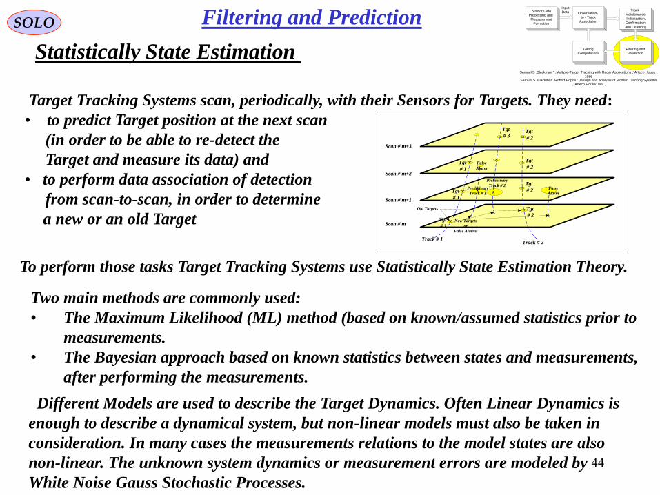
Statistically State Estimation
Target Tracking Systems scan, periodically, with their Sensors for Targets. They need:
• to predict Target position at the next scan
(in order to be able to re-detect the
Target and measure its data) and
• to perform data association of detection
from scan-to-scan, in order to determine
a new or an old TargetTrack # 1
Track # 2
New Targets
or
False Alarms
Old Targets
Scan # m
Scan # m+1
Scan # m+2
Scan # m+3
Tgt
# 1
Tgt
# 2
Tgt
# 1
Tgt
# 1
Tgt
# 2
Tgt
# 2
Tgt
# 2
Preliminary
Track # 1
Preliminary
Track # 2False
Alarm
False
Alarm
Tgt
# 3
To perform those tasks Target Tracking Systems use Statistically State Estimation Theory.
Two main methods are commonly used:
• The Maximum Likelihood (ML) method (based on known/assumed statistics prior to
measurements.
• The Bayesian approach based on known statistics between states and measurements,
after performing the measurements.
Different Models are used to describe the Target Dynamics. Often Linear Dynamics is
enough to describe a dynamical system, but non-linear models must also be taken in
consideration. In many cases the measurements relations to the model states are also
non-linear. The unknown system dynamics or measurement errors are modeled by
White Noise Gauss Stochastic Processes.
Filtering and PredictionSensor Data
Processing and
Measurement
Formation
Observation -
to - Track
Association
Input
DataTrack
Maintenance
(Initialization,
Confirmation
and Deletion)
Filtering and
Prediction
Gating
Computations
Samuel S . Blackman , " Multiple-Target Tracking with Radar Applications ", Artech House ,
1986Samuel S . Blackman , Robert Popoli , " Design and Analysis of Modern Tracking Systems
", Artech House , 1999

45
SOLO
Target Models as Markov Processes
Markov Random Processes
A Markov Random Process is defined by:
Andrei Andreevich
Markov
1856 - 1922
111
,|,,,|, tttxtxptxtxp
i.e. the Random Process, the past up to any time t1 is fully defined
by the process at t1.
Discrete Target Dynamic System
kkkkk
kkkkk
vuxthz
wuxtfx
,,,
,,, 1111
x - state space vector (n x 1)
u - input vector (m x 1)
- measurement vector (p x 1)z
v - white measurement noise vector (p x 1)
- white input noise vector (n x 1)w
kkkk
kkkk
vuxkhz
wuxkfx
,,,
,,,1 111
1ku
1k1kw
1kv
kz
Assumptions:
Known:
- functional forms f (•), h (•)
- noise statistics p (wk), p (vk)
- initial state probability density
function (PDF) p (x0)
Filtering and Prediction

46
SOLO
Discrete Target Dynamic System as Markov Processes
kkkkk
kkkkk
vuxthz
wuxtfx
,,,
,,, 1111
x - state space vector (n x 1)
u - input vector (m x 1)
- measurement vector (p x 1)z
v - white measurement noise vector (p x 1)
- white input noise vector (n x 1)w
Assumptions:
Known:
- functional forms f (•), h (•)
- noise statistics p (wk), p (vk)
- initial state probability density
function (pdf) p (x0)
Return to Table of Content
Using the k discrete (k=1,2,…) noisy measurements Z1:k={z1,z2,…,zk} we want to
estimate the hidden state xk, by filtering out the noise.
k – enumeration of the measurement events
The Estimator/Filter uses some assumptions about the model and an Optimization
Criteria to obtain the estimate of xk based on measurements Z1:k={z1,z2,…,zk} .
kkkk ZxEx :1| |ˆ
kkkk
kkkk
vuxkhz
wuxkfx
,,,
,,,1 111
1ku
1k1kw
1kv
kz
Filtering and Prediction

47
SOLO
Equation of motion of a point mass object are described by:
AIV
RI
V
R
td
d
x
x
xx
xx
33
33
3333
3333 0
00
0
A
V
R
- Range vector
- Velocity vector
- Acceleration vector
A
V
R
I
I
A
V
R
td
d
xxx
xxx
xxx
333333
333333
333333
000
00
00
or:
Since the target acceleration vector is not measurable, we assume that it is
a random process defined by one of the following assumptions:
A
1. White Noise Acceleration Model (Nearly Constant Velocity – nCV) .
3. Piecewise (between samples) Constant White Noise Acceleration Model .
5. Singer Acceleration Model .
2. Wiener Process acceleration model (nearly Constant Acceleration – nCA) .
4. Piecewise (between samples) Constant Wiener Process Acceleration Model
(Constant Jerk – a derivative of acceleration)
6. Constant Speed Turning Model .
Target motion is modeled using the laws of physics.
V
R
Bx
A
Target Acceleration Models
ModelContinuouswuxtFx
ModelDiscretewuxtfx kkkkk
,,,
,,, 1111
Filtering and Prediction
48
SOLO
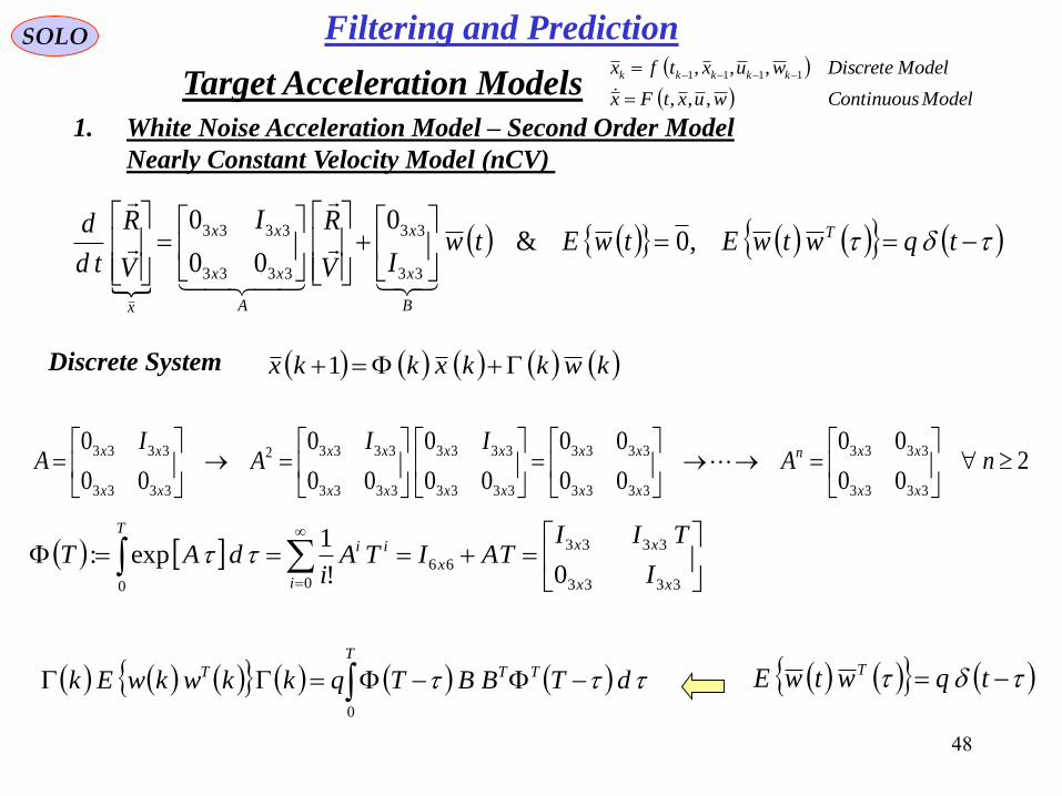
1. White Noise Acceleration Model – Second Order Model
Nearly Constant Velocity Model (nCV)
tqwtwEtwEtw
IV
RI
V
R
td
d T
B
x
x
A
xx
xx
x
,0&0
00
0
33
33
3333
3333
Discrete System kwkkxkkx 1
3333
3333
66
000!
1exp:
xx
xx
x
i
ii
T
I
TIITAITA
idAT
200
00
00
00
00
0
00
0
00
0
3333
3333
3333
3333
3333
3333
3333
33332
3333
3333
nA
IIA
IA
xx
xxn
xx
xx
xx
xx
xx
xx
xx
xx
tqwtwE T
T
TTT dTBBTqkkwkwEk0
Target Acceleration Models
ModelContinuouswuxtFx
ModelDiscretewuxtfx kkkkk
,,,
,,, 1111
Filtering and Prediction

49
SOLO
1. White Noise Acceleration Model (continue – 1)
Nearly Constant Velocity Model (nCV)
d
ITI
II
II
TIIq
xx
xx
xx
T
x
x
xx
xx
3333
3333
3333
0 33
33
3333
3333 00
0
0
T
TTTTT dTBBTqkkQkkkwkwEk0
d
ITI
TITIqdITI
I
TIq
T
xx
xxxx
T
x
x
0 3333
33
2
333333
0 33
33 2/
TITI
TITIqkkQk
xx
xxT
33
2
33
2
33
3
33
2/
2/3/
Guideline for Choice of Process Noise Intensity
The change in velocity over a sampling period T are of the order of TqQ 22
For a nearly constant velocity assumed by this model, the choice of q must be such
to give small changes in velocity compared to the actual velocity . V
Target Acceleration Models
ModelContinuouswuxtFx
ModelDiscretewuxtfx kkkkk
,,,
,,, 1111
Filtering and Prediction
50
SOLO
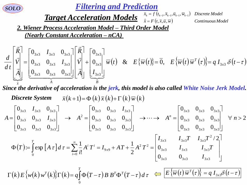
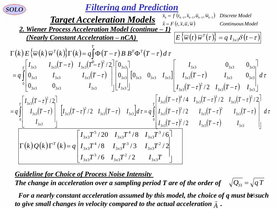
2. Wiener Process Acceleration Model – Third Order Model
(Nearly Constant Acceleration – nCA)
tIqwtwEtwEtw
IA
V
R
I
I
A
V
R
td
dx
T
B
x
x
x
A
xxx
xxx
xxx
x
33
33
33
33
333333
333333
333333
,0&0
0
000
00
00
Discrete System kwkkxkkx 1
333333
333333
2
333333
22
99
00 00
0
2/
2
1
!
1exp:
xxx
xxx
xxx
x
i
ii
T
I
TII
TITII
TATAITAi
dAT
2
000
000
000
000
000
00
000
00
00
333333
333333
333333
333333
333333
333333
2
333333
333333
333333
nA
I
AI
I
A
xxx
xxx
xxx
n
xxx
xxx
xxx
xxx
xxx
xxx
Since the derivative of acceleration is the jerk, this model is also called White Noise Jerk Model.
tIqwtwE x
T
33
T
TTT dTBBTqkkwkwEk0
Target Acceleration Models
ModelContinuouswuxtFx
ModelDiscretewuxtfx kkkkk
,,,
,,, 1111
Filtering and Prediction
51
SOLO
2. Wiener Process Acceleration Model (continue – 1)
(Nearly Constant Acceleration – nCA)
d
ITITI
ITI
I
I
II
TII
TITII
q
xxx
xxx
xxx
xxx
T
x
x
x
xxx
xxx
xxx
3333
2
33
333333
333333
333333
0
33
33
33
333333
333333
2
333333
2/
0
00
000
0
00
0
2/
T
TTT dTBBTqkkwkwEk0
d
ITITI
TITITI
TITITI
qdITITI
I
TI
TI
q
T
xxx
xxx
xxx
xxx
T
x
x
x
0
3333
2
33
33
2
33
3
33
2
33
3
33
4
33
3333
2
33
0
33
33
2
33
2/
2/
2/2/4/
2/
2/
TITITI
TITITI
TITITI
qkkQk
xxx
xxx
xxx
T
33
2
33
3
33
2
33
3
33
4
33
3
33
4
33
5
33
2/6/
2/3/8/
6/8/20/
Guideline for Choice of Process Noise Intensity
The change in acceleration over a sampling period T are of the order of TqQ 33
For a nearly constant acceleration assumed by this model, the choice of q must be such
to give small changes in velocity compared to the actual acceleration . A
tIqwtwE x
T
33
Target Acceleration Models
ModelContinuouswuxtFx
ModelDiscretewuxtfx kkkkk
,,,
,,, 1111
Filtering and Prediction

52
SOLO
3. Piecewise (between samples) Constant White Noise Acceleration Model – 2nd Order
,0&0
00
0
33
33
3333
3333
twEtw
IV
RI
V
R
td
d
B
x
x
A
xx
xx
x
Discrete System
kl
TTT lqkllwkwEkkwkkxkkx 01
3333
3333
66
000!
1exp:
xx
xx
x
i
ii
T
I
TIITAITA
idAT
200
00
00
00
00
0
00
0
00
0
3333
3333
3333
3333
3333
3333
3333
33332
3333
3333
nA
IIA
IA
xx
xxn
xx
xx
xx
xx
xx
xx
xx
xx
kw
TI
TIkw
Id
I
TIIdkTwBTkwk
x
x
x
xT
xx
xxT
kw
33
2
33
33
33
0 3333
3333
0
2/0
0:
Target Acceleration Models
ModelContinuouswuxtFx
ModelDiscretewuxtfx kkkkk
,,,
,,, 1111
Filtering and Prediction

53
SOLO
3. Piecewise (between samples) Constant White Noise Acceleration Model
klxx
x
x
kl
TTT TITITI
TIqlqkllwkwEk 33
2
33
33
2
33
00 2/2/
lk
xx
xxTT
TITI
TITIqllwkwEk ,2
33
3
33
3
33
4
33
02/
2/2/
Guideline for Choice of Process Noise Intensity
For this model q should be of the order of maximum acceleration magnitude aM.
A practical range is 0.5 aM ≤ q ≤ aM.
Target Acceleration Models
ModelContinuouswuxtFx
ModelDiscretewuxtfx kkkkk
,,,
,,, 1111
Filtering and Prediction

54
SOLO
4. Piecewise (between samples) Constant Wiener Process Acceleration Model
(Constant Jerk – a derivative of acceleration)
0&0
0
000
00
00
33
33
33
333333
333333
333333
twEtw
IA
V
R
I
I
A
V
R
td
d
B
x
x
x
A
xxx
xxx
xxx
x
Discrete System
lk
TTT lqkllwkwEkkwkkxkkx ,01
333333
333333
2
333333
22
99
00 00
0
2/
2
1
!
1exp:
xxx
xxx
xxx
x
i
ii
T
I
TII
TITII
TATAITAi
dAT
2
000
000
000
000
000
00
000
00
00
333333
333333
333333
333333
333333
333333
2
333333
333333
333333
nA
I
AI
I
A
xxx
xxx
xxx
n
xxx
xxx
xxx
xxx
xxx
xxx
kw
I
TI
TI
kwd
I
TII
TITII
dkTwBTkwk
x
x
xT
x
x
x
xxx
xxx
xxxT
kw
33
33
2
33
0
33
33
33
333333
333333
2
333333
0
2/
0
0
0
00
0
2/
:
Target Acceleration Models
ModelContinuouswuxtFx
ModelDiscretewuxtfx kkkkk
,,,
,,, 1111
Filtering and Prediction

55
SOLO
4. Piecewise (between samples) Constant White Noise acceleration model (continue -1)
(Constant Jerk – a derivative of acceleration)
lkxxx
x
x
x
lk
TTT ITITI
I
TI
TI
qlqkllwkwEk ,3333
2
33
33
33
2
33
0,0 2/
2/
lk
xxx
xxx
xxx
TT
ITITI
TITITI
TITITI
qllwkwEk ,
3333
2
33
33
2
33
3
33
2
33
3
33
4
33
0
2/
2/
2/2/2/
Guideline for Choice of Process Noise Intensity
For this model q should be of the order of maximum acceleration increment over a
sampling period ΔaM.
A practical range is 0.5 ΔaM ≤ q ≤ ΔaM.
Target Acceleration Models
ModelContinuouswuxtFx
ModelDiscretewuxtfx kkkkk
,,,
,,, 1111
Filtering and Prediction

56
SOLO
5. Singer Target Model
R.A. Singer, “Estimating Optimal Tracking Filter Performance for Manned Maneuvering
Target”, IEEE Trans. Aerospace & Electronic Systems”, Vol. AES-6, July 1970,
pp. 437-483
The target acceleration is modeled as a zero-mean random process with exponential
autocorrelation TetataER mTT
/2
where σm2 is the variance of the target acceleration and τT is the time constant of its
autocorrelation (“decorrelation time”).
The target acceleration is assumed to:
1. Equal to the maximum acceleration value amax
with probability pM and to – amax
with the same probability.
2. Equal to zero with probability p0.
3. Uniformly distributed between [-amax, amax]
with the remaining probability 1-2 pM – p0 > 0.maxa
maxa
Mp Mp
0p
ap
a
021 ppM
max
0maxmax0maxmax
2
210
a
ppaauaauppaaaaap M
M
Target Acceleration Models
ModelContinuouswuxtFx
ModelDiscretewuxtfx kkkkk
,,,
,,, 1111
Filtering and Prediction

57
SOLO
5. Singer Target Model (continue 1)
maxamaxa
Mp Mp
0p
ap
a
021 ppM
max
0maxmax0maxmax
2
210
a
ppaauaauppaaaaap M
M
022
210
2
21
0
max
max
max
max
max
max
max
max
2
max
00maxmax
max
0maxmax
0maxmax
a
a
MM
a
a
M
a
a
M
a
a
a
a
ppppaa
daaa
ppaauaau
daappaaaadaapaaE
0
2
max
3
max
02
max
2
max
2
max
0maxmax
2
0maxmax
22
413
32
21
2
21
0
max
max
max
max
max
max
max
max
ppa
a
a
pppaa
daaa
ppaauaau
daappaaaadaapaaE
M
a
a
MM
a
a
M
a
a
M
a
a
0
2
max
0
22241
3pp
aaEaE Mm
Use
max0max
00
max
max
aaa
afdaafaa
a
a
Target Acceleration Models
ModelContinuouswuxtFx
ModelDiscretewuxtfx kkkkk
,,,
,,, 1111
Filtering and Prediction

58
SOLO
6. Target Acceleration Approximation by a Markov Process
w (t) x (t)
tF
tG
x (t)
twtGtxtFtxtxtd
d Given a Continuous Linear System:
Let start with the first order linear system describing Target Acceleration :
twtata T
T
T
1
T
T
tt
a ett /
00,
tqwEwtwEtwE
ttRtaEtataEtaETT aaTTTT ,
ttRtaEtataEtaETT aaTTTT ,
2,
TTTTT aaaaaTTTT ttRtVtaEtataEtaE
tGtQtGtFtVtVtFtVtd
d TT
xxx qtVtV
td
dTTTT aa
T
aa
2
00 ,1
, tttttd
dTT a
T
a
where
Target Acceleration Models
ModelContinuouswuxtFx
ModelDiscretewuxtfx kkkkk
,,,
,,, 1111
Filtering and Prediction
Run This

59
SOLO
qtVtVtd
dTTTT aa
T
aa
2
TT
TTTT
t
T
t
aaaa eq
eVtV 22
12
0t
2/T
T
t
wweV
2
0
T
t
eqT
2
12
2
qTV statesteadyww
tVww
0,
0,,
tVetttV
tVetVttttR
TT
T
TTT
TT
T
TTT
TT
aa
T
aaa
aaaaa
aa
0,
0,,
tVetVtt
tVetttVttR
TT
T
TTT
TT
T
TTT
TT
aaaaa
aa
T
aaa
aa
For 2
5 Tstatesteadyaaaaaa
T
qVtVtV
TTTTTT
TT
TTTTTTTTe
qeVVttRttR
T
Tstatesteadyaaaaaaaa
2
,,5
tw taT T
T
ssH
1
6. Target Acceleration Approximation by a Markov Process (continue – 1)
Target Acceleration Models
ModelContinuouswuxtFx
ModelDiscretewuxtfx kkkkk
,,,
,,, 1111
Run This

60
SOLO
T
T
T
TTee
qV a
Taa
/2/
2
2
2 Ta
qT
T
12 eTa
T
2
02
2 TT
aa qdeq
dVArea T
TT
τT is the correlation time of the noise w (t) and defines in Vaa (τ) the correlation
time corresponding to σa2 /e.
One other way to find τT is by tacking the double sides Laplace Transform L2 on τ of:
qdetqtqs s
ww
2L
sHqsH
s
q
deeq
Vs
T
T
sTssaaaa
T
TTTT
2
2
/
2
1
2
L
22/1/1
q
Qww
T /12/1
q
2/q
T /12/1
τT defines the ω1/2 of half of the power spectrum
q/2 and τT =1/ ω1/2.
TT
TTTTTTTe
qeVttRttR
T
Taaaaaaa
2
,,52
T
aTq
2
2
6. Target Acceleration Approximation by a Markov Process (continue – 2)
Target Acceleration Models
ModelContinuouswuxtFx
ModelDiscretewuxtfx kkkkk
,,,
,,, 1111
Filtering and Prediction
Run This
61
SOLO
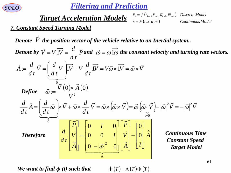
7. Constant Speed Turning Model
Denote by and the constant velocity and turning rate vectors.Ptd
dVVV
1 1
VVVVtd
dVVV
td
dV
td
dA
111:
0
VVVVVtd
dV
td
dA
td
d
22
0:
0
Define
2
00:
V
AV
Denote the position vector of the vehicle relative to an Inertial system..P
We want to find ф (t) such that TTT
Therefore A
IA
V
P
I
I
A
V
P
td
d
0
0
00
00
00
2
Continuous Time
Constant Speed
Target Model
Target Acceleration Models
ModelContinuouswuxtFx
ModelDiscretewuxtfx kkkkk
,,,
,,, 1111
Filtering and Prediction

62
SOLO
7. Constant Speed Turning Model (continuous – 1)
A
BC
O
n
v
1v
Let rotate the vector around by a large angle
, to obtain the new vector
OAPT
n
T
OBP
From the drawing we have:
CBACOAOBP
TPOA
cos1ˆˆ
TPnnAC Since direction of is: sinˆˆ&ˆˆ
TTT PPnnPnn
and it’s length is:
AC
cos1sin TP
sinˆTPnCB
Since has the direction and the
absolute value
CB
TPn
ˆsinsinv
sinˆcos1ˆˆTTT PnPnnPP
TPnTPnnPP TTT sinˆcos1ˆˆ
We will find ф (T) by direct computation of a rotation:
Target Acceleration Models
ModelContinuouswuxtFx
ModelDiscretewuxtfx kkkkk
,,,
,,, 1111
Filtering and Prediction
Run This
63
SOLO
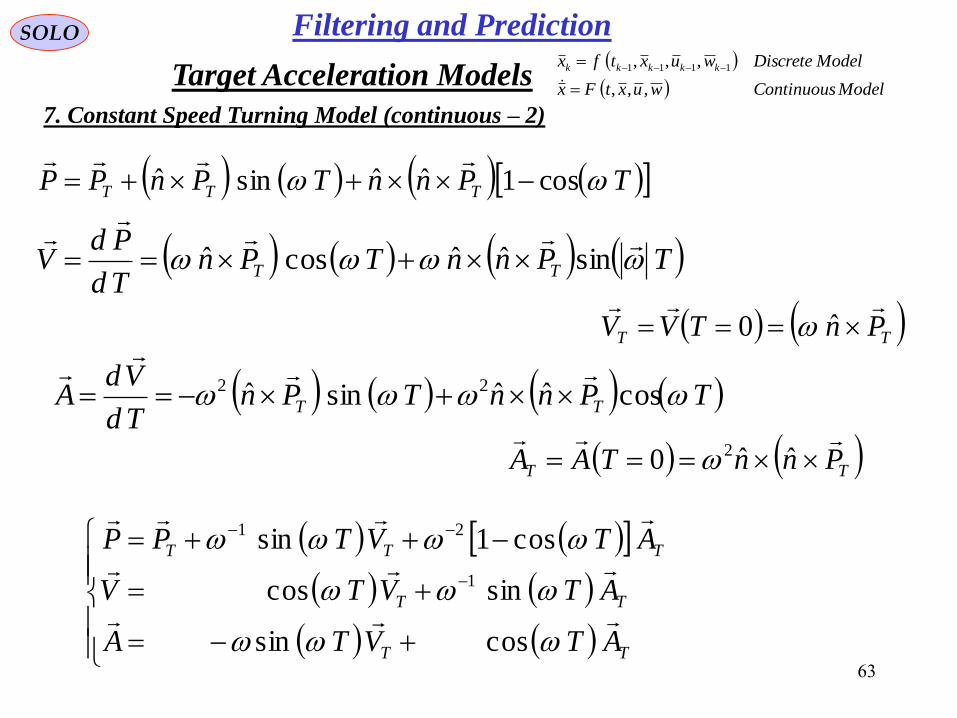
7. Constant Speed Turning Model (continuous – 2)
TPnnTPnTd
PdV TT
sinˆˆcosˆ
TT PnTVV
ˆ0
TPnnTPnTd
VdA TT cosˆˆsinˆ 22
TT PnnTAA
ˆˆ0 2
TT
TT
TTT
ATVTA
ATVTV
ATVTPP
cossin
sincos
cos1sin
1
21
TPnnTPnPP TTT cos1ˆˆsinˆ
Target Acceleration Models
ModelContinuouswuxtFx
ModelDiscretewuxtfx kkkkk
,,,
,,, 1111
Filtering and Prediction

64
SOLO
7. Constant Speed Tourning Model (continuous – 3)
TT
TT
TTT
ATVTA
ATVTV
ATVTPP
cossin
sincos
cos1sin
1
21
T
T
T
T
A
V
P
TT
TT
TTI
A
V
P
cossin0
sincos0
cos1sin
1
21
Discrete Time
Constant Speed
Target Model
Target Acceleration Models
ModelContinuouswuxtFx
ModelDiscretewuxtfx kkkkk
,,,
,,, 1111
Filtering and Prediction

65
SOLO
7. Constant Speed Tourning Model (continuous – 4)
TT
TT
TTI
T
cossin0
sincos0
cos1sin
1
21
TT
TT
TTI
T
cossin0
sincos0
cos1sin
1
21
1
TT
TT
TT
T
sincos0
cossin0
sincos0
2
1
We want to find Λ (t) such that
TTT therefore TTT 1
TT
TT
TTI
TT
TT
TT
TTT
cossin0
sincos0
cos1sin
sincos0
cossin0
sincos01
21
2
1
1
00
100
010
2
We recovered the transfer matrix for the continuous
case.
Return to Table of Content
Target Acceleration Models
ModelContinuouswuxtFx
ModelDisccretewuxtfx kkkkk
,,,
,,, 1111
Filtering and Prediction
66
SOLO
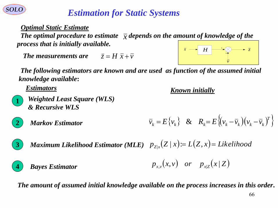
Optimal Static Estimate
The optimal procedure to estimate depends on the amount of knowledge of the
process that is initially available.x
The following estimators are known and are used as function of the assumed initial
knowledge available:
Estimators Known initially
Weighted Least Square (WLS)
& Recursive WLS1
T
kkkkkkk vvvvERvEv &Markov Estimator2
Maximum Likelihood Estimator (MLE)3 LikelihoodxZLxZp xZ ,:||
Bayes Estimator4 Zxporvxp Zxvx |, |,
The amount of assumed initial knowledge available on the process increases in this order.
Estimation for Static Systems
v
H zx
The measurements are vxHz

67
Estimation for Static Systems (continue – 1)SOLO
Parameter Vector: full specification of (static) parameters to be estimated
Measurements:
• collected over time and/or space
• affected by noise
vRx
,Examples: or avRx
,,
a
v
R
Position 3 D vector
Velocity 3 D vector
Acceleration 3 D vector
• relationship (nonlinear/linear) with parameter vector
m
k
n
kk RzRxKkvxhz ,;,,1
Goal: Estimate the Parameter Vector using all measurementx
Approaches:
• treat as being deterministic (Minimal Least Square -MLE, LSE) x
• treat as being random (MAP Estimator, MMSE Estimator) x

68
z
SOLO
Optimal Weighted Last-Square Estimate
Assume that the set of p measurements, can be expressed as a linear combination,
of the elements of a constant vector plus a random, additive measurement error, :
v
H zx
x v
vxHz
1
1
W
TxHzxHzWxHzJ
Tp
zzzz ,,,21
Tn
xxxx ,,,21
Tp
vvvv ,,,21
We want to find , the estimation of the constant vector , that minimizes the
cost function:
x
x
that minimizes J, is obtained by solving:0x
02/ 1 xHzWHxJJ T
x
zWHHWHx TT 111
0
This solution minimizes J iff :
02/0
1
00
22
0 xxHWHxxxxxJxx TTT
or the matrix HTW-1H is positive definite.
W is a hermitian (WH = W, H stands for complex conjugate and matrix transpose),
positive definite weighting matrix.
Estimation for Static Systems (continue – 2)

69
v
H zx
SOLO
Optimal Weighted Least-Square Estimate (continue – 1)
zWHHWHx TT 111
0
Since the mean of the estimate is equal to the estimated parameter, the estimator
is unbiased.
vxHz Since is random with mean
xHvExHvxHEzE 0
xxHWHHWHzEWHHWHxE TTTT 111111
0
is also random with mean:0
x
0
1
00
12
00
1
0
* : xHzWHxxHzWzxHzxHzWxHzJ TTT
W
T
Using we want to find the minimum value of J:0
11 xHWHzWH TT
0
1
0
0
11
00
1 xHzWzxHWHzWHxxHzWz TTTTT
2
0
2
0
1
0
1
0
11
1
0
WW
TTT
HWHx
TT xHzxHWHxzWzxHWzzWzTT
Estimation for Static Systems (continue – 3)
70
v
H zx
2
0
22
0
*111
WWWxHzxHzJ
SOLO
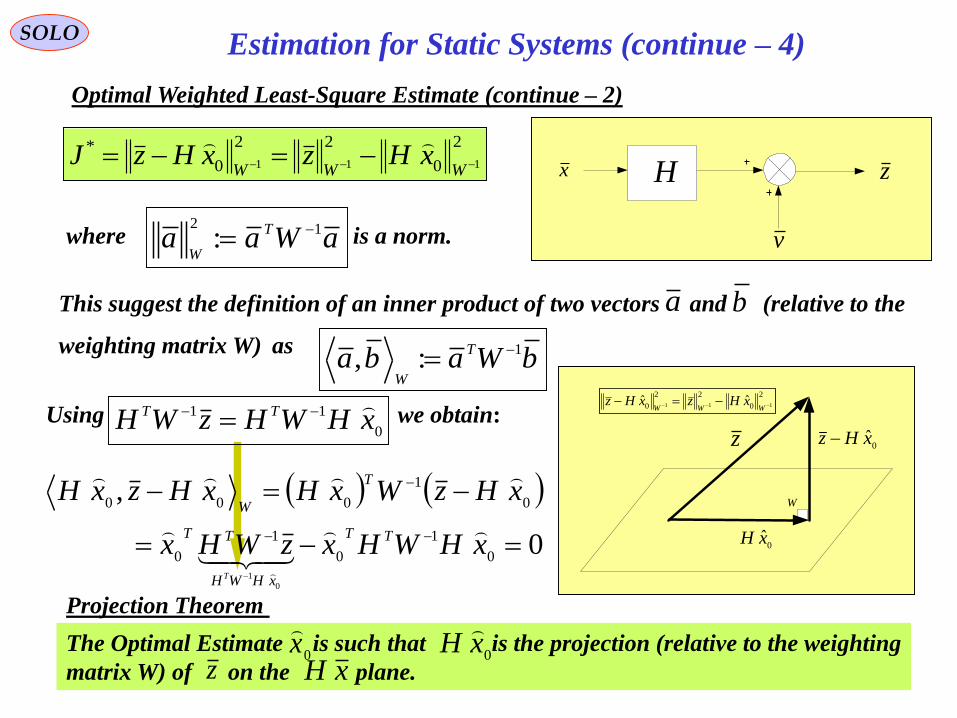
Optimal Weighted Least-Square Estimate (continue – 2)
where is a norm.aWaa T
W
12
:
Using we obtain:0
11 xHWHzWH TT
0
,
0
1
0
1
0
0
1
000
0
1
xHWHxzWHx
xHzWxHxHzxH
TT
xHWH
TT
T
W
T
bWaba T
W
1:,
This suggest the definition of an inner product of two vectors and (relative to the
weighting matrix W) as
ba
z 0xHz
0xH
W
2
0
22
0 111 ˆˆ WWW
xHzxHz
Projection Theorem
The Optimal Estimate is such that is the projection (relative to the weighting
matrix W) of on the plane.0
x
z0
xH
xH
Estimation for Static Systems (continue – 4)

72
0z
SOLO
Recursive Weighted Least Square Estimate (RWLS)
Assume that the set of N measurements, can be expressed as a linear combination,
of the elements of a constant vector plus a random, additive measurement error, :
0v
0zx
0H
x vvxHz
00
10
0000
1
0000
W
TxHzxHzWxHzJ
We found that the optimal estimator ,
that minimizes the cost function:
x
0
1
00
1
0
1
00zWHHWHx
TT
is
Let define the following matrices for the complete measurement set
W
WW
z
zz
H
HH
0
0:,:,:
0
1
0
1
0
1 1
0
1
00:
HWHP
T
Therefore:
1
1 1
0 0 0 01 1
1 1 1 1 1 1 0 01 1
0 0
0 0
T T T T T TW H W z
x H W H H W z H H H HH zW W
v
H zx
0
1
00zWHPx
T
An additional measurement set, is obtained
and we want to find the optimal estimator . z
x
Estimation for Static Systems (continue – 5)

73
SOLO
Recursive Weighted Least Square Estimate (RWLS) (continue -1)
1
0
1
00:
HWHP
T 0
1
00zWHPx
T
zWHzWHHWHHWH
z
z
W
WHH
H
H
W
WHHzWHHWHx
TTTT
TTTTTT
1
0
1
00
11
0
1
00
0
1
1
0
0
1
0
1
1
0
01
1
111
1
11
0
0
0
0
Define HWHPHWHHWHP TTT 111
0
1
00
1 :
PHWHPHHPPHWHPP TT
LemmaMatrixInverseT 1111
111111
WHPWHHWHPWHPHHP TTTTT
PHWHPPPHWHPHHPPP TTT 11
zWHPzWHPHWHPHHPP
zWHzWHPx
TTTT
TT
1
0
1
00
1
1
0
1
00
Estimation for Static Systems (continue – 6)

74
v
H zx
SOLO
Recursive Weighted Least Square Estimate (RWLS) (continue -2)
zWHPxHWHPx
zWHPzWHPHWHPHHPzWHP
zWHPzWHPHWHPHHPP
zWHzWHPx
TT
T
x
T
WHP
TT
x
T
TTTT
TT
T
11
1
0
1
00
1
0
1
00
1
0
1
00
1
1
0
1
00
1
0
1
00zWHPx
T
HWHPP T 111
xHzWHPxx T 1
Recursive Weighted Least Square Estimate
(RWLS)
z
x
x
Delay
HWHP T 11
H
1 WHP T
Estimator
Estimation for Static Systems (continue – 7)
75
xHzWxHzxHzWxHz
xHz
xHz
W
WxHzxHz
xHz
xHz
W
W
xHz
xHzxHzWxHzJ
TT
TT
T
T
1
00
1
000
00
1
1
0
00
00
1
000
11
1
1111
0
0
0
0
0
1
00
1 : HWHPT
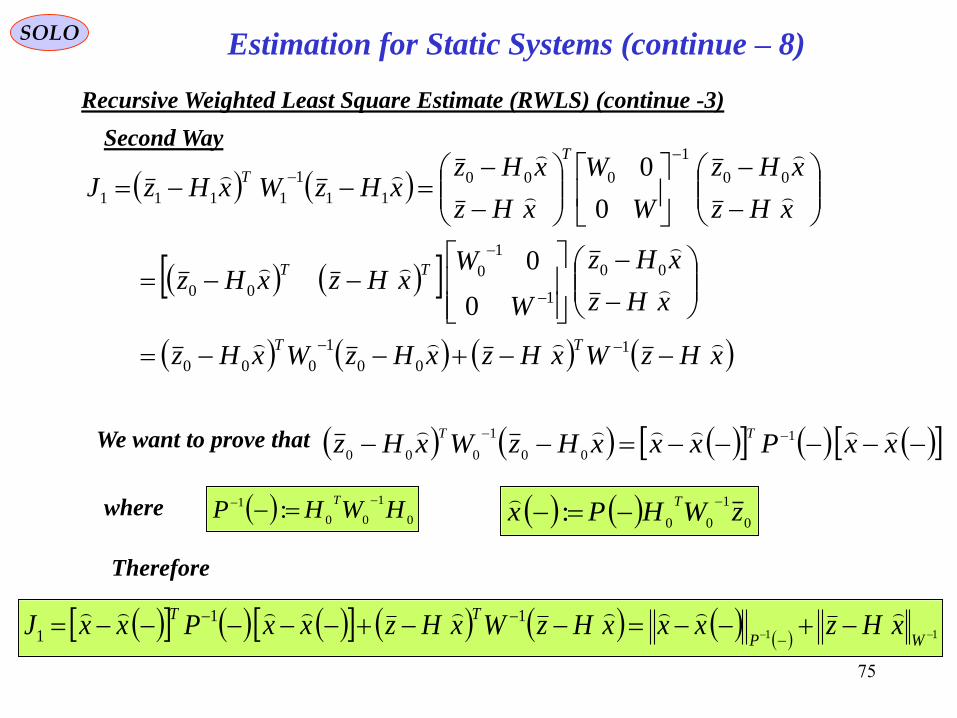
SOLO
Recursive Weighted Least Square Estimate (RWLS) (continue -3)
Second Way
We want to prove that
where 0
1
00: zWHPx
T
xxPxxxHzWxHz
TT 1
00
1
000
Therefore
11
11
1
WP
TTxHzxxxHzWxHzxxPxxJ
Estimation for Static Systems (continue – 8)

76
Estimators
vxHz 00
v
0H0zx
SOLO
Markov Estimate
For the particular vector measurement equation
where for the measurement noise, we know the mean: vEv
and the variance: TvvvvER
v
zRHHRHxTT 1
0
1
0
1
00
We choose W = R in WLS, and we obtain:
1
0
1
0:
HRHPT
HRHPP T 111
xHzRHPxx T 1
RWLS = Markov Estimate
W = R
z
x
x
Delay
HRHP T 11
H
1 RHP T
Estimator
In Recursive WLS, we obtain for a new
observation: vxHz v
H zx
Table of Content

77
Estimation for Static Systems (continuous – 9)SOLO
k
k
k
kk
Zp
xpxZp
dxxpxZp
xpxZpZxp
|
|
||
Bayesian Approach: compute the posteriori Probability Density Function (PDF) of x
kk zzZ ,,1 - Measurements up to k
xp - Prior (before measurement) PDF of x
xZLxZp kk ,| - Likelihood function of given xkZ
kZxp | - Posterior (after measurement ) PDF of xkZ
Likelihood Function: PDF of measurement conditioned on the parameter vector
Example kk vxhz
2,0;~ vk vv N i.i.d. process; k=1,…,K
(independent identical distribution)
2
| ,;~| vkxz xhzxzpk
N
K
k
kxzkxZ xzpxZpkk
1
|| ||
Bayes Formula

78
Estimation for Static Systems (continuous – 10)SOLO
k
T
xk
MMSE ZxxxxEZx |ˆˆminargˆˆ
Minimum Mean Square Error (MMSE) Estimator
The minimum is given by
0|ˆ2|ˆ2|ˆˆˆ kkk
T
x ZxExZxxEZxxxxE
From which
xdZxpxZxEx kZxk k|| |
*
We have 02|ˆˆˆˆ k
T
xx ZxxxxE
xdZxpxZxEZxxxxEZx kZxkk
T
xk
MMSE
k|||ˆˆminargˆ
|ˆ
Therefore
79
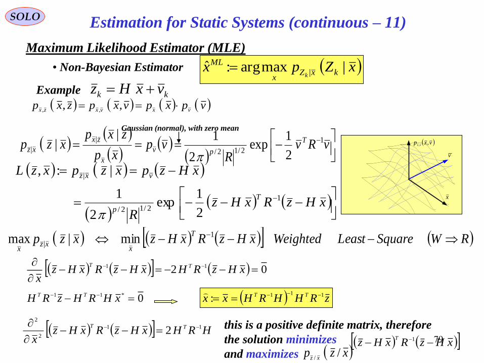
Estimation for Static Systems (continuous – 11)SOLO
Maximum Likelihood Estimator (MLE)
xZpx kxZx
ML
k|maxarg:ˆ
|• Non-Bayesian Estimator
vpxpvxpzxpvxvxzx
,,,,
x
v
vxpvx
,,
xHzRxHzR
xHzpxzpxzL
T
p
vxz
1
2/12/
|
2
1exp
2
1
|:,
RWSquareLeastWeightedxHzRxHzxzpT
xxz
x 1
| min|max
02 11
xHzRHxHzRxHzx
TT
0*11 xHRHzRH TT zRHHRHxx TT 111:
HRHxHzRxHzx
TT 11
2
2
2
this is a positive definite matrix, therefore
the solution minimizes
and maximizes xHzRxHz
T 1
xzpxz
//
vRv
Rvp
xp
zxpxzp T
pv
x
zx
xz
1
2/12/
|
|2
1exp
2
1||
Gaussian (normal), with zero mean
Example kk vxHz

80
Estimation for Static Systems (continuous – 12)SOLO
Maximum A Posterior Estimator (MAP)
xpxZpZxpx xkxZx
kZxx
MAP
kk|maxarg|maxarg:ˆ
|| •Bayesian Estimator
xxPxx
Pxp
T
nx
1
2/12/ 2
1exp
2
1
xHzRxHz
RxHzpxzp
T
pvxz
1
2/12//2
1exp
2
1/
xHzRHPHxHzRHPH
zp TT
Tpz
1
2/12/ 2
1exp
2
1
xHzRHPHxHzxxPxxxHzRxHz
RHPH
RPzp
xpxzpzxp
TTTT
T
nz
xxz
zx
111
2/1
2/12/1
2/
|
|
2
1
2
1
2
1exp
2
1||
from which
vxHz Consider a gaussian vector , where , measurement, ,
where the gaussian noise is independent of and . RNv ,0~v
x PxNx ,~
x

81
SOLO
xHzRHPHxHzxxPxxxHzRxHz TTTT
111
11111111 RHPHRHHRRRRHPHR TTTwe have
then
Define: 111: HRHPP T
xHzRHxxPxHzRHxx TTT 111
xHzRHPxxPxHzRHPxxP
zxp TTT
nzx
111
2/12/|2
1exp
2
1|
then
zxp zxx
|max | xHzRHPxxx T 1*:
Estimation for Static Systems (continuous – 13)
Maximum A Posterior Estimator (MAP) (continue – 1)
xpxZpZxpx xkxZx
kZxx
MAP
kk|maxarg|maxarg:ˆ
|| •Bayesian Estimator
For Diffuse Uniform a Priori constxpx
MLE
kxZx
kZxx
MAP xxZpZxpxkk
ˆ|maxarg|maxarg:ˆ||

82
SOLO
Optimal Static Estimate (Summary)
EstimatorsKnown initially
Weighted Least Square (WLS)1
T
kkkkkkk vvvvERvEv &
Markov Estimator2
Estimation for Static Systems
2
0
22
0
*111
WWWxHzxHzJ
v
H zx
z 0xHz
0xH
W
2
0
22
0 111 ˆˆ WWW
xHzxHz
The measurements are
vxHz
1
1
W
TxHzxHzWxHzJ zWHHWHx TTWLS 111
& Recursive WLS
Jxmin
HWHPHWHHWHP TTT 111
0
1
00
1
xHzWHPxx T 1Recursive Weighted Least Square Estimate
(RWLS)
z
x
x
Delay
HWHP T 11
H
1 WHP T
Estimator
HRHPHRHHRHP TTT 111
0
1
0
1
xHzRHPxx T 1RWLS = Markov Estimator
W = R
z
x
x
Delay
HRHP T 11
H
1 RHP T
Estimator
No assumption about noise v
Assumption about noise v

83
SOLO
Optimal Static Estimate (Summary)
Estimators Known initially
Maximum Likelihood Estimator (MLE)3 LikelihoodxZLxZp xZ ,:||
Bayes Estimator – Maximum Apriory
Estimator (MAP)
4 Zxporvxp Zxvx |, |,
Estimation for Static Systems
xHzRxHz
RxHzpxzpxzL
T
pvxz
1
2/12/|2
1exp
2
1|:,
v
H zx
RWSquareLeastWeightedxHzRxHzxzpT
xxz
x 1
| min|max
The measurements are
vxHz
zRHHRHx TTML 111
xpZxpZxpx XxZX
ZxX
MAP |maxarg|maxargˆ||
84
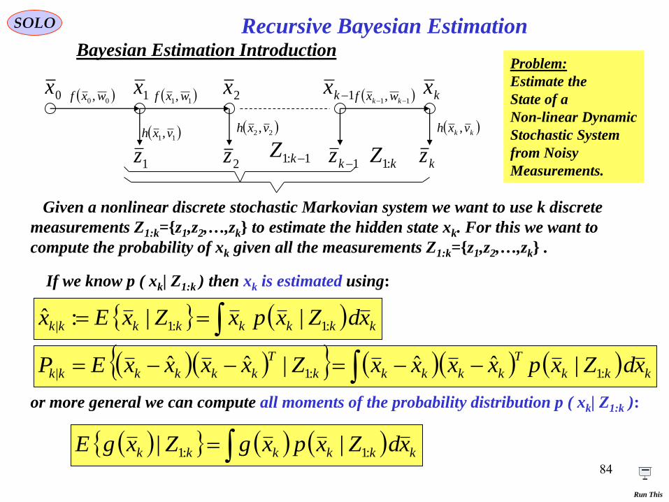
Recursive Bayesian EstimationSOLO
Given a nonlinear discrete stochastic Markovian system we want to use k discrete
measurements Z1:k={z1,z2,…,zk} to estimate the hidden state xk. For this we want to
compute the probability of xk given all the measurements Z1:k={z1,z2,…,zk} .
If we know p ( xk| Z1:k ) then xk is estimated using:
kkkkkkkk xdZxpxZxEx :1:1| ||:ˆ
kkk
T
kkkkk
T
kkkkkk xdZxpxxxxZxxxxEP :1:1| |ˆˆ|ˆˆ
or more general we can compute all moments of the probability distribution p ( xk| Z1:k ):
kkkkkk xdZxpxgZxgE :1:1 ||
Bayesian Estimation IntroductionProblem:
Estimate the
State of a
Non-linear Dynamic
Stochastic System
from Noisy
Measurements.
kx1kx
kz1kz
0x 1x 2x
1z 2z kZ :11:1 kZ
11, kk wxf
kk vxh ,
00 , wxf
11,vxh
11, wxf
22 ,vxh
Run This
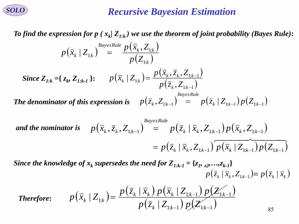
85
Recursive Bayesian EstimationSOLO
To find the expression for p ( xk| Z1:k ) we use the theorem of joint probability (Bayes Rule):
k
kkRuleBayes
kkZp
ZxpZxp
:1
:1:1
,|
Since Z1:k ={ zk, Z1:k-1 }: 1:1
1:1:1
,
,,|
kk
kkkkk
Zzp
ZzxpZxp
The denominator of this expression is
1:11:11:1 ,,|,, kkkkk
RuleBayes
kkk ZxpZxzpZzxp
1:11:11:1 |,| kkkkkk ZpZxpZxzp
Since the knowledge of xk supersedes the need for Z1:k-1 = {z1, z2,…,zk-1}
kkkkk xzpZxzp |,| 1:1
1:11:1
1:11:1:1
|
|||
kkk
kkkkkkk
ZpZzp
ZpZxpxzpZxpTherefore:
1:11:11:1 |, kkk
RuleBayes
kk ZpZzpZzp
and the nominator is

86
Recursive Bayesian EstimationSOLO
The final result is:
1:1
1:1:1
|
|||
kk
kkkkkk
Zzp
ZxpxzpZxp
1:1
1:1
1:1
1:1:1
|
||
|
|||1
kk
kkkkk
k
kk
kkkkkkk
Zzp
xdZxpxzpxd
Zzp
ZxpxzpxdZxp
Since p ( xk| Z1:k ) is a probability distribution it must satisfy: 1| :1 kkk xdZxp
kkkkk
kkkkkk
xdZxpxzp
ZxpxzpZxp
1:1
1:1:1
||
|||
and:
Therefore: kkkkkkk xdZxpxzpZzp 1:11:1 |||
This is a recursive relation that needs the value of p (xk|Z1:k-1), assuming that
p (zk,xk) is obtained from the Markovian system definition.
kx1kx
kz1kz
0x 1x 2x
1z 2z kZ :11:1 kZ
11, kk wxf
kk vxh ,
00 , wxf
11,vxh
11, wxf
22 ,vxh

87
Recursive Bayesian EstimationSOLO
11:111:111:11 |,||, kkkkkk
Bayes
kkk xdZxpZxxpZxxpUsing:
11:11111:111:1 |||,| kkkkkkkkkkk xdZxpxxpxdZxxpZxp
We obtain:
Since the knowledge of xk-1 supersedes the need for Z1:k-1 = {z1, z2,…,zk-1}
11:11 |,| kkkkk xxpZxxp
kx1kx
kz1kz
0x 1x 2x
1z 2z kZ :11:1 kZ
11, kk wxf
kk vxh ,
00 , wxf
11,vxh
11, wxf
22 ,vxh
Chapman – Kolmogorov Equation
Sydney Chapman
1888 - 1970
Andrey
Nikolaevich
Kolmogorov
1903 - 1987

88
Recursive Bayesian EstimationSOLO
11:11111:111:1 |||,| kkkkkkkkkkk xdZxpxxpxdZxxpZxp
Summary
Using p (xk-1|Z1:k-1) from time-step k-1 and p (xk|xk-1) of the Markov system, compute:
kkkkk
kkkkkk
xdZxpxzp
ZxpxzpZxp
1:1
1:1:1
||
|||
Using p (xk|Z1:k-1) from Prediction phase and p (zk|xk) of the Markov system, compute:
kkkkkkkk xdZxpxZxEx :1:1| ||ˆ
kkk
T
kkkkk
T
kkkkkk xdZxpxxxxZxxxxEP :1:1| |ˆˆ|ˆˆ
At stage k
k:=k+1
1|11|ˆˆ
kkkk xfx
Initialize with p (x0)0
Prediction phase
(before zk measurement)
1
Correction Step (after zk measurement)2
Filtering3
kx1kx
kz1kz
0x 1x 2x
1z 2z kZ :11:1 kZ
11, kk wxf
kk vxh ,
00 , wxf
11,vxh
11, wxf
22 ,vxh

89
SOLO
Linear Gaussian Systems
A Linear Combination of Independent Gaussian random vectors is also a
Gaussian random vectormmm XaXaXaS 2211:
mmmm
mmmm
YYYm
YpYp
mYYmS
aaajaaa
ajaajaaja
YdYdYYpSjm
mmYY
mm
2211
222
2
2
2
2
1
2
1
2
222
22
2
2
2
2
2
11
2
1
2
1
2
11,,
2
1exp
2
1exp
2
1exp
2
1exp
,,exp21
11
1
2
2
2exp
2
1,;
i
ii
i
iiiX
XXp
i
Gaussian
distribution
iiiiXiX jXdXpXjii
22
2
1expexp:
Moment-
Generating
Function
Proof:
Define iX
ii
iX
i
iYiii Xpaa
Yp
aYpXaY
iii
11:
iiiiiiX
asign
asign
ii
i
iX
iiiiYiY ajaXaXdaa
XpXajYdYpYj
i
i
ii
222
2
1expexpexp:
1
1
Review of Probability

90
SOLO
Linear Gaussian Systems
A Linear Combination of Independent Gaussian random vectors is also a
Gaussian random vectormmm XaXaXaS 2211:
Therefore the Linear Combination of Independent Gaussian Random Variables is a
Gaussian Random Variable with
mmS
mmS
aaa
aaa
m
m
2211
222
2
2
2
2
1
2
1
2
Therefore the Sm probability distribution is:
2
2
2exp
2
1,;
m
m
m
mm
S
S
S
SSm
xSp
Proof (continue – 1):
mmmmS aaajaaa
m 2211
222
2
2
2
2
1
2
1
2
2
1exp
We found:
Review of Probability
q.e.d.
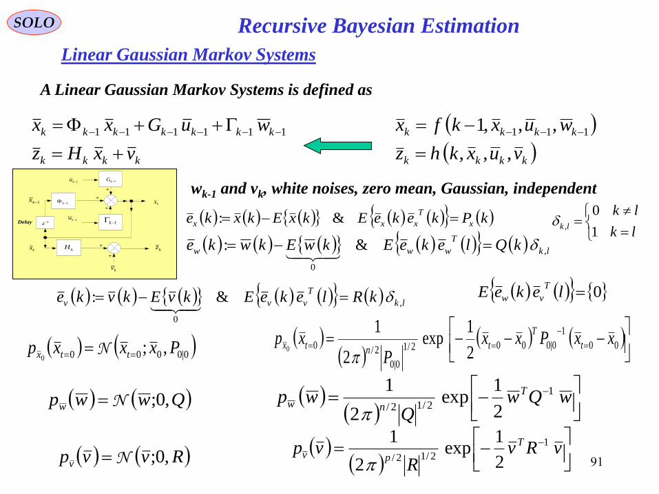
91
Recursive Bayesian EstimationSOLO
Linear Gaussian Markov Systems
kkkk
kkkk
vuxkhz
wuxkfx
,,,
,,,1 111
kkkk
kkkkkkk
vxHz
wuGxx
111111
wk-1 and vk, white noises, zero mean, Gaussian, independent
kPkekeEkxEkxke x
T
xxx &:
lk
T
www kQlekeEkwEkwke ,
0
&:
lk
T
vvv kRlekeEkvEkvke ,
0
&:
0lekeET
vw
lk
lklk
1
0,
kv
kH kzkx
kx1 k
1kw1k
1kx
1ku 1kG
1zDelay
Qwwpw ,0;N
Rvvpv ,0;N
wQw
Qwp T
nw
1
2/12/ 2
1exp
2
1
vRv
Rvp T
pv
1
2/12/ 2
1exp
2
1
A Linear Gaussian Markov Systems is defined as
0|0000 ,;0
Pxxxp ttx N
00
1
0|0002/1
0|0
2/02
1exp
2
10
xxPxxP
xp t
T
tntx

92
Recursive Bayesian EstimationSOLO
Linear Gaussian Markov Systems (continue – 1)
111111 kkkkkkk wuGxxkx1 k
1kw1k
1kx
1ku 1kGPrediction phase (before zk measurement)
or 111|111|ˆˆ
kkkkkkk uGxx
0
1:111111:1111:11| |||:ˆ kkkkkkkkkkkk ZwEuGZxEZxEx
The expectation is
1:1111|111111|111
1:11|1|1|
|ˆˆ
|ˆˆ:
k
T
kkkkkkkkkkkk
k
T
kkkkkkkk
ZwxxwxxE
ZxExxExEP
T
k
Q
T
kkk
T
k
T
kkkkk
T
k
T
kkkkk
T
k
P
T
kkkkkkk
wwExxwE
wxxExxxxE
kk
11111
0
1|1111
1
0
11|11111|111|111
ˆ
ˆˆˆ
1|1
T
kk
T
kkkkkk QPP 1111|111|
1|1|1:1 ,ˆ;| kkkkkkk PxxZxP N
Since is a Linear Combination of Independent
Gaussian Random Variables:111111 kkkkkkk wuGxx

93
Recursive Bayesian EstimationSOLO
Linear Gaussian Markov Systems (continue – 9)
kkkk vxHz kv
kH kzkx
Rvvpv ,0;N
vRv
Rvp T
pv
1
2/12/ 2
1exp
2
1
1|
1
1|1|2/1
1|
2/ˆˆ
2
1exp
2
1kkkkk
T
kkkk
T
kkkk
k
T
kkkk
pkz xHzRHPHxHz
RHPHzp
from which 1|1:11|ˆ|ˆ
kkkkkkk xHZzEz
kk
T
kkkkk
T
kkkkkk
zz
kk SRHPHZzzzzEP :ˆˆ1|1:11|1|1|
T
kkkk
T
kkkkkkkk
k
T
kkkkkk
xz
kk
HPZvxxHxxE
ZzzxxEP
1|1:11|1|
1:11|1|1|
ˆˆ
ˆˆ
We also have
Correction Step (after zk measurement) 2nd Way
Define the innovation: 1|1|ˆˆ: kkkkkk xHzzzi

94
Recursive Bayesian EstimationSOLO
Joint and Conditional Gaussian Random Variables
k
k
kz
xyDefine: assumed that they are Gaussian distributed
Prediction phase (before zk measurement) 2nd way (continue -1)
1|
1|
1:1
1:1
1:1ˆ
ˆ
|
||
kk
kk
kk
kk
kkz
x
Zz
ZxEZyE
zz
kk
zx
kk
xz
kk
xx
kk
k
T
kkk
kkk
kkk
kkkyy
kkPP
PPZ
zz
xx
zz
xxEP
1|1|
1|1|
1:1
1|
1|
1|
1|
1|ˆ
ˆ
ˆ
ˆ
where: 1|1:11|1|1|ˆˆ
kkk
T
kkkkkk
xx
kk PZxxxxEP
kk
T
kkkkk
T
kkkkkk
zz
kk SRHPHZzzzzEP :ˆˆ1|1:11|1|1|
T
kkkk
T
kkkkkk
xz
kk HPZzzxxEP 1|1:11|1|1|ˆˆ
Linear Gaussian Markov Systems (continue – 10)
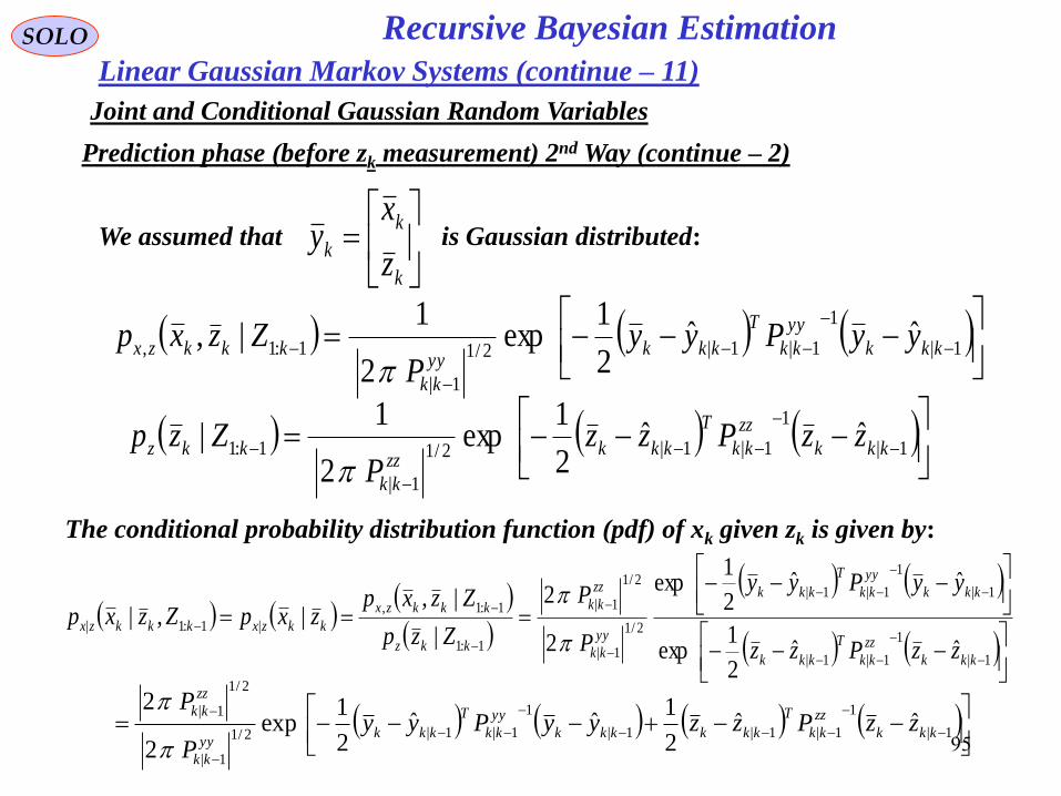
95
1|
1
1|1|2/1
1|
1:1,ˆˆ
2
1exp
2
1|, kkk
yy
kk
T
kkkyy
kk
kkkzx yyPyyP
Zzxp
Recursive Bayesian EstimationSOLO
Joint and Conditional Gaussian Random Variables
The conditional probability distribution function (pdf) of xk given zk is given by:
Prediction phase (before zk measurement) 2nd Way (continue – 2)
1|
1
1|1|2/1
1|
1:1ˆˆ
2
1exp
2
1| kkk
zz
kk
T
kkkzz
kk
kkz zzPzzP
Zzp
1|
1
1|1|
1|
1
1|1|
2/1
1|
2/1
1|
1:1
1:1,
|1:1|
ˆˆ2
1exp
ˆˆ2
1exp
2
2
|
|,|,|
kkk
zz
kk
T
kkk
kkk
yy
kk
T
kkk
yy
kk
zz
kk
kkz
kkkzx
kkzxkkkzx
zzPzz
yyPyy
P
P
Zzp
ZzxpzxpZzxp
1|
1
1|1|1|
1
1|1|2/1
1|
2/1
1|ˆˆ
2
1ˆˆ
2
1exp
2
2kkk
zz
kk
T
kkkkkk
yy
kk
T
kkkyy
kk
zz
kkzzPzzyyPyy
P
P
Linear Gaussian Markov Systems (continue – 11)
We assumed that is Gaussian distributed:
k
k
kz
xy

96
Recursive Bayesian EstimationSOLO
Joint and Conditional Gaussian Random Variables
Prediction phase (before zk measurement) 2nd Way (continue – 3)
1|
1
1|1|1|
1
1|1|2/1
1|
2/1
1|
|ˆˆ
2
1ˆˆ
2
1exp
2
2| kkk
zz
kk
T
kkkkkk
zz
kk
T
kkkyy
kk
zz
kk
kkzx zzPzzyyPyyP
Pzxp
Define: 1|1|ˆ:&ˆ: kkkkkkkk zzxx
k
zz
kk
T
kk
zz
kk
T
kk
zx
kk
T
kk
xz
kk
T
kk
xx
kk
T
k
kkkzz
T
k
k
k
zz
kk
zx
kk
xz
kk
xx
kk
T
k
k
k
zz
kk
T
k
k
k
zz
kk
zx
kk
xz
kk
xx
kk
T
k
k
kkk
zz
kk
T
kkkkkk
yy
kk
T
kkk
PTTTT
PTT
TT
PPP
PP
zzPzzyyPyyq
1
1|1|1|1|1|
1
1|
1|1|
1|1|
1
1|
1
1|1|
1|1|
1|
1
1|1|1|
1
1|1|ˆˆˆˆ:
Linear Gaussian Markov Systems (continue – 12)
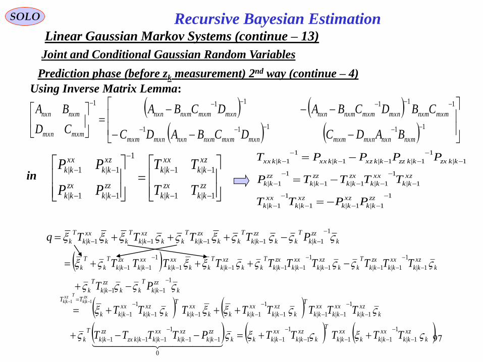
97
Recursive Bayesian EstimationSOLO
Joint and Conditional Gaussian Random Variables
Prediction phase (before zk measurement) 2nd way (continue – 4)
Using Inverse Matrix Lemma:
11111
111111
nxmnxnmxnmxmmxnmxmnxmnxnmxnmxm
mxmnxmmxnmxmnxmnxnmxnmxmnxmnxn
mxmmxn
nxmnxn
BADCDCBADC
CBDCBADCBA
CD
BA
zz
kk
zx
kk
xz
kk
xx
kk
zz
kk
zx
kk
xz
kk
xx
kk
TT
TT
PP
PP
1|1|
1|1|
1
1|1|
1|1|in
1
1|1|1|
1
1|
1|
1
1|1|1|
1
1|
1|
1
1|1|1|
1
1|
zz
kk
xz
kk
xz
kk
xx
kk
xz
kk
xx
kk
zx
kk
zz
kk
zz
kk
kkzxkkzzkkxzkkxxkkxx
PPTT
TTTTP
PPPPT
k
zz
kk
T
kk
zz
kk
T
kk
zx
kk
T
kk
xz
kk
T
kk
xx
kk
T
k PTTTTq 1
1|1|1|1|1|
k
zz
kk
T
kk
zz
kk
T
k
k
xz
kk
xx
kk
zx
kk
T
kk
xz
kk
xx
kk
zx
kk
T
kk
xz
kk
T
kk
xx
kk
xx
kk
zx
kk
T
k
T
k
PT
TTTTTTTTTT
1
1|1|
1|
1
1|1|1|
1
1|1|1|1|
1
1|1|
k
xz
kk
xx
kkk
xx
kk
T
k
xz
kk
xx
kkkk
zz
kk
xz
kk
xx
kkkkzx
zz
kk
T
k
k
xz
kk
xx
kk
xx
kk
T
k
xz
kk
xx
kkkk
xx
kk
T
k
xz
kk
xx
kkk
TT
TTTTTPTTTT
TTTTTTTT
zxkk
Txzkk
1|
1
1|1|1|
1
1|
0
1|1|
1
1|1|1|
1|
1
1|1|1|
1
1|1|1|
1
1|
1|1|
Linear Gaussian Markov Systems (continue – 13)
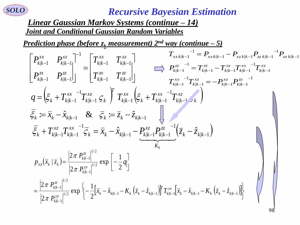
98
Recursive Bayesian EstimationSOLO
Joint and Conditional Gaussian Random Variables
Prediction phase (before zk measurement) 2nd way (continue – 5)
zz
kk
zx
kk
xz
kk
xx
kk
zz
kk
zx
kk
xz
kk
xx
kk
TT
TT
PP
PP
1|1|
1|1|
1
1|1|
1|1|
1
1|1|1|
1
1|
1|
1
1|1|1|
1
1|
1|
1
1|1|1|
1
1|
zz
kk
xz
kk
xz
kk
xx
kk
xz
kk
xx
kk
zx
kk
zz
kk
zz
kk
kkzxkkzzkkxzkkxxkkxx
PPTT
TTTTP
PPPPT
k
xz
kk
xx
kkk
xx
kk
T
k
xz
kk
xx
kkk TTTTTq 1|
1
1|1|1|
1
1|
1|1|ˆ:&ˆ: kkkkkkkk zzxx
1|1|1|1|1|2/1
1|
2/1
1|
2/1
1|
2/1
1|
|
ˆˆˆˆ2
1exp
2
2
2
1exp
2
2|
kkkkkkk
xx
kk
T
kkkkkkkyy
kk
zz
kk
yy
kk
zz
kk
kkzx
zzKxxTzzKxxP
P
qP
Pzxp
1|
1
1|1|1|
1
1|1|ˆˆ
kkk
K
zz
kk
xz
kkkkkk
xx
kk
xz
kkk zzPPxxTT
k
Linear Gaussian Markov Systems (continue – 14)

99
Recursive Bayesian EstimationSOLO
Joint and Conditional Gaussian Random Variables
Prediction phase (before zk measurement) 2nd Way (continue – 6)
1|
1
1|1|1|1|1|
1
1|1|1||ˆˆˆˆ
2
1exp| kkk
xx
kk
xz
kkkkk
xx
kk
T
kkk
xx
kk
xz
kkkkkkkzx zzPPxxTzzPPxxczxp
From this we can see that
1|
1
1|1|1||ˆˆˆ|
kkk
K
zz
kk
xz
kkkkkkkk zzPPxxzxE
k
T
k
zz
kkk
xx
kk
zx
kk
zz
kk
xz
kk
xx
kk
xx
kkk
T
kkkkkk
xx
kk
KPKP
PPPPTZxxxxEP
1|1|
1|
1
1|1|1|
1
1|:1|||ˆˆ
1|1:11|1|1|ˆˆ
kkk
T
kkkkkk
xx
kk PZxxxxEP
k
T
kkkkkk
T
kkkkkk
zz
kk SHPHRZzzzzEP :ˆˆ1|1:11|1|1|
T
kkkk
T
kkkkkk
xz
kk HPZzzxxEP 1|1:11|1|1|ˆˆ
Linear Gaussian Markov Systems (continue – 15)

100
Recursive Bayesian EstimationSOLO
Joint and Conditional Gaussian Random Variables
Prediction phase (before zk measurement) 2nd Way (continue – 7)
From this we can see that
111
1|1|
1
1|1|1||
kk
T
kkkkkk
T
kkkkk
T
kkkkkkk HRHPPHHPHRHPPP
1
1|
1
1|1|
1
1|1|
k
T
kkk
T
kkkkk
T
kkk
zz
kk
xz
kkk SHPHPHRHPPPK
Linear Gaussian Markov Systems (continue – 16)
kk
T
kkkkk KSKPP 1||
or
1|1:11|1|1|ˆˆ
kkk
T
kkkkkk
xx
kk PZxxxxEP
k
T
kkkkkk
T
kkkkkk
zz
kk SHPHRZzzzzEP :ˆˆ1|1:11|1|1|
T
kkkk
T
kkkkkk
xz
kk HPZzzxxEP 1|1:11|1|1|ˆˆ

101
We found that the optimal Kk is
1
1|1|
T
kkkkk
T
kkkk HPHRHPK
1111
|1
11
&
1
|1 11|
1
k
T
kkk
T
kkkkkk
LemmaMatrixInverse
existPR
T
kkkkk RHHRHPHRRHPHRkkk
1111
1|
1
1|
1
1|
k
T
kkk
T
kkkkk
T
kkkk
T
kkkk RHHRHPHRHPRHPK
1111
|1
111
|1|1
k
T
kkk
T
kkkkk
T
kkk
T
kkkkk RHHRHPHRHHRHPP
1
|
1111
|1
RHPRHHRHPK T
kkk
T
kkk
T
kkkk
If Rk-1 and Pk|k-1
-1 exist:
Recursive Bayesian EstimationSOLO
Linear Gaussian Markov Systems (continue – 17)
Relation Between 1st and 2nd ways
2nd Way
1st Way = 2nd Way

102
Recursive Bayesian EstimationSOLO
Closed-Form Solutions of Estimation
Closed-Form solutions for the Optimal Recursive Bayesian Estimation
can be derived only for special cases
The most important case:
• Dynamic and measurement models are linear
kkkk
kkkk
vuxkhz
wuxkfx
,,,
,,,1 111
kkkk
kkkkkkk
vxHz
wuGxx
111111
• Random noises are Gaussian
Qwwpw ,0;N
Rvvpv ,0;N
wQw
Qwp T
nw2
1exp
2
12/12/
vRv
Rvp T
pv
1
2/12/ 2
1exp
2
1
• Solution: KALMAN FILTER
• In other non-linear/non-Gaussian cases:
USE APPROXIMATIONS

103
Recursive Bayesian EstimationSOLO
Closed-Form Solutions of Estimation (continue – 1)
• Dynamic and measurement models are linear
kkkk
kkkkkkk
vxHz
wuGxx
111111
kv
kH kzkx
kx1 k
1kw1k
1kx
1ku 1kG
1zDelay
• The Optimal Estimator is the Kalman Filter
developed by R. E. Kalman in 1960
1|1|1|&1|:1| kkPkkekkeEkkxEkxkke x
T
xxx
lk
T
www kQlekeEkwEkwke ,
0
&:
lk
T
vvv kRlekeEkvEkvke ,
0
&: 0lekeE
T
vw
lk
lklk
1
0,
Rudolf E. Kalman
( 1920 - )
• K.F. is an Optimal Estimator (in the
Minimum Mean Square Estimator (MMSE) sense if:
- state and measurement models are linear
- the random elements are Gaussian
• Under those conditions, the covariance matrix:
- independent of the state (can be calculated off-line)
- equals the Cramer – Rao lower bound

104
Kalman Filter
State Estimation in a Linear System (one cycle)SOLO
1|1
1|1ˆ
kk
kk
P
x
1ktkt
T
t1|
1|ˆ
kk
kk
P
x
kk
kk
P
x
|
|ˆ
1: kk
Initialization TxxxxEPxEx 00000|000ˆˆˆ 0
State vector prediction111|111|ˆˆ
kkkkkkk uGxx1
Covariance matrix extrapolation111|111| k
T
kkkkkk QPP2
Innovation Covariancek
T
kkkkk RHPHS 1|3
Gain Matrix Computation1
1|
k
T
kkkk SHPK4
Measurement & Innovation1|ˆ
1|ˆ
kkz
kkkkk xHzi5
Filteringkkkkkk iKxx 1||
ˆˆ6
Covariance matrix updating
T
kkk
T
kkkkkk
kkkk
T
kkkkk
kkkk
T
kkkkkkk
KRKHKIPHKI
PHKI
KSKP
PHSHPPP
1|
1|
1|
1|
1
1|1||7

105
Kalman Filter
State Estimation in a Linear System (one cycle)Sensor Data
Processing and
Measurement
Formation
Observation -
to - Track
Association
Input
Data Track Maintenance
( Initialization,
Confirmation
and Deletion)
Filtering and
Prediction
Gating
Computations
Samuel S. Blackman, " Multiple-Target Tracking with Radar Applications", Artech House,
1986Samuel S. Blackman, Robert Popoli, " Design and Analysis of Modern Tracking Systems",
Artech House, 1999
SOLO
Evolution
of the system
(true state)
Estimation
of the state
State
Covariance
and
Kalman Filter
Computations
Controller
1kt
1|1ˆ
kkx
1kx
kkP |
2|1 kkP
kkx |ˆ
kx
1|1 kkP
1| kkP
1|ˆ
kkx
1kt kt
Real Trajectory
Estimated
Trajectory
Time
kt
Measurement at tk
kkkk vxHz
State Prediction
at tk
111|111|
ˆˆ kkkkkkk uGxx
State
Estimation
at tk-1
1|1ˆ
kkx
Control at tk-1
1ku
State Error Covariance
at tk-1
1|111|111|1ˆˆ
kkk
T
kkkkk xxxxEP
State Prediction
Covariance at tkk k
111|111| k
T
kkkkkk QPP
Innovation Covariance
k
T
kkkkk RHPHS 1|
Kalman Filter Gain
1
1|
k
T
kkkk SHPK
Update State
Covariance at tkk kT
kkkkkkk KSKPP 1||
Update State
Estimation at t k
kkkkkk Kxx 1||ˆˆ
Measurement Prediction
at tk
1|1|ˆˆ
kkkkk xHz
Transition to tk
11111 kkkkkk wuGxx
Innovation
1|ˆ
kkkk zz
State at tk-1
1kx
I.C.: 00|0ˆ xEx T
xxxxEP 0|000|000|0ˆˆ I.C.:
Rudolf E. Kalman
( 1920 - )

106
1|1|ˆˆ: kkkkkkkk zzxHzi
Recursive Bayesian EstimationSOLO
Linear Gaussian Markov Systems (continue – 18)
Innovation in a Kalman Filter
The innovation is the quantity:
We found that:
0ˆ||ˆ| 1|1:11:11|1:1 kkkkkkkkkk zZzEZzzEZiE
k
T
kkkkkk
T
kkk
T
kkkkkk SHPHRZiiEZzzzzE :ˆˆ1|1:11:11|1|
Using the smoothing property of the expectation:
xEdxxpxdxdyyxpx
dxdyypyxpxdyypdxyxpxyxEE
x
X
x y
YX
x yyxp
YYX
y
Y
x
YX
YX
,
||
,
,
||
,
1:1 k
T
jk
T
jk ZiiEEiiEwe have:
Assuming, without loss of generality, that k-1 ≥ j, and innovation i (j) is
independent on Z1:k-1, and it can be taken outside the inner expectation:
0
0
1:11:1
T
jkkk
T
jk
T
jk iZiEEZiiEEiiE
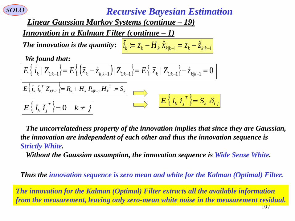
107
1|1|ˆˆ: kkkkkkkk zzxHzi
Recursive Bayesian EstimationSOLO
Linear Gaussian Markov Systems (continue – 19)
Innovation in a Kalman Filter (continue – 1)
The innovation is the quantity:
We found that:
0ˆ||ˆ| 1|1:11:11|1:1 kkkkkkkkkk zZzEZzzEZiE
k
T
kkkkkk
T
kk SHPHRZiiE :1|1:1
jkiiET
jk 0 jik
T
jk SiiE
The uncorrelatedness property of the innovation implies that since they are Gaussian,
the innovation are independent of each other and thus the innovation sequence is
Strictly White.
Without the Gaussian assumption, the innovation sequence is Wide Sense White.
Thus the innovation sequence is zero mean and white for the Kalman (Optimal) Filter.
The innovation for the Kalman (Optimal) Filter extracts all the available information
from the measurement, leaving only zero-mean white noise in the measurement residual.

108
kk
T
kn iSiz
1
:2
Recursive Bayesian EstimationSOLO
Linear Gaussian Markov Systems (continue – 20)
Innovation in a Kalman Filter (continue – 2)
Define the quantity:
Let use:kkk iSu
2/1
:
Since is Gaussian (a linear combination of the nz components of )
is Gaussian too with:ki ku ki
0:
0
2/1
kkk iESuE z
k
nk
S
T
kkkk
T
kkk
T
kk ISiiESSiiSEuuE 2/12/12/12/1
:
where Inz is the identity matrix of size nz. Therefore, since the covariance matrix of
u is diagonal, its components ui are uncorrelated and, since they are jointly Gaussian
they are also independent.
1,0;Pr:1
22 1
ii
n
i
ik
T
kkk
T
kn uuuuuiSiz
zN
Therefore is chi-square distributed with nz degrees of freedom.2
zn
Since Sk is symmetric and positive definite, it can be written as:
0,,& 1 SiSSkn
H
kk
H
kkkkznz
diagDITTTDTS H
kkkk TDTS11
2/12/1
1
2/12/12/1,,&
znSSk
H
kkkk diagDTDTS
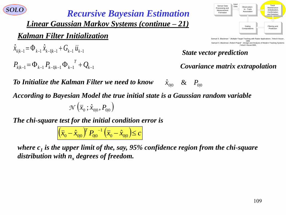
109
Sensor Data
Processing and
Measurement
Formation
Observation -
to - Track
Association
Input
DataTrack
Maintenance
) Initialization,
Confirmation
and Deletion(
Filtering and
Prediction
Gating
Computations
Samuel S . Blackman , " Multiple-Target Tracking with Radar Applications ", Artech House ,
1986Samuel S . Blackman , Robert Popoli , " Design and Analysis of Modern Tracking Systems
", Artech House , 1999
SOLO
Kalman Filter Initialization
State vector prediction111|111|ˆˆ
kkkkkkk uGxx
Covariance matrix extrapolation111|111| k
T
kkkkkk QPP
To Initialize the Kalman Filter we need to know 0|00|0 &ˆ Px
According to Bayesian Model the true initial state is a Gaussian random variable
0|00|00 ,ˆ; PxxN
The chi-square test for the initial condition error is
cxxPxxT
0|00
1
0|00|00ˆˆ
where c1 is the upper limit of the, say, 95% confidence region from the chi-square
distribution with nx degrees of freedom.
Recursive Bayesian EstimationLinear Gaussian Markov Systems (continue – 21)

110
SOLO
Return to Table of Content
can be estimated using at least two measurements 0|0&0|0ˆ Px
From the first measurement, z1, using Least Square we obtain 1
111
1 zRHHRHx TT
From the second measurement
1|222111|2ˆˆ&ˆˆ xHzxx Predictions before the second measurement
RHPHST 21|222
The Preliminary Track Gate used for the second measurement is determined from the
worst-case target conditions including maneuver and data miscorrelations.
Sensor Data
Processing and
Measurement
Formation
Observation -
to - Track
Association
Input
DataTrack
Maintenance
(Initialization,
Confirmation
and Deletion)
Filtering and
Prediction
Gating
Computations
Samuel S . Blackman , " Multiple-Target Tracking with Radar Applications ", Artech House ,
1986Samuel S . Blackman , Robert Popoli , " Design and Analysis of Modern Tracking Systems
", Artech House , 1999
Kalman Filter Initialization
Linear Gaussian Markov Systems (continue – 22)
Recursive Bayesian Estimation

111
SOLO
Return to Table of Content
Strategies for Kalman Filter Initialization (First Step)
Sensor Data
Processing and
Measurement
Formation
Observation -
to - Track
Association
Input
DataTrack
Maintenance
(Initialization,
Confirmation
and Deletion)
Filtering and
Prediction
Gating
Computations
Samuel S . Blackman , " Multiple-Target Tracking with Radar Applications ", Artech House ,
1986Samuel S . Blackman , Robert Popoli , " Design and Analysis of Modern Tracking Systems
", Artech House , 1999
MaxVT
2
MaxT
2
MaxT
MaxVT
2
MaxT
2
MaxT
minVT
MaxVT
minVT
MaxVT
MAX SPEED and
TURNING RATE
SPECIFIED
MAX, MIN SPEED
and
TURNING RATE
SPECIFIED
MAX SPEED
SPECIFIED
MAX, MIN SPEED
SPECIFIED
Kalman Filter Initialization
Linear Gaussian Markov Systems (continue – 23)
Recursive Bayesian Estimation

112
SOLO
Information Kalman FilterFor some applications (such as bearing only tracking) the initial state covariance
matrix P0|0 may be very large. As a result the Kalman Filter formulation can encounter
numerical problems.
For those cases is better to use a formulation with P0|0-1.
kk
T
kkkkk HRHPP11
1|
1
|
Start with:
1
|
k
T
kkkk RHPK
1
1
11
1|1
1
1
1
1
1
1
1
11|1
1
1|
kkkk
T
kkk
T
kkk
LemmaMatrixInverse
k
T
kkkkkk
QPQQQ
QPP
111
1|
1111
1|
1
kkkk
T
kkk
T
kkk
LemmaMatrixInverse
k
T
kkkkk RHPHRHHRRRHPHS
First Version: Change only the Covariance Matrices Computations
Linear Gaussian Markov Systems (continue – 24)
Recursive Bayesian Estimation

113
Sensor Data
Processing and
Measurement
Formation
Observation -
to - Track
Association
Input
Data Track Maintenance
( Initialization,
Confirmation
and Deletion)
Filtering and
Prediction
Gating
Computations
Samuel S. Blackman, " Multiple-Target Tracking with Radar Applications", Artech House,
1986Samuel S. Blackman, Robert Popoli, " Design and Analysis of Modern Tracking Systems",
Artech House, 1999
SOLO
Evolution
of the system
(true state)
Estimation
of the state
State
Covariance
and
Kalman Filter
Computations
Controller
1kt
1|1ˆ
kkx
1kx
kkP |
2|1 kkP
kkx |ˆ
kx
1|1 kkP
1| kkP
1|ˆ
kkx
1kt kt
Real Trajectory
Estimated
Trajectory
Time
kt
Measurement at tk
kkkk vxHz
State Prediction
at tk
111|111|
ˆˆ kkkkkkk uGxx
Control at tk-1
1ku
State Error Covariance
at tk-1
1
1|111|11
1
1|1
ˆˆ
kkk
T
kkk
kk
xxxxE
P
State Prediction
Covariance at tkk k
1
11
11
1|11
1
111
1
1
1
1
1
1|
k
T
kkkkk
T
kkk
kkk
QPQQ
QP
Innovation Covariance
111
1|
11
11
k
T
kkkkk
T
kkk
kk
RHPHRHHR
RS
Kalman Filter Gain
1
|
k
T
kkkk RHPK
Update State
Covariance at tkk k
kk
T
kkkkk HRHPP11
1|
1
|
Update State
Estimation at t k
kkkkkk iKxx 1||ˆˆ
Measurement Prediction
at tk
1|1|ˆˆ
kkkkk xHz
Transition to tk
11111 kkkkkk wuGxx
Innovation
1|ˆ
kkkk zz
State Estimation
at tk-1
1|1
ˆ kkx
State at tk-1
1kx
I.C.: 00|0ˆ xEx T
xxxxEP 0|000|000|0ˆˆ I.C.:
Rudolf E. Kalman
( 1920 - )
Information Kalman Filter
Version 1

114
SOLO
For some applications (such as bearing only tracking)
the initial state covariance matrix P0|0 may be very
large. As a result the Kalman Filter formulation can encounter numerical problems.
For those cases is better to use a formulation with P0|0-1.
kk
T
kkkkk HRHPP11
1|
1
|
1
|
k
T
kkkk RHPK
Start with: 1
11|1
1
1|
k
T
kkkkkk QPP
111
1|
1111
1|
1
kkkk
T
kkk
T
kkkk
T
kkkkk RHPHRHHRRRHPHS
Define:
11
1|1
1
1|11|1|1
1
1|
kkk
T
k
T
kkkkkk
T
kkkkkk PPAPA
1|1|1|
11
11|1|
1|
11
11|1|1|
1
1
1
1|
1
1|
1|
kkkkkk
B
kkkkk
kkkkkkkkk
LemmaMatrixInverse
kkkkk
ABIAQAAI
AQAAAQAP
kk
Second Version: Change both the Covariance Matrices and Filter States Computations
Information Kalman Filter
Linear Gaussian Markov Systems (continue – 24)
Recursive Bayesian Estimation
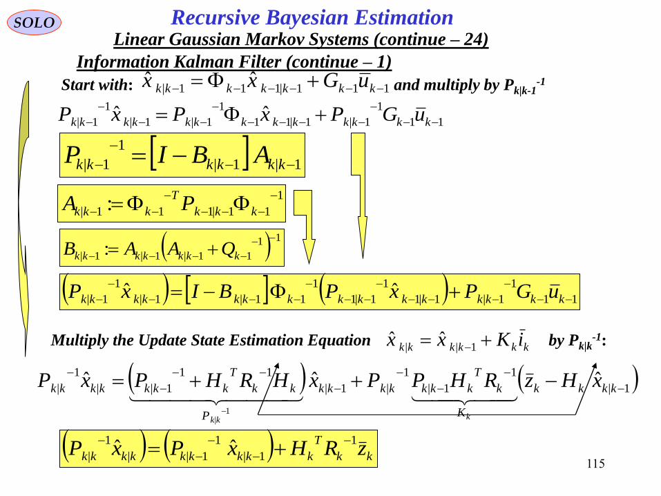
115
SOLO
111|111|ˆˆ
kkkkkkk uGxxStart with: and multiply by Pk|k-1-1
1
11|111| :
kkk
T
kkk PA
1|
1
1|
1
|1|
11
1||
1
|ˆˆˆ
1|
kkkk
K
k
T
kkkkkkk
P
kk
T
kkkkkkk xHzRHPPxHRHPxP
kkk
kk
T
kkkkkkkkk zRHxPxP1
1|
1
1||
1
|ˆˆ
11
1
1|1|11
1
1|1|
1
1|ˆˆ
kkkkkkkkkkkkk uGPxPxP
1|1|
1
1|
kkkkkk ABIP
11
1
1|1|1
1
1|1
1
11|1|
1
1|ˆˆ
kkkkkkkkkkkkkkk uGPxPBIxP
11
11|1|1| :
kkkkkkk QAAB
Multiply the Update State Estimation Equation by Pk|k-1:
kkkkkk iKxx 1||ˆˆ
Information Kalman Filter (continue – 1)
Linear Gaussian Markov Systems (continue – 24)
Recursive Bayesian Estimation

116
Sensor Data
Processing and
Measurement
Formation
Observation -
to - Track
Association
Input
Data Track Maintenance
( Initialization,
Confirmation
and Deletion)
Filtering and
Prediction
Gating
Computations
Samuel S. Blackman, " Multiple-Target Tracking with Radar Applications", Artech House,
1986Samuel S. Blackman, Robert Popoli, " Design and Analysis of Modern Tracking Systems",
Artech House, 1999
SOLO
Evolution
of the system
(true state)
Estimation
of the state
State
Covariance
and
Kalman Filter
Computations
Controller
1kt
1|1ˆ
kkx
1kx
kkP |
2|1 kkP
kkx |ˆ
kx
1|1 kkP
1| kkP
1|ˆ
kkx
1kt kt
Real Trajectory
Estimated
Trajectory
Time
kt
Measurement at tk
kkkk vxHz
State Prediction
at tk
11
1
1|
1|1
1
1|1
1
11|1|
1
1|ˆˆ
kkkk
kkkkkkkkkkk
uGP
xPBIxP
Control at tk-1
1ku
State Error Covariance
at tk-1
1
1|111|11
1
1|1
ˆˆ
kkk
T
kkk
kk
xxxxE
P
State PredictionCovariance at tkk k
1
11|1|1|
1
1
1
1|111|
1|1|
1
1|
kkkkkkk
kkk
T
kkk
kkkkkk
QAAB
PA
ABIP
Innovation Covariance
111
1|
11
11
k
T
kkkkk
T
kkk
kk
RHPHRHHR
RS
Kalman Filter Gain
1
|
k
T
kkkk RHPK
Update State
Covariance at tkk k
kk
T
kkkkk HRHPP11
1|
1
|
Update State
Estimation at t k
kkkkkkkkkkk zRHxPxP1
1|
1
1||
1
|ˆˆ
Measurement Prediction
at tk
1|1|ˆˆ
kkkkk xHz
Transition to tk
11111 kkkkkk wuGxx
Innovation
1|ˆ
kkkk zz
State Estimation
at tk-1
1|11|1
ˆ kkkk xP
State at tk-1
1kx
I.C.: 00|0ˆ xEx T
xxxxEP 0|000|000|0ˆˆ I.C.:
Rudolf E. Kalman
( 1920 - )
Information Kalman Filter
(Version 2)
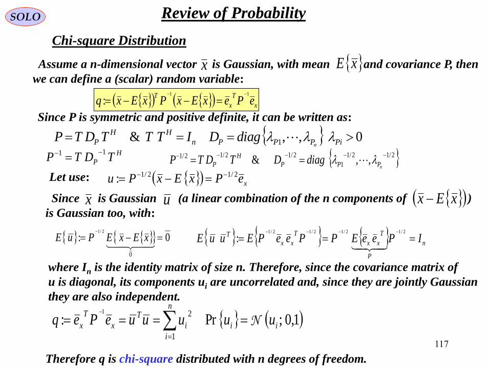
117
SOLO Review of Probability
Chi-square Distribution
x
T
x
TePexExPxExq
11
:
Assume a n-dimensional vector is Gaussian, with mean and covariance P, then
we can define a (scalar) random variable:x xE
Since P is symmetric and positive definite, it can be written as:
0,,& 1 PiPPPn
HH
P ndiagDITTTDTP
H
P TDTP11 2/12/1
1
2/12/12/1 ,,&
nPPP
H
P diagDTDTP
Since is Gaussian (a linear combination of the n components of )
is Gaussian too, with:x u xEx
0:
0
2/1
xExEPuE n
P
T
xx
T
xx
T IPeeEPPeePEuuE 2/12/12/12/1
:
where In is the identity matrix of size n. Therefore, since the covariance matrix of
u is diagonal, its components ui are uncorrelated and, since they are jointly Gaussian
they are also independent.
1,0;Pr:1
21
ii
n
i
i
T
x
T
x uuuuuePeq N
Therefore q is chi-square distributed with n degrees of freedom.
Let use: xePxExPu 2/12/1:
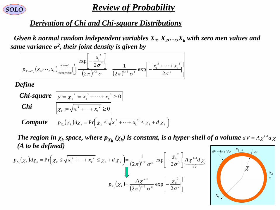
118
SOLO Review of Probability
Derivation of Chi and Chi-square Distributions
Given k normal random independent variables X1, X2,…,Xk with zero men values and
same variance σ2, their joint density is given by
2
22
1
2/1
2/1
2
2
12
exp2
1
2
2exp
,,1
k
kk
k
i
i
normal
tindependenkXX
xx
x
xxpk
Define
Chi-square 0::22
1
2
kkxxy
Chi 0:22
1
kkxx
kkkkkkdxxdp
k
22
1Pr
The region in χk space, where pΧk(χk) is constant, is a hyper-shell of a volume
(A to be defined)
dAVd k 1
Vd
kk
kkkkkkkkdAdxxdp
k
1
2
2
2/
22
12
exp2
1Pr
2
2
2/
1
2exp
2
k
kk
k
k
Ap
k
Compute
1x
2x
3x
d ddV 24

119
SOLO Review of Probability
Derivation of Chi and Chi-square Distributions (continue – 1)
k
k
kk
k
kU
Ap
k
2
2
2/
1
2exp
2
Chi-square 0:22
1
2
kkxxy
00
02
exp22
1 2
2/1
2/
0
2
2
2
y
yy
yy
A
ypyp
d
ydypp
k
kk
y
k
Yk kkk
A is determined from the condition 1
dyypY
2/
212/
222exp
22
2/
2/20
2
2
2
22/k
AkAy
dyyA
dyyp
k
k
k
kY
yUyy
kkyp
kk
Y
2
2/2
2
2/
2exp
2/
2/1,;
Γ is the gamma function
0
1 exp dttta a
k
k
k
k
k
k
kU
kp
k
2
212/2
2exp
2/
2/1
00
01:
a
aaU
Function of
One Random
Variable
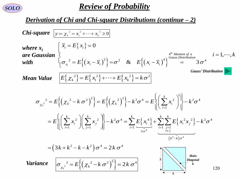
120
SOLO Review of Probability
Derivation of Chi and Chi-square Distributions (continue – 2)
Chi-square 0:22
1
2
kkxxy
Mean Value 2 2 2 2
1k kE E x E x k
4
2 42 2 4
0
1, ,
& 3
th
i
i i
Moment of aGauss Distribution
x i i i i
x E x
i k
E x x E x x
2
4
2 4
22 2
2 2 2 2 2 4 2 2 4
1
2 2 2 4 4 2 2 2 4
1 1 1 1 1
3
2 2 4 43 2
k
k
k k i
i
k k k k k
i j i i j
i j i i ji j
k k
E k E k E x k
E x x k E x E x x k
k k k k k
k
kMain
Diagonal
kVariance 2
22 2 2 42
kkE k k
where xi
are Gaussian
with
Gauss’ Distribution

121
SOLO Review of ProbabilityDerivation of Chi and Chi-square Distributions (continue – 3)
Tail probabilities of the chi-square and normal densities.
The Table presents the points on the chi-square
distribution for a given upper tail probability
xyQ Pr
where y = χn2 and n is the number of degrees
of freedom. This tabulated function is also
known as the complementary distribution.
An alternative way of writing the previous
equation is: QxyQ n 1Pr12
which indicates that at the left of the point x
the probability mass is 1 – Q. This is
100 (1 – Q) percentile point.
Examples
1. The 95 % probability region for χ22 variable
can be taken at the one-sided probability
region (cutting off the 5% upper tail): 99.5,095.0,02
2
5.99
2. Or the two-sided probability region (cutting off both 2.5% tails): 38.7,05.0975.0,025.02
2
2
2
0.51
0.975 0.0250.05
7.38
3. For χ1002 variable, the two-sided 95% probability region (cutting off both 2.5% tails) is:
130,74975.0,025.02
100
2
100
74130
Run This

122
SOLO Review of Probability
Derivation of Chi and Chi-square Distributions (continue – 4)
Note the skewedness of the chi-square
distribution: the above two-sided regions are
not symmetric about the corresponding means
nE n 2
Tail probabilities of the chi-square and normal densities.
For degrees of freedom above 100, the
following approximation of the points on the
chi-square distribution can be used:
22121
2
11 nQQn G
where G ( ) is given in the last line of the Table
and shows the point x on the standard (zero
mean and unity variance) Gaussian distribution
for the same tail probabilities.
In the case Pr { y } = N (y; 0,1) and with
Q = Pr { y>x }, we have x (1-Q) :=G (1-Q)
5.990.51
0.975 0.0250.05
7.38
Return to Table of Content
Run This
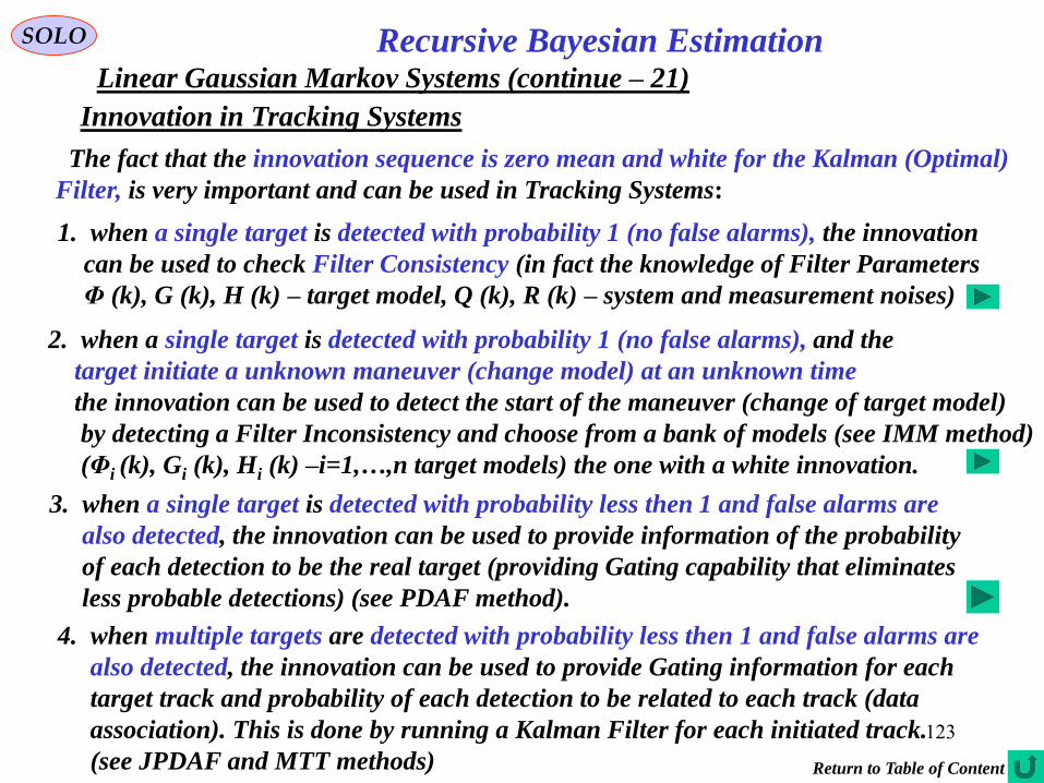
123
Recursive Bayesian EstimationSOLO
Linear Gaussian Markov Systems (continue – 21)
Innovation in Tracking Systems
The fact that the innovation sequence is zero mean and white for the Kalman (Optimal)
Filter, is very important and can be used in Tracking Systems:
1. when a single target is detected with probability 1 (no false alarms), the innovation
can be used to check Filter Consistency (in fact the knowledge of Filter Parameters
Φ (k), G (k), H (k) – target model, Q (k), R (k) – system and measurement noises)
4. when multiple targets are detected with probability less then 1 and false alarms are
also detected, the innovation can be used to provide Gating information for each
target track and probability of each detection to be related to each track (data
association). This is done by running a Kalman Filter for each initiated track.
(see JPDAF and MTT methods) Return to Table of Content
2. when a single target is detected with probability 1 (no false alarms), and the
target initiate a unknown maneuver (change model) at an unknown time
the innovation can be used to detect the start of the maneuver (change of target model)
by detecting a Filter Inconsistency and choose from a bank of models (see IMM method)
(Φi (k), Gi (k), Hi (k) –i=1,…,n target models) the one with a white innovation.
3. when a single target is detected with probability less then 1 and false alarms are
also detected, the innovation can be used to provide information of the probability
of each detection to be the real target (providing Gating capability that eliminates
less probable detections) (see PDAF method).

124
Recursive Bayesian EstimationSOLO
Linear Gaussian Markov Systems (continue – 22)
Evaluation of Kalman Filter Consistency
A state-estimator (filter) is called consistent if its state estimation error satisfy
0|~:|ˆ kkxEkkxkxE
kkPkkxkkxEkkxkxkkxkxE TT||~|~:|ˆ|ˆ
this is a finite-sample consistency property, that is, the estimation errors based on a
finite number of samples (measurements) should be consistent with the theoretical
statistical properties:
• Have zero mean (i.e. the estimates are unbiased).
• Have covariance matrix as calculated by the Filter.
The Consistency Criteria of a Filter are:
1. The state errors should be acceptable as zero mean and have magnitude commensurate
with the state covariance as yielded by the Filter.
2. The innovation should have the same property as in (1).
3. The innovation should be white noise.
Only the last two criteria (based on innovation) can be tested in real data applications.
The first criterion, which is the most important, can be tested only in simulations.

125
Recursive Bayesian EstimationSOLO
Linear Gaussian Markov Systems (continue – 23)
Evaluation of Kalman Filter Consistency (continue – 1)
When we design the Kalman Filter, we can perform Monte Carlo (N independent runs)
Simulations to check the Filter Consistency (expected performances).
Real time (Single-Run Tests)
In Real Time, we can use a single run (N = 1). In this case the simulations are replaced
by assuming that we can replace the Ensemble Averages (of the simulations) by the
Time Averages based on the Ergodicity of the Innovation and perform only the tests
(2) and (3) based on Innovation properties.
The Innovation bias and covariance can be evaluated using
K
k
TK
k
kikiK
SkiK
i11 1
1ˆ&1ˆ

126
Recursive Bayesian EstimationSOLO
Linear Gaussian Markov Systems (continue – 24)
Evaluation of Kalman Filter Consistency (continue – 2)
Real time (Single-Run Tests) (continue – 1)
Test 2: kSkikiEkiEkkzkzE T &0:1|ˆ
Using the Time-Average Normalized Innovation
Squared (NIS) statistics
K
k
T
i kikSkiK 1
11:
must have a chi-square distribution with
K nz degrees of freedom.iK
Tail probabilities of the chi-square and normal densities.
The test is successful if 21, rri
where the confidence interval [r1,r2] is defined
using the chi-square distribution of i
1,Pr 21 rri
For example for K=50, nz=2, and α=0.05, using the two
tails of the chi-square distribution we get
6.250/130130925.0
5.150/7474025.0~50
2
2
100
1
2
1002
100
r
ri
0.9750.025
74130
Run This

127
Recursive Bayesian EstimationSOLO
Linear Gaussian Markov Systems (continue – 25)
Evaluation of Kalman Filter Consistency (continue – 3)
Real time (Single-Run Tests) (continue – 2)
Test 3: Whiteness of Innovation
Use the Normalized Time-Average Autocorrelation
2/1
111
:
K
k
TK
k
TK
k
T
i lkilkikikilkikil
In view of the Central Limit Theorem, for large K, this statistics is normal distributed.
For l≠0 the variance can be shown to be 1/K that tends to zero for large K.
Denoting by ξ a zero-mean unity-variance normal
random variable, let r1 such that
1,Pr 11 rr
For α=0.05, will define (from the normal distribution)
r1 = 1.96. Since has standard deviation of
The corresponding probability region for α=0.05 will
be [-r, r] where
i K/1
KKrr /96.1/1 Normal Distribution

128
Recursive Bayesian EstimationSOLO
Linear Gaussian Markov Systems (continue – 26)
Evaluation of Kalman Filter Consistency (continue – 4)
Monte-Carlo Simulation Based Tests
The tests will be based on the results of Monte-Carlo Simulations (Runs) that provide
N independent samples
NikkxkkxEkkPkkxkxkkxT
iiiii ,,1|~|~|&|ˆ:|~
Test 1:
For each run i we compute at each scan k
And compute the Normalized (state) Estimation Error Squared (NEES)
NikkxkkPkkxk i
T
ixi ,,1|~||~: 1
Under the Hypothesis that the Filter is Consistent and the Linear Gaussian,
is chi-square distributed with nx (dimension of x) degrees of freedom.
Then
kxi
xxi nkE
The average, over N runs, of is kxi
N
i
xix kN
k1
1:
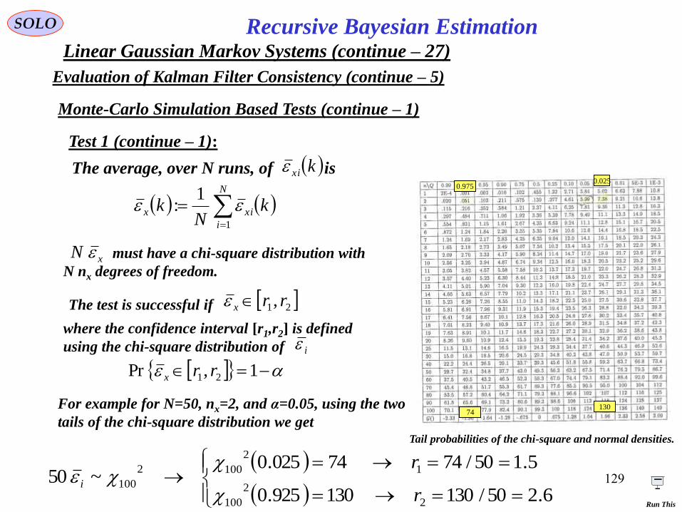
129
Recursive Bayesian EstimationSOLO
Linear Gaussian Markov Systems (continue – 27)
Evaluation of Kalman Filter Consistency (continue – 5)
Monte-Carlo Simulation Based Tests (continue – 1)
Test 1 (continue – 1):
The average, over N runs, of is kxi
N
i
xix kN
k1
1:
The test is successful if 21, rrx
where the confidence interval [r1,r2] is defined
using the chi-square distribution of i
1,Pr 21 rrx
For example for N=50, nx=2, and α=0.05, using the two
tails of the chi-square distribution we get
6.250/130130925.0
5.150/7474025.0~50
2
2
100
1
2
1002
100
r
ri
Tail probabilities of the chi-square and normal densities.
0.9750.025
74130
must have a chi-square distribution with
N nx degrees of freedom.xN
Run This

130
Recursive Bayesian EstimationSOLO
Linear Gaussian Markov Systems (continue – 28)
Evaluation of Kalman Filter Consistency (continue – 6)
Monte-Carlo Simulation Based Tests (continue – 2)
The test is successful if 21, rri
where the confidence interval [r1,r2] is defined
using the chi-square distribution of i
1,Pr 21 rri
For example for N=50, nz=2, and α=0.05, using the two
tails of the chi-square distribution we get
6.250/130130925.0
5.150/7474025.0~50
2
2
100
1
2
1002
100
r
ri
Tail probabilities of the chi-square and normal densities.
0.9750.025
74130
must have a chi-square distribution with
N nz degrees of freedom.iN
Test 2: kSkikiEkiEkkzkzE T &0:1|ˆ
Using the Normalized Innovation Squared (NIS)
statistics, compute from N Monte-Carlo runs:
N
j
jj
T
ji kikSkiN
k1
11:

131
Recursive Bayesian EstimationSOLO
Linear Gaussian Markov Systems (continue – 29)
Evaluation of Kalman Filter Consistency (continue – 7)
Test 3: Whiteness of Innovation
Use the Normalized Sample Average Autocorrelation
2/1
111
:,
N
j
j
T
j
N
j
j
T
j
N
j
j
T
ji mimikikimikimk
In view of the Central Limit Theorem, for large N, this statistics is normal distributed.
For k≠m the variance can be shown to be 1/N that tends to zero for large N.
Denoting by ξ a zero-mean unity-variance normal
random variable, let r1 such that
1,Pr 11 rr
For α=0.05, will define (from the normal distribution)
r1 = 1.96. Since has standard deviation of
The corresponding probability region for α=0.05 will
be [-r, r] where
i N/1
NNrr /96.1/1 Normal Distribution
Monte-Carlo Simulation Based Tests (continue – 3)

132
Recursive Bayesian EstimationSOLO
Linear Gaussian Markov Systems (continue – 30)
Evaluation of Kalman Filter Consistency (continue – 8)
Examples Bar-Shalom, Y, Li, X-R, “Estimation and Tracking: Principles, Techniques
and Software”, Artech House, 1993, pg.242
Monte-Carlo Simulation Based Tests (continue – 4)
Single Run, 95% probability
99.5,0xTest (a) Passes if
A one-sided region is considered.
For nx = 2 we have
99.5,095.0,02 2
2
2
2 xn
K
k
T
x kkxkkPkkxK
k1
1 |~||~1:
qkxkkx 1
See behavior of for various values of the process noise q
for filters that are perfectly matched.

133
Recursive Bayesian EstimationSOLO
Linear Gaussian Markov Systems (continue – 31)
Evaluation of Kalman Filter Consistency (continue – 9)
Examples Bar-Shalom, Y, Li, X-R, “Estimation and Tracking: Principles, Techniques
and Software”, Artech House, 1993, pg.244
Monte-Carlo Simulation Based Tests (continue – 5)
Monte-Carlo, N=50, 95% probability
6.2,5.150/130,50/74 xTest (a) Passes if
N
j
jj
T
jx kkxkkPkkxN
k1
1|~||~1
:(a)
2/1
111
:,
N
j
j
T
j
N
j
j
T
j
N
j
j
T
ji mimikikimikimk(c)
The corresponding probability region for
α=0.05 will be [-r, r] where
28.050/96.1/1 Nrr
43.1,65.050/4.71,50/3.32 iTest (b) Passes if
N
j
jj
T
ji kikSkiN
k1
11:(b)
130,74925.0,025.02 2
100
2
100 xn
71,32925.0,025.01 2
100
2
100 zn
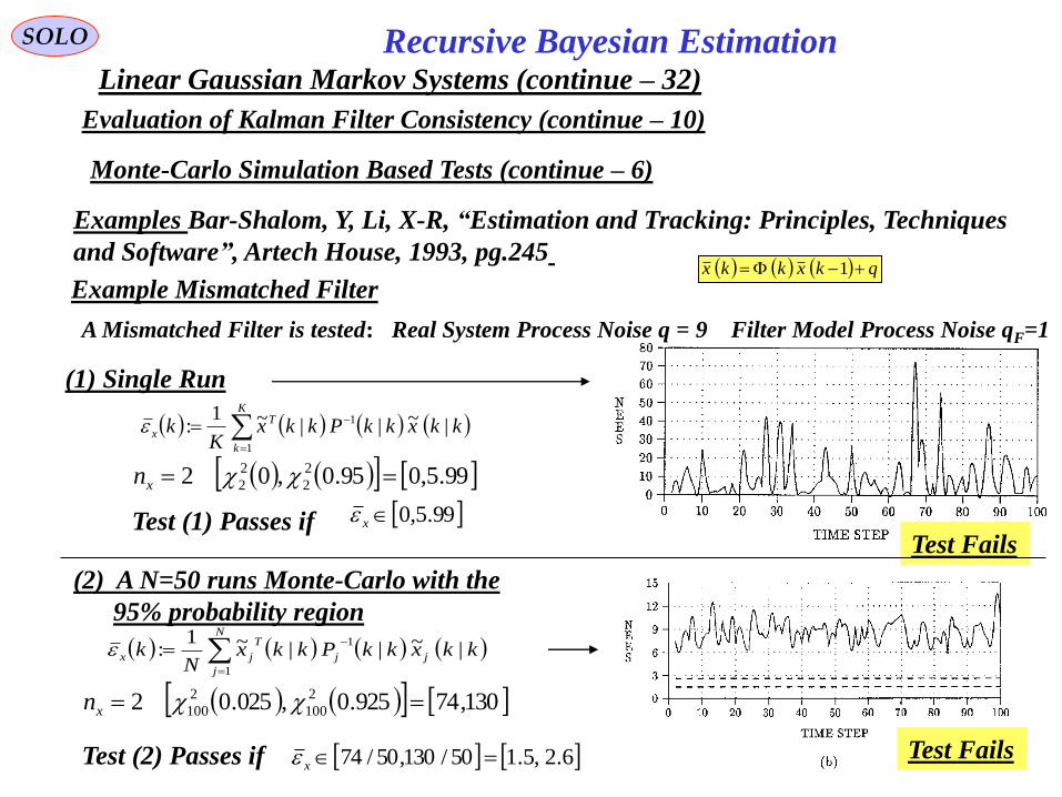
134
Recursive Bayesian EstimationSOLO
Linear Gaussian Markov Systems (continue – 32)
Evaluation of Kalman Filter Consistency (continue – 10)
Examples Bar-Shalom, Y, Li, X-R, “Estimation and Tracking: Principles, Techniques
and Software”, Artech House, 1993, pg.245
Monte-Carlo Simulation Based Tests (continue – 6)
Example Mismatched Filter
A Mismatched Filter is tested: Real System Process Noise q = 9 Filter Model Process Noise qF=1
K
k
T
x kkxkkPkkxK
k1
1 |~||~1:
qkxkkx 1
(1) Single Run
(2) A N=50 runs Monte-Carlo with the
95% probability region
N
j
jj
T
jx kkxkkPkkxN
k1
1|~||~1
:
6.2,5.150/130,50/74 xTest (2) Passes if
130,74925.0,025.02 2
100
2
100 xn
Test Fails
Test Fails
99.5,0xTest (1) Passes if
99.5,095.0,02 2
2
2
2 xn

135
Recursive Bayesian EstimationSOLO
Linear Gaussian Markov Systems (continue – 33)
Evaluation of Kalman Filter Consistency (continue – 11)
Examples Bar-Shalom, Y, Li, X-R, “Estimation and Tracking: Principles, Techniques
and Software”, Artech House, 1993, pg.246
Monte-Carlo Simulation Based Tests (continue – 7)
Example Mismatched Filter (continue -1)
A Mismatched Filter is tested: Real System Process Noise q = 9 Filter Model Process Noise qF=1
qkxkkx 1
(3) A N=50 runs Monte-Carlo with the
95% probability region
(4) A N=50 runs Monte-Carlo with the
95% probability region
N
j
jj
T
ji kikSkiN
k1
11:
43.1,65.050/4.71,50/3.32 iTest (3) Passes if
71,32925.0,025.01 2
100
2
100 zn
2/1
111
:,
N
j
j
T
j
N
j
j
T
j
N
j
j
T
ji mimikikimikimk
(c)
The corresponding probability region for
α=0.05 will be [-r, r] where
28.050/96.1/1 Nrr
Test Fails
Test Fails
Return to Table of Content
Innovation in Tracking

136
SOLO
Kalman Filter for Filtering Position and Velocity Measurements
Assume a Cartezian Model of a Non-maneuvering Target:
wx
x
x
x
td
d
wx
xx
BA
1
0
00
10
10
1
!
1
2
1exp: 22
0
TTAITA
nTATAIdAT nn
T
200
00
00
00
00
10
00
10
00
102
nAAA n
2
1
v
v
x
xvxz
Measurements
T
TTd
TdBTT
TTT
2/2/
1
0
10
1:
2
0
2
00
Discrete System
1111
1
kkkk
kkkkk
vxHz
wxx
kj
V
PT
jkkkk
H
k
kjq
T
jkkkkk
vvERvxz
wwEQwT
Tx
Tx
k
kk
2
2
111111
22
1
0
0&
10
01
&2/
10
1
1
Target Estimators
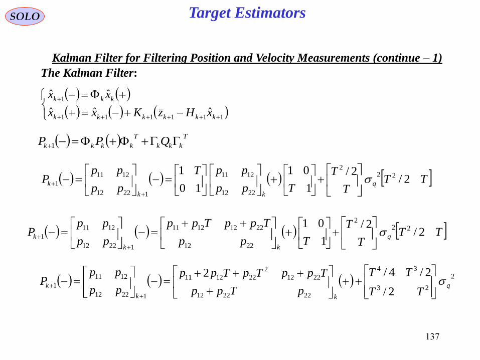
137
SOLO
Kalman Filter for Filtering Position and Velocity Measurements (continue – 1)
The Kalman Filter:
111111
1
ˆˆˆ
ˆˆ
kkkkkk
kkk
xHzKxx
xx
T
kkk
T
kkkk QPP 1
TTT
T
Tpp
ppT
pp
ppP q
kk
k 2/2/
1
01
10
122
2
2212
1211
12212
1211
1
TTT
T
Tpp
TppTpp
pp
ppP q
kk
k 2/2/
1
0122
2
2212
22121211
12212
1211
1
2
23
34
222212
2212
2
221211
12212
1211
12/
2/4/2q
kk
kTT
TT
pTpp
TppTpTpp
pp
ppP
Target Estimators
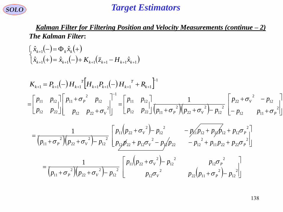
138
SOLO
Kalman Filter for Filtering Position and Velocity Measurements (continue – 2)
The Kalman Filter:
111111
1
ˆˆˆ
ˆˆ
kkkkkk
kkk
xHzKxx
xx
1
1111111
k
T
kkk
T
kkk RHPHHPK
2
1112
12
2
22
2
12
2
22
2
112212
1211
1
2
2212
12
2
11
2212
1211 1
P
V
VPV
P
pp
pp
ppppp
pp
pp
pp
pp
pp
2
222211
2
122212
2
122212
2
1212111211
2
12
2
2211
2
12
2
22
2
11
1
PV
PV
VP ppppppppp
pppppppp
ppp
2
12
2
1122
2
12
2
12
2
12
2
2211
2
12
2
22
2
11
1
pppp
pppp
pppPV
PV
VP
Target Estimators

139
SOLO
Kalman Filter for Filtering Position and Velocity Measurements (continue – 3)
The Kalman Filter:
1
1111111
k
T
kkk
T
kkk RHPHHPK
T
kkk
T
kkkkk
kkk
kKRKHKIPHKI
PHKIP
11111111
111
1
2
12
2
1122
2
12
2
12
2
12
2
2211
2
12
2
22
2
1112221
1211
1
1
pppp
pppp
pppKK
KKK
PV
PV
VPk
k
22
11
2
12
2
12
22
22
2
12
2
22
2
11
11
1
VPV
PPV
VP
kk
pp
pp
pppHKI
2212
1211
22
11
2
12
2
12
22
22
2
12
2
22
2
11
1111
1
pp
pp
pp
pp
pppPHKIP
VPV
PPV
VP
kkkk
2
2
12221
1211
1
2
22
2
21
2
12
2
11
2
1222
2
11
222
12
22
12
2
1211
2
22
2
2
12
2
22
2
11
1
0
0
1
V
P
k
kVP
VP
PVVP
VPVP
VP
k
KK
KK
KK
KK
pppp
pppp
pppP
Target Estimators

140
wx
x
x
x
td
d
BA
1
0
00
10
SOLO
We want to find the steady-state form of the filter for
Assume that only the position measurements are available
x
x
- position
- velocity
kjjkkk
k
kkkk RvvEvEvx
xvxHz
1111
1
1111 0&01
Discrete System
1111
1
kkkk
kkkkk
vxHz
wxx
kjP
T
jkkkk
H
k
kjw
T
jkkkkk
vvERvxz
wwEQwT
Tx
Tx
k
kk
2
111111
22
1
&01
&2/
10
1
1
α - β (2-D) Filter with Piecewise Constant White Noise Acceleration Model
Target Estimators

141
SOLO
Discrete System
1111
1
kkkk
kkkkk
vxHz
wxx
kjP
T
jkkkk
H
k
kjw
T
jkkkkk
vvERvxz
wwEQwT
Tx
Tx
k
kk
2
111111
22
1
&01
&2/
10
1
1
11/111 kRkHkkPkHkST
111/11
kSkHkkPkK T
When the Kalman Filter reaches the steady-state
2212
12111/1lim/lim
pp
ppkkPkkP
kk
2212
1211/1lim
mm
mmkkP
k
2
11
2
1212
1211
0
101 PP m
mm
mmS
2
1112
2
1111
2
112212
1211
12
11
/
/1
0
1
P
P
P mm
mm
mmm
mm
k
kK
kkPkHkKIkkP /1111/1
2212
1211
12
11
2212
121101
10
01
mm
mm
k
k
pp
pp
2
11
2
1222
2
1112
2
2
1112
22
1111
2
1212221211
12111111
//
//
1
11
PPP
PPPP
mmmmm
mmmm
mkmmk
mkmk
α - β (2-D) Filter with Piecewise Constant White Noise Acceleration Model (continue – 1)
Target Estimators

142
SOLO
From kQkkkPkkkPT //1
we obtain kkQkkPkkkP T /1/ 1
2212
12111/1lim/lim
pp
ppkkPkkP
kk
2212
1211/1lim
mm
mmkkP
k
T
TTT
TT
mm
mmT
pp
pp
Q
w
1
01
2/
2/4/
10
1 2
23
34
2212
1211
2212
1211
1
For Piecewise (between samples) Constant White Noise acceleration model
22
22
23
2212
23
2212
24
22
2
1211
1212221211
12111111
2/
2/4/2
1
11
ww
ww
TmTmTm
TmTmTmTmTm
mkmmk
mkmk
22
1212
23
221211
24
22
2
121111
2/
4/2
w
w
w
Tmk
TmTmk
TmTmTmk
α - β (2-D) Filter with Piecewise Constant White Noise Acceleration Model (continue – 2)
Target Estimators
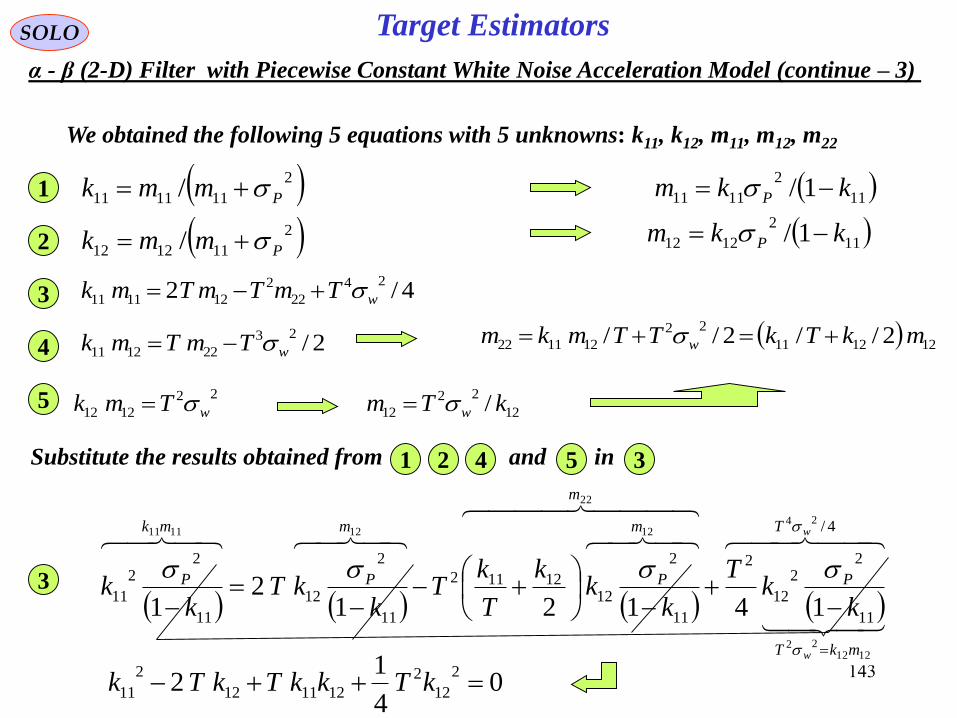
143
SOLO
11
2
1111 1/ kkm P
12
22
12 / kTm w
121211
22
121122 2//2// mkTkTTmkm w
We obtained the following 5 equations with 5 unknowns: k11, k12, m11, m12, m22
11
2
1212 1/ kkm P
2
111111 / Pmmk 1
2
111212 / Pmmk 2
4/224
22
2
121111 wTmTmTmk 3
2/23
221211 wTmTmk 4
22
1212 wTmk 5
Substitute the results obtained from and in1 2 34 5
4/
11
22
12
2
11
2
1212112
11
2
12
11
22
11
24
121222
22
12121111
141212
1
w
w
T
mkT
P
m
m
P
m
P
mk
P
kk
T
kk
k
T
kT
kkT
kk
3
04
12
2
12
2
121112
2
11 kTkkTkTk
α - β (2-D) Filter with Piecewise Constant White Noise Acceleration Model (continue – 3)
Target Estimators

144
SOLO
We obtained: 04
12
2
12
2
121112
2
11 kTkkTkTk
Kalata introduced the α, β parameters defined as: Tkk 1211 ::
and the previous equation is written as function of α, β as:
04
12 22
which can be used to write α as a function of β:2
2
12
22
11
2
1212
1 k
T
k
km wP
We obtained:
T
TTm wP
222
121
2
2
242
:1
P
wT
P
wT
2
: Target Maneuvering Index proportional to the ratio of:
Motion Uncertainty:
2
22Tw
Observation Uncertainty:2
P
α - β (2-D) Filter with Piecewise Constant White Noise Acceleration Model (continue – 4)
Target Estimators
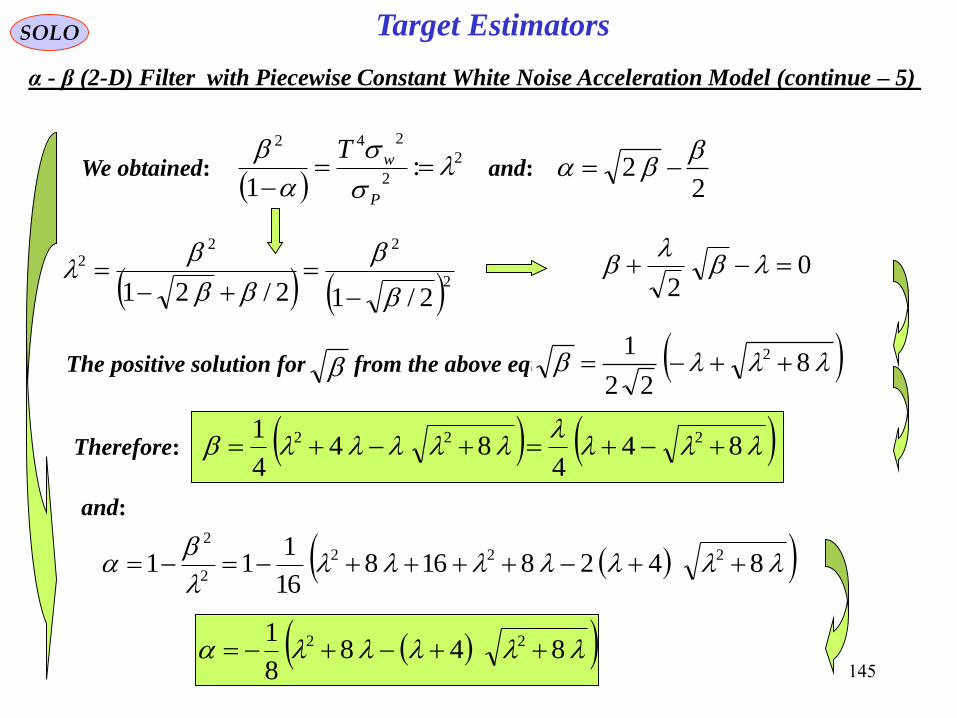
145
SOLO
22
We obtained:
2
2
242
:1
P
wT
02
The positive solution for from the above equation is: 822
1 2
Therefore:
844
844
1 222
and:
8428168
16
111 222
2
2
8488
1 22
and:
222
2
2/12/21
α - β (2-D) Filter with Piecewise Constant White Noise Acceleration Model (continue – 5)
Target Estimators

146
SOLO
We found
1212221211
12111111
2212
1211
1
11
mkmmk
mkmk
pp
pp
11
2
1111 1/ kkm P
11
2
1212 1/ kkm P
121211
22
121122
2//
2//
mkTk
TTmkm w
2
11111111 1 Pkmkp
2
12121112 1 Pkmkp
12
2//
2//
2
121211
121212121122
PT
TT
mkTk
mkmkTkp
2
11 Pp
2
12 PT
p
2
2221
2/P
Tp
&
α - β (2-D) Filter with Piecewise Constant White Noise Acceleration Model (continue – 6)
Target Estimators

147
8488
1 22
SOLO
We found
844
844
1 222
α, β gains, as function of λ in semi-log and log-log scales
α - β (2-D) Filter with Piecewise Constant White Noise Acceleration Model (continue – 7)
Target Estimators

148
SOLO
T
Tq
TT
TT
mm
mmT
pp
pp
Q
1
01
2/
2/3/
10
1
2
23
2212
1211
2212
1211
1
For White Noise acceleration model
qTmqTmTm
qTmTmqTmTmTm
mkmmk
mkmk
22
2
2212
2
2212
3
22
2
1211
1212221211
12111111
2/
2/3/2
1
11
qTmk
qTmTmk
qTmTmTmk
1212
2
221211
3
22
2
121111
2/
3/2
α - β (2-D) Filter with White Noise Acceleration Model
TT
TTqkQ
2/
2/3/
2
23
Target Estimators

149
SOLO
11
2
1111 1/ kkm P
1212 / kqTm
121211121122 2//2// mkTkqTTmkm
We obtained the following 5 equations with 5 unknowns: k11, k12, m11, m12, m22
11
2
1212 1/ kkm P
2
111111 / Pmmk 1
2
111212 / Pmmk 2
3/2 3
22
2
121111 qTmTmTmk 3
2/2
221211 qTmTmk 4
qTmk 12125
Substitute the results obtained from and in1 2 34 5
3/
11
22
12
2
11
2
1212112
11
2
12
11
22
11
3
1212
22
12121111
131212
1
qT
mkqT
P
m
m
P
m
P
mk
P
kk
T
kk
k
T
kT
kkT
kk
3
06
12
2
12
2
121112
2
11 kTkkTkTk
α - β (2-D) Filter with White Noise Acceleration Model (continue – 1)
Target Estimators

150
SOLO
We obtained: 06
12
2
12
2
121112
2
11 kTkkTkTk
The α, β parameters defined as: Tkk 1211 ::
and the previous equation is written as function of α, β as:
06
12 22
which can be used to write α as a function of β:212
22
1
/
1/ 11
2
12
12
12
T
k
k
T
qT
k
qTm P
We obtained:
2
2
32
:1
c
P
qT
α - β (2-D) Filter with White Noise Acceleration Model (continue – 2)
2
2
22
:
122
21
1c
The equation for solving β is:
which can be solved numerically.
Target Estimators

151
SOLO
We found
1212221211
12111111
2212
1211
1
11
mkmmk
mkmk
pp
pp
11
2
1111 1/ kkm P
11
2
1212 1/ kkm P
12121122 2// mkTkm
2
11111111 1 Pkmkp
2
12121112 1 Pkmkp
12
2//
2//
2
121211
121212121122
PT
TT
mkTk
mkmkTkp
2
11 Pp
2
12 PT
p
2
2221
2/P
Tp
&
α - β Filter with White Noise Acceleration Model (continue – 3)
Target Estimators

152
w
x
x
x
x
x
x
td
d
BA
1
0
0
000
100
010
SOLO
We want to find the steady-state form of the filter for
Assume that only the position measurements are available
kjjkkk
k
kkkk RvvEvEv
x
x
x
vxHz
1111
1
1111 0&001
Discrete System
1111
1
kkkk
kkkkk
vxHz
wxx
kjP
T
jkkkk
H
k
kjw
T
jkkkkk
vvERvxz
wwEQwT
T
xT
TT
x
k
kk
2
111111
2
22
1
&001
&
1
2/
100
10
2/1
1
α – β - γ (3-D) Filter with Piecewise Constant Wiener Process Acceleration Model
x
x
x
- position
- velocity
- acceleration
Target Estimators

153
SOLO
Piecewise (between samples) Constant White Noise acceleration model
12/
1
2/2
2
00 TTT
T
qlqkllwkwEk kl
TTT
12/
2/
2/2/2/
2
23
234
0
TT
TTT
TTT
qllwkwEk TT
Guideline for Choice of Process Noise Intensity
For this model q should be of the order of maximum acceleration increment over a
sampling period ΔaM.
A practical range is 0.5 ΔaM ≤ q ≤ ΔaM.
α – β - γ (3-D) Filter with Piecewise Constant Wiener Process Acceleration Model
(continue – 1)
Target Estimators
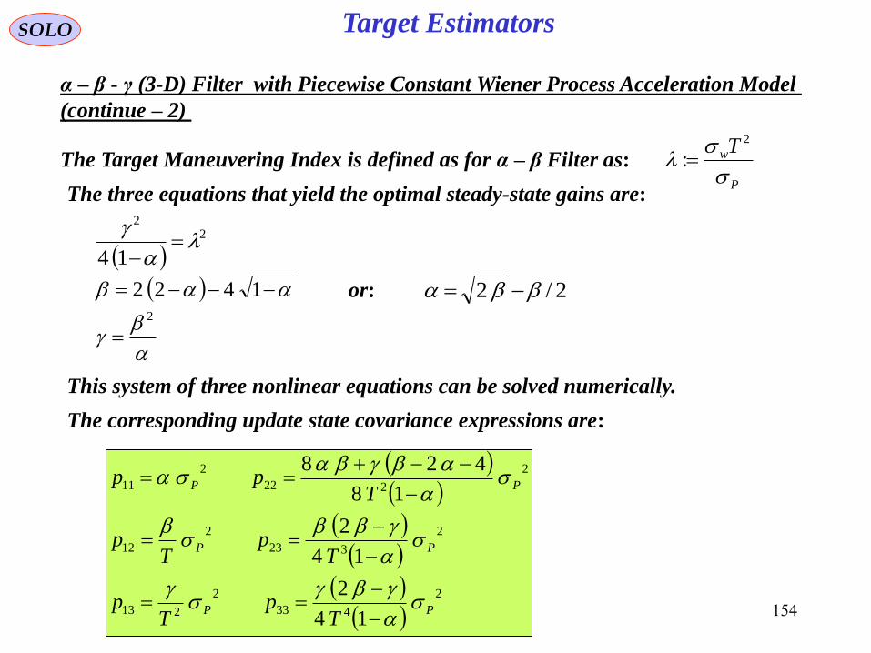
154
SOLO
The Target Maneuvering Index is defined as for α – β Filter as:P
wT
2
:
α – β - γ (3-D) Filter with Piecewise Constant Wiener Process Acceleration Model
(continue – 2)
The three equations that yield the optimal steady-state gains are:
2
2
14
1422 or: 2/2
2
This system of three nonlinear equations can be solved numerically.
The corresponding update state covariance expressions are:
2
433
2
213
2
323
2
12
2
222
2
11
14
2
14
2
18
428
PP
PP
PP
Tp
Tp
Tp
Tp
Tpp
Target Estimators

155
SOLOTarget Estimators
α – β - γ Filter gains as functions of λ in semi-log and log-log scales:
α – β - γ (3-D) Filter with Piecewise Constant Wiener Process Acceleration Model
(continue – 3)

156
SOLOTarget Estimators
α – β (2-D) Filter and α – β - γ (3-D) Filter - Summary
Advantages
Disadvantages
• Computation requirements (memory, computation time) are low.
• Quick (but possible dirty) evaluation of track performances as measured by the
steady-state variances.
• very limited capability in clutter.
• when used independently for each coordinate, one can encounter instabilities
due to decoupling.

157
SOLO Nonlinear Estimation (Filtering)
Return to Table of Content
Sensor Data
Processing and
Measurement
Formation
Observation -
to - Track
Association
Input
DataTrack
Maintenance
) Initialization,
Confirmation
and Deletion(
Filtering and
Prediction
Gating
Computations
Samuel S . Blackman , " Multiple-Target Tracking with Radar Applications ", Artech House ,
1986Samuel S . Blackman , Robert Popoli , " Design and Analysis of Modern Tracking Systems
", Artech House , 1999
The assumption of Linearity of the System and the Measurements
and the Gaussian assumption are not valid like:
• Angles , Range measurements (Measurements to states nonlinearities)
• Tracking in the presence of constraints
• Terrain Navigation
• Tracking Extended (non-point target)
Therefore we must deal with Nonlinear Filters and Use Approximations.

158
SOLO Nonlinear Estimation (Filtering)
Return to Table of Content
Sensor Data
Processing and
Measurement
Formation
Observation -
to - Track
Association
Input
DataTrack
Maintenance
) Initialization,
Confirmation
and Deletion(
Filtering and
Prediction
Gating
Computations
Samuel S . Blackman , " Multiple-Target Tracking with Radar Applications ", Artech House ,
1986Samuel S . Blackman , Robert Popoli , " Design and Analysis of Modern Tracking Systems
", Artech House , 1999
The Nonlinear Filters are approximations of the
Optimal Bayesian Estimators:
• Analytic Approximations (Linearization of the models)
- Extended Kalman Filter
• Sampling Approaches
- Unscented Kalman Filter, Particle Filter
• Numerical Integration
- Approximate p (xk|Z1:k) on a grid of nodes
• Gaussian Sum Filter
- Approximate p (xk|Z1:k) with a Gaussian Mixture

159
SOLO
Additive Gaussian Nonlinear Filter
kkk
kkk
vxhz
wxfx
11
Recursive Bayesian Estimation
k
xx
kkkkkkkkkkk xdPxxxhZxzEz 1|1|1:111| ,ˆ;,|ˆ N
T
kkkkkkkkkkkk
T
k
zz
kk zzRxdPxxxhxhP 1|1|1|1|1|ˆˆ,ˆ; N
T
kkkkkkkkkkk
T
k
xz
kk zxxdPxxxhxP 1|1|1|1|1|ˆˆ,ˆ; N
11|11|1111:11| .ˆ;|ˆk
xx
kkkkkkkkkk xdPxxxfZxEx N
T
kkkkkk
xx
kkkkkk
T
k
xx
kk xxQxdPxxxfxfP 1|1|111|11|11111|ˆˆ,ˆ; N
Summary (see “Bayesian Estimation” presentation)
The Kalman Filter, that uses this computations is given by:
1|
1
1|1|1||ˆˆ|ˆ
kkk
K
zz
kk
xz
kkkkkkkk zzPPxzxEx
k
T
k
zz
kkk
xx
kk
zx
kk
zz
kk
xx
kk
xx
kkk
T
kkkkkk
xx
kk
KPKP
PPPPZxxxxEP
1
1|1|
1|
1
1|1|1|:1|||ˆˆ
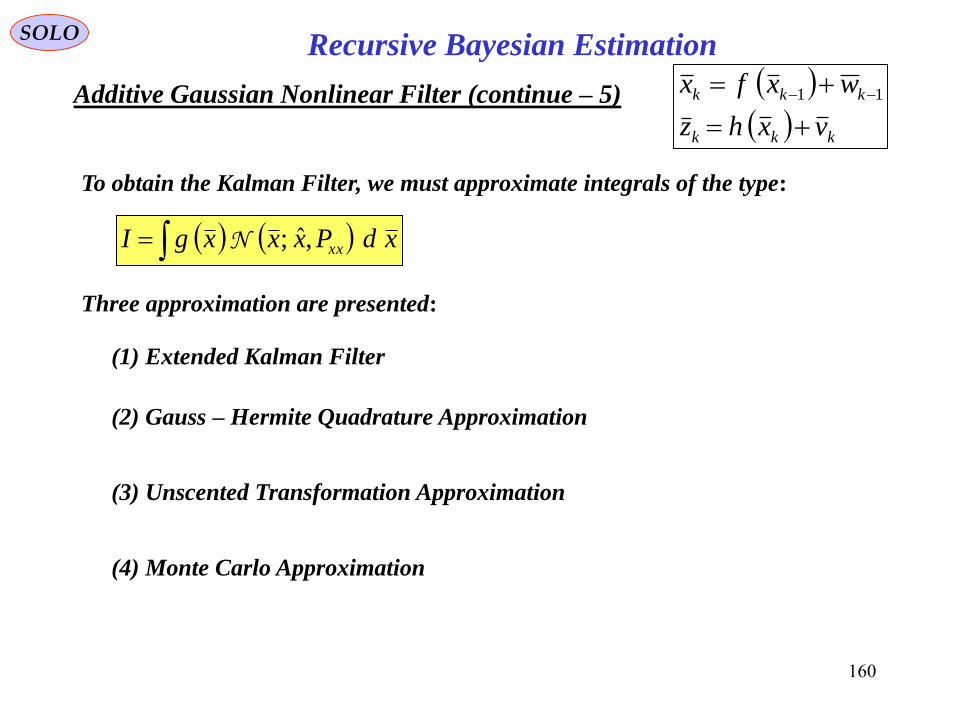
160
SOLO
Additive Gaussian Nonlinear Filter (continue – 5)
kkk
kkk
vxhz
wxfx
11
Recursive Bayesian Estimation
xdPxxxgI xx,ˆ;N
To obtain the Kalman Filter, we must approximate integrals of the type:
Three approximation are presented:
(2) Gauss – Hermite Quadrature Approximation
(3) Unscented Transformation Approximation
(4) Monte Carlo Approximation
(1) Extended Kalman Filter

161
Extended Kalman FilterSensor Data
Processing and
Measurement
Formation
Observation -
to - Track
Association
Input
Data Track Maintenance
( Initialization,
Confirmation
and Deletion)
Filtering and
Prediction
Gating
Computations
Samuel S. Blackman, " Multiple-Target Tracking with Radar Applications", Artech House,
1986Samuel S. Blackman, Robert Popoli, " Design and Analysis of Modern Tracking Systems",
Artech House, 1999
SOLO
In the extended Kalman filter, (EKF) the state transition
and observation models need not be linear functions of
the state but may instead be (differentiable) functions.
11,1,1 kwkukxkfkx
kkukxkhkz ,,
State vector dynamics
Measurements
kPkekeEkxEkxke x
T
xxx &:
lk
T
www kQlekeEkwEkwke ,
0
&:
lklekeET
vw ,0
lk
lklk
1
0,
The function f can be used to compute the predicted state from the previous estimate
and similarly the function h can be used to compute the predicted measurement from
the predicted state. However, f and h cannot be applied to the covariance directly.
Instead a matrix of partial derivatives (the Jacobian) is computed.
1112
1111,1,11,1,1
1
2
2
1
kekex
fkeke
x
fkekukxEkfkukxkfke wx
Hessian
kxE
T
xx
Jacobian
kxE
wx
kkex
hkeke
x
hkkukxEkhkukxkhke x
Hessian
kxE
T
xx
Jacobian
kxE
z
2
2
12
1,,,,
Taylor’s Expansion:
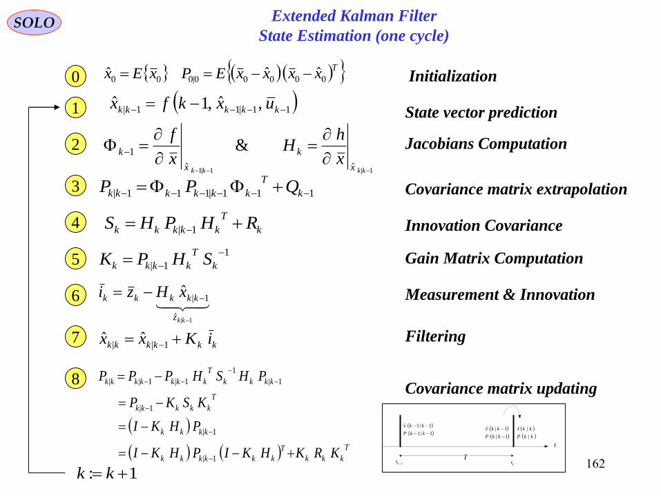
162
Extended Kalman Filter
State Estimation (one cycle)SOLO
1|1
1|1ˆ
kkP
kkx
1kt ktT
t
1|
1|ˆ
kkP
kkx kkP
kkx
|
|ˆ
1: kk
11|11| ,ˆ,1ˆ kkkkk uxkfx
State vector prediction1
Jacobians Computation
1|1|1 ˆˆ
1 &
kkkk x
k
x
kx
hH
x
f2
Covariance matrix extrapolation111|111| k
T
kkkkkk QPP3
Innovation Covariancek
T
kkkkk RHPHS 1|4
Gain Matrix Computation1
1|
k
T
kkkk SHPK5
Measurement & Innovation1|ˆ
1|ˆ
kkz
kkkkk xHzi6
Filteringkkkkkk iKxx 1||
ˆˆ7
Covariance matrix updating
T
kkk
T
kkkkkk
kkkk
T
kkkkk
kkkk
T
kkkkkkk
KRKHKIPHKI
PHKI
KSKP
PHSHPPP
1|
1|
1|
1|
1
1|1||8
0 Initialization TxxxxEPxEx 00000|000ˆˆˆ

163
Extended Kalman Filter
State Estimation (one cycle)
Sensor Data
Processing and
Measurement
Formation
Observation -
to - Track
Association
Input
Data Track Maintenance
( Initialization,
Confirmation
and Deletion)
Filtering and
Prediction
Gating
Computations
Samuel S. Blackman, " Multiple-Target Tracking with Radar Applications", Artech House,
1986Samuel S. Blackman, Robert Popoli, " Design and Analysis of Modern Tracking Systems",
Artech House, 1999
SOLO
Evolution
of the system
(true state)
Estimation
of the state
State Covariance and
Kalman Filter ComputationsController
Innovation Covariance
k
T
kkkkk RHPHS 1|
Innovation
1|ˆ
kkkk zz
1kt
kt
Time
Jacobians Evaluation
kk
kk
xx
k
xx
k
x
hH
x
f
|
1|1
ˆ
ˆ
1
State at tk-1
1kxControl at tk-1
1ku
State
Estimation
at tk-1
1|1ˆ
kkx
State Error Covariance
at tk-1 1|1 kkP
State Prediction Covariance
111|111| k
T
kkkkkk QPP
State Prediction
at tk 11|11| ,ˆ,1ˆ
kkkkk uxkfx
Measurement Prediction
at tk 1|1|
ˆ,ˆ kkkk xkhz
Transition to tk
111,,1 kkkk wuxkfx
Measurement at tk
kkk vxkhz ,
Kalman Filter Gain
1
1|
k
T
kkkk SHPK
Update State
Covariance at tkk k
T
kkkkkkk KSKPP 1||
Update State
Estimation at t k
kkkkkk Kxx 1||ˆˆ
I.C.: 00|0ˆ xEx T
xxxxEP 0|000|000|0ˆˆ I.C.:
1|1ˆ
kkx
1kx
kkP |
2|1 kkP
kkx |ˆ
kx
1|1 kkP
1| kkP
1|ˆ
kkx
1kt kt
Real Trajectory
Estimated
Trajectory
Rudolf E. Kalman
( 1920 - )

164
Extended Kalman FilterSOLO
Criticism of the Extended Kalman FilterUnlike its linear counterpart, the extended Kalman filter is not an optimal estimator.
In addition, if the initial estimate of the state is wrong, or if the process is modeled
incorrectly, the filter may quickly diverge, owing to its linearization. Another problem
with the extended Kalman filter is that the estimated covariance matrix tends to
underestimate the true covariance matrix and therefore risks becoming inconsistent
in the statistical sense without the addition of "stabilizing noise".
Having stated this, the Extended Kalman filter can give reasonable performance, and
is arguably the de facto standard in navigation systems and GPS.

165
SOLO
Additive Gaussian Nonlinear Filter (continue – 5)
kkk
kkk
vxhz
wxfx
11
Recursive Bayesian Estimation
xdPxxxgI xx,ˆ;N
To obtain the Kalman Filter, we must approximate integrals of the type:
Gauss – Hermite Quadrature Approximation
xdxxPxxP
xgI xx
T
xx
nˆˆ
2
1exp
2
1 1
2/1
Let Pxx = STS a Cholesky decomposition, and define: xxSz ˆ2
1: 1
zdezgI zz
n
T
2/2
2
This integral can be approximated using the Gauss – Hermite
quadrature rule:
M
i
ii
z zfwzdzfe1
2
Carl Friedrich
Gauss
1777 - 1855
Charles Hermite
1822 - 1901
Andre – Louis
Cholesky
1875 - 1918

166
SOLO
Additive Gaussian Nonlinear Filter (continue – 6)
kkk
kkk
vxhz
wxfx
11
Recursive Bayesian Estimation
Gauss – Hermite Quadrature Approximation (continue – 1)
M
i
ii
z zfwzdzfe1
2
The quadrature points zi and weights wi are defined as follows:
A set of orthonormal Hermite polynomials are generated from the recurrence relationship:
zHj
jzH
jzzH
zHzH
jjj 11
4/1
01
11
2
/1,0
or in matrix form:
Mjj
zH
zH
zH
zH
zH
zH
zH
z jM
e
M
zh
M
J
M
M
zh
M
M
M
,,2,12
:
1
0
0
0
00
00
00
00
00
1
1
0
1
1
2
21
1
1
1
0
zHj
zHj
zHz jjj
jj
11
1
2
1
2
zHezhJzhz MMMM
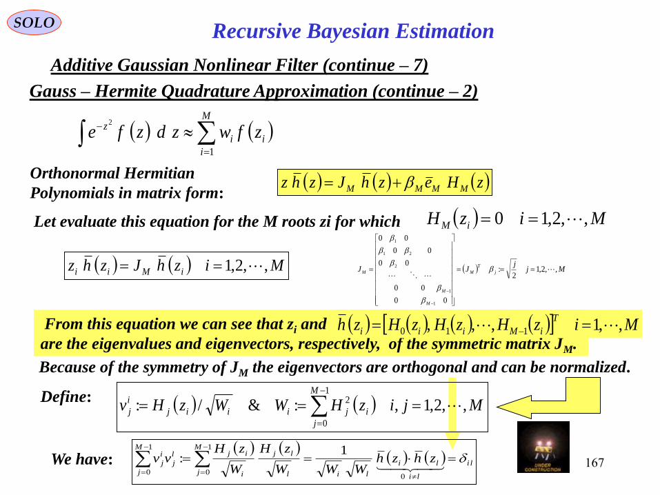
167
SOLO
Additive Gaussian Nonlinear Filter (continue – 7)
Recursive Bayesian Estimation
Gauss – Hermite Quadrature Approximation (continue – 2)
M
i
ii
z zfwzdzfe1
2
Orthonormal Hermitian
Polynomials in matrix form:
Mjj
JJ j
T
M
M
M
M ,,2,12
:
00
00
00
00
00
1
1
2
21
1
zHezhJzhz MMMM
Let evaluate this equation for the M roots zi for which MizH iM ,,2,10
MizhJzhz iMii ,,2,1
From this equation we can see that zi and
are the eigenvalues and eigenvectors, respectively, of the symmetric matrix JM.
MizHzHzHzhT
iMiii ,,1,,, 110
Because of the symmetry of JM the eigenvectors are orthogonal and can be normalized.
Define: MjizHWWzHvM
j
ijiiij
i
j ,,2,1,:&/:1
0
2
We have:
li
li
li
li
M
j l
lj
i
ijM
j
l
j
i
j zhzhWWW
zH
W
zHvv
0
1
0
1
0
1:

168
Uscented Kalman FilterSOLO
When the state transition and observation models – that is, the predict and update
functions f and h (see above) – are highly non-linear, the Extended Kalman Filter
can give particularly poor performance [JU97]. This is because only the mean is
propagated through the non-linearity. The Unscented Kalman Filter (UKF) [JU97]
uses a deterministic sampling technique known as the to pick a minimal set of
sample points (called “sigma points”) around the mean. These “sigma points” are
then propagated through the non-linear functions and the covariance of the estimate
is then recovered. The result is a filter which more accurately captures the true mean
and covariance. (This can be verified using Monte Carlo sampling or through a
Taylor series expansion of the posterior statistics.) In addition, this technique
removes the requirement to analytically calculate Jacobians, which for complex
functions can be a difficult task in itself.
111,,1 kkkk wuxkfx
kkk xkhz ,
State vector dynamics
Measurements
kPkekeEkxEkxke x
T
xxx &:
lk
T
www kQlekeEkwEkwke ,
0
&:
lklekeET
vw ,0
lk
lklk
1
0,
The Unscented Algorithm using kPkekeEkxEkxke x
T
xxx &:
determines kPkekeEkzEkzke z
T
zzz &:

169
Unscented Kalman FilterSOLO
n
n
j j
j
n
x
n
x
n
x
x
xxx
fxn
xxf
1
0
ˆ
:
!
1ˆ
Develop the nonlinear function f in a Taylor series around x
Define also the operator xfx
xfxfD
nn
j j
jx
n
x
n
x
x
1
:
Propagating Means and Covariances Through Nonlinear Transformations
Consider a nonlinear function . xfy
Let compute
Assume is a random variable with a probability density function pX (x) (known or
unknown) with mean and covariance
x Txx xxxxEPxEx ˆˆ,ˆ
0ˆ
10
ˆ
0
!
1
!
1
!
1ˆˆ
nx
nn
j j
j
n
x
n
x
n
n
x
fx
xEn
fxEn
DEn
xxfEy
x
xxTT PxxxxExxE
xxExE
xxx
ˆˆ
0ˆ
ˆ

170
Unscented Kalman FilterSOLO
Propagating Means and Covariances Through Nonlinear Transformations
Consider a nonlinear function .
(continue – 1)
xfy
xxTT PxxxxExxE
xxExE
xxx
ˆˆ
0ˆ
ˆ
x
n
j j
jx
n
j j
jx
n
j j
j
x
n
j j
j
n
x
nn
j j
j
fx
xEfx
xEfx
xE
fx
xExffx
xEn
xxfEy
xxx
xx
ˆ
4
1
ˆ
3
1
ˆ
2
1
ˆ
10
ˆ
1
!4
1
!3
1
!2
1
ˆ!
1ˆˆ
Since all the differentials of f are computed around the mean (non-random) x
xx
xxT
xxx
TT
xxx
TT
xxx fPfxxEfxxEfxEˆˆˆˆ
2
0
ˆ1
0ˆ1
ˆ0
ˆ
x
n
j j
j
x
n
j j
j
x
xxx fx
xEfx
xEfxEfxExx
xxxxxx
xxT
x
n
x
n
x fDEfDEfPxffDEn
xxfEy ˆ
4
ˆ
3
ˆ
0
ˆ!4
1
!3
1
!2
1ˆ
!
1ˆˆ

171
Simon J. Julier
Unscented Kalman FilterSOLO
Propagating Means and Covariances Through Nonlinear Transformations
Consider a nonlinear function .
(continue - 2)
xfy
xxTT PxxxxExxE
xxExE
xxx
ˆˆ
0ˆ
ˆ
Unscented Transformation (UT), proposed by Julier and Uhlmann
uses a set of “sigma points” to provide an approximation of
the probabilistic properties through the nonlinear function
Jeffrey K. Uhlman
A set of “sigma points” S consists of p+1 vectors and their associated
weights S = { i=0,1,..,p: x(i) , W(i) }.
(1) Compute the transformation of the “sigma points” through the
nonlinear transformation f:
pixfy ii ,,1,0
(2) Compute the approximation of the mean:
p
i
ii yWy0
ˆ
The estimation is unbiased if:
yWyyEWyWEp
i
ip
iy
iip
i
ii ˆˆ00
ˆ0
1
0
p
i
iW
(3) The approximation of output covariance is given by
p
i
Tiiiyy yyyyWP0
ˆˆ

172
Unscented Kalman FilterSOLO
Propagating Means and Covariances Through Nonlinear Transformations
Consider a nonlinear function (continue – 3) xfy
One set of points that satisfies the above conditions consists of a symmetric set of symmetric
p = 2nx points that lie on the covariance contour Pxx:th
xn
x
x
ni
x
i
xxxni
i
xxxi
ni
nWW
nWW
PW
nxx
PW
nxx
WWxx
x
x ,,1
2/1
2/1
1ˆ
1ˆ
ˆ
0
0
0
0
0
00
where is the row or column of the matrix square root of nx Pxx /(1-W0)
(the original covariance matrix Pxx multiplied by the number of dimensions of x, nx/(1-W0)).
This implies:
i
xx
x WPn 01/
xxx
n
i
T
i
xxx
i
xxx PW
nP
W
nP
W
nx
01 00 111
Unscented Transformation (UT) (continue – 1)

173
Unscented Kalman FilterSOLO
Propagating Means and Covariances Through Nonlinear Transformations
Consider a nonlinear function (continue – 3) xfy
Unscented Transformation (UT) (continue – 2)
0
0
2,,1ˆ!
1
,,1ˆ!
1
0ˆ
n
xx
n
x
n
x
n
x
ii
nnixfDn
nixfDn
ixf
xfy
i
i
1
Unscented Algorithm:
x
ii
x
i
x
iii
x
i
x
i
x
n
i
xx
x
n
i
x
x
n
i
xxx
x
n
i n
n
x
x
n
i n
n
x
x
n
i
ii
UT
xfDxfDn
WxfD
n
Wxf
xfDxfDxfDxfn
WxfW
xfDnn
WxfD
nn
WxfWyWy
1
640
1
20
1
64200
1 0
0
1 0
00
2
0
ˆ!6
1ˆ
!4
11ˆ
2
11ˆ
ˆ!6
1ˆ
!4
1ˆ
!2
1ˆ
1ˆ
ˆ!
1
2
1ˆ
!
1
2
1ˆˆ
i
xxxi
i PW
nxxxx
01ˆˆ
2 Since
oddnxfD
evennxfDxf
xxxfD
n
x
n
x
nn
j j
ij
n
x
i
ix
i
ˆ
ˆˆˆ
1

174
Unscented Kalman Filter
x
ii
n
i
xx
x
xxT
UT xfDxfDn
WxfPxfy
1
640 ˆ!6
1ˆ
!4
11ˆ
2
1ˆˆ
i
xxxi
i PW
nxxxx
01ˆˆ
SOLO
Propagating Means and Covariances Through Nonlinear Transformations
Consider a nonlinear function (continue – 4) xfy
Unscented Transformation (UT) (continue – 3)
Unscented Algorithm:
xfPxfPW
n
n
WxfP
W
nP
W
n
n
W
xfPW
nP
W
n
n
WxfD
n
W
xxTxxxT
x
n
i
T
i
xxx
i
xxxT
x
n
i
T
i
xxx
i
xxxT
x
n
i
x
x
x
xx
i
ˆ2
1ˆ
12
11ˆ
112
11
ˆ112
11ˆ
2
11
0
0
1 00
0
1 00
0
1
20
Finally:
We found
xxxxxx
xxT
x
n
x
n
x fDEfDEfPxffDEn
xxfEy ˆ
4
ˆ
3
ˆ
0
ˆ!4
1
!3
1
!2
1ˆ
!
1ˆˆ
We can see that the two expressions agree exactly to the third order.

175
covariance
mean
Actual (sampling)
xfy
true mean
true
covariance
covariance
mean
Actual (sampling) Linearized (EKF)
xfy
APAP
xfy
xxTyy
ˆˆ
true mean
true
covariance
xf ˆAPA xxT
Uscented Kalman FilterSOLO
covariance
mean
sigma points
Actual (sampling) Linearized (EKF)Unscented
Transformation
xfy
APAP
xfy
xxTyy
ˆˆ XY f
transformed
sigma points
UT mean
UT covariance
true mean
true
covariance
xf ˆAPA xxT
weighted sample mean
and covariance
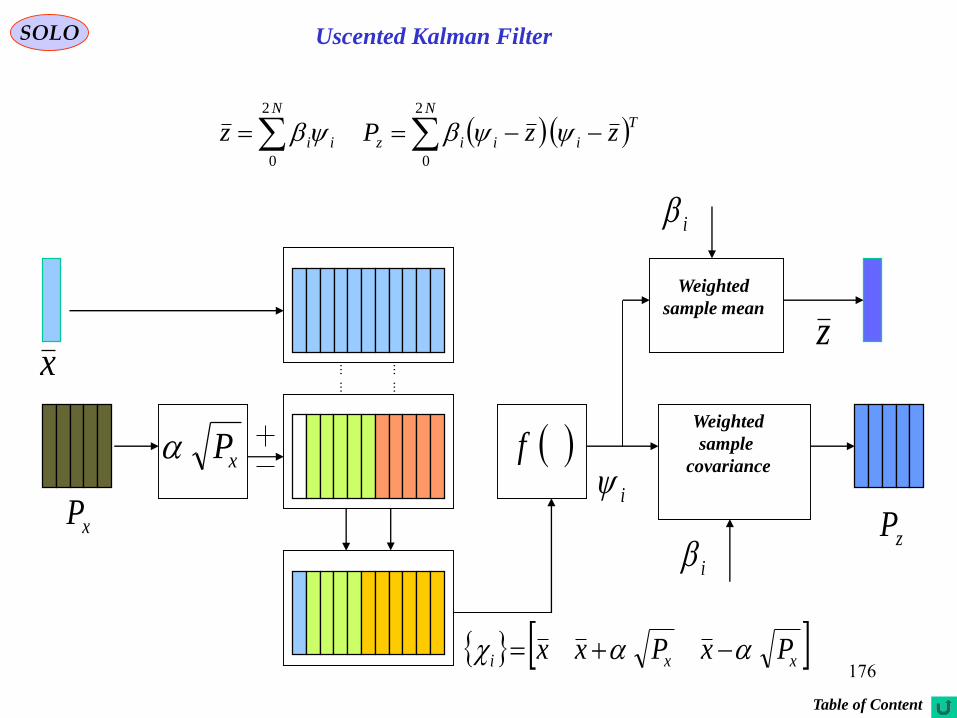
176
Uscented Kalman FilterSOLO
N
T
iiiz
N
ii zzPz2
0
2
0
x
xP
xP
zP
f
i
i
i
z
xxi PxPxx
Weighted
sample mean
Weighted
sample
covariance
Table of Content

177
Uscented Kalman FilterSOLO
UKF Summary
Initialization of UKF
TxxxxEPxEx 00000|000ˆˆˆ
R
Q
P
xxxxEPxxExTaaaaaTTaa
00
00
00
ˆˆ00ˆˆ
0|0
00000|0000
TTTTa vwxx :
For ,,1k
System Definition
lkk
T
lkkkkk
lkk
T
lkkkkkk
RvvEvEvxkhz
QwwEwEwuxkfx
,
,1111111
&0,
&0,,1
Liuxkfx k
i
kk
i
kk 2,,1,0,ˆ,1ˆ11|11|
Li
LW
LWxWx m
i
mL
i
i
kk
m
ikk 2,,12
1&ˆˆ
0
2
0
1|1|
0
Calculate the Sigma Points
L
LiPxx
LiPxx
xx
i
kkkk
Li
kk
i
kkkk
i
kk
kkkk
,,1ˆˆ
,,1ˆˆ
ˆˆ
1|11|11|1
1|11|11|1
1|1
0
1|1
1
State Prediction and its Covariance2
Li
LW
LWxxxxWP c
i
cL
i
T
kk
i
kkkk
i
kk
c
ikk 2,,12
1&1ˆˆˆˆ 2
0
2
0
1|1|1|1|1|
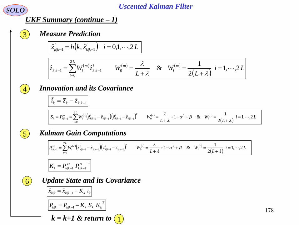
178
Uscented Kalman FilterSOLO
UKF Summary (continue – 1)
Lixkhz i
kk
i
kk 2,,1,0ˆ,ˆ1|1|
Li
LW
LWzWz m
i
mL
i
i
kk
m
ikk 2,,12
1&ˆˆ
0
2
0
1|1|
Measure Prediction3
Innovation and its Covariance4
1|ˆ
kkkk zzi
Li
LW
LWzzzzWPS c
i
cL
i
T
kk
i
kkkk
i
kk
c
i
zz
kkk 2,,12
1&1ˆˆˆˆ 2
0
2
0
1|1|1|1|1|
Kalman Gain Computations5
Li
LW
LWzzxxWP c
i
cL
i
T
kk
i
kkkk
i
kk
c
i
xz
kk 2,,12
1&1ˆˆˆˆ 2
0
2
0
1|1|1|1|1|
1
1|1|
zz
kk
xz
kkk PPK
Update State and its Covariance6
kkkkkk iKxx 1||ˆˆ
T
kkkkkkk KSKPP 1||
k = k+1 & return to 1

179
Unscented Kalman Filter
State Estimation (one cycle)
Sensor Data
Processing and
Measurement
Formation
Observation -
to - Track
Association
Input
Data Track Maintenance
( Initialization,
Confirmation
and Deletion)
Filtering and
Prediction
Gating
Computations
Samuel S. Blackman, " Multiple-Target Tracking with Radar Applications", Artech House,
1986Samuel S. Blackman, Robert Popoli, " Design and Analysis of Modern Tracking Systems",
Artech House, 1999
SOLO
Evolution
of the system
(true state)
Estimation
of the state
State Covariance and
Kalman Filter ComputationsController
Innovation
1|ˆ
kkkk zz
1kt
kt
Time
State at tk-1
1kxControl at tk-1
1ku
State
Estimation
at tk-1
1|1ˆ
kkx
State Error Covariance
at tk-1 1|1 kkP
State Prediction Covariance
L
i
T
kk
i
kkkk
i
kk
c
ikk xxxxWP2
0
1|1|1|1|1|ˆˆˆˆ
Li
uxkfx k
i
kk
i
kk
2,,1,0
,ˆ,1ˆ11|11|
Li
xkhz i
kk
i
kk
2,,1,0
ˆ,ˆ1|1|
Transition to tk
111,,1 kkkk wuxkfx
Measurement at tk
kkk vxkhz ,
Update State
Covariance at tkk k
T
kkkkkkk KSKPP 1||
Update State
Estimation at t k
kkkkkk Kxx 1||ˆˆ
State Prediction at tk
L
i
i
kk
m
ikk xWx2
0
1|1|ˆˆ
Sigma Points Computation
LiPxx
LiPxx
xx
i
kkkk
Li
kk
i
kkkk
i
kk
kkkk
,,1ˆˆ
,,1ˆˆ
ˆˆ
1|11|11|1
1|11|11|1
1|1
0
1|1
Measurement Prediction at tk
L
i
i
kk
m
ikk zWz2
0
1|1|ˆˆ
Innovation Covariance
L
i
T
kk
i
kkkk
i
kk
c
i
zz
kkk
zzzzW
PS
2
0
1|1|1|1|
1|
ˆˆˆˆ
1
||
zz
ykk
zx
ykkk PPK
L
i
T
kk
i
kkkk
i
kk
c
i
zz
kk zzxxWP2
0
1|1|1|1|1|ˆˆˆˆ
Kalman Filter Gain
I.C.: 00|0ˆ xEx T
xxxxEP 0|000|000|0ˆˆ I.C.:
1|1ˆ
kkx
1kx
kkP |
2|1 kkP
kkx |ˆ
kx
1|1 kkP
1| kkP
1|ˆ
kkx
1kt kt
Real Trajectory
Estimated
Trajectory
covariance
mean
sigma points
Actual (sampling) Unscented
Transformation
xfy
XY f
transformed
sigma points
UT mean
UT covariance
true mean
true
covariance
APA xxT
weighted sample mean
and covariance
Simon J. Julier Jeffrey K. Uhlman

180
Numerical Integration Using a Monte Carlo Approximation
sN
1
SOLO
A Monte Carlo Approximation of the Expected Value Integrals uses Discrete
Approximation to the Gaussian PDF xxPxx ,ˆ;N
xxPxx ,ˆ;N can be approximated by:
ss N
i
i
s
N
i
iixx xxN
xxwPxxx11
1,ˆ; Np
We can see that for any x we have
x
xx
xx
i
i
x N
i
ii dPxwdxw
i
s
,ˆ;1
N
The weight wi is not the probability of the point xi. The probability density near xi is
given by the density of the points in the region around xi, which can be obtained by a
normalized histogram of all xi.
Draw Ns samples from , where {xi , i = 1,2,…,Ns} are a set of support
points (random samples of particles) with weights {wi = 1/Ns, i=1,2,…,Ns}
xxPxx ,ˆ;N
Monte Carlo Kalman Filter (MCKF)
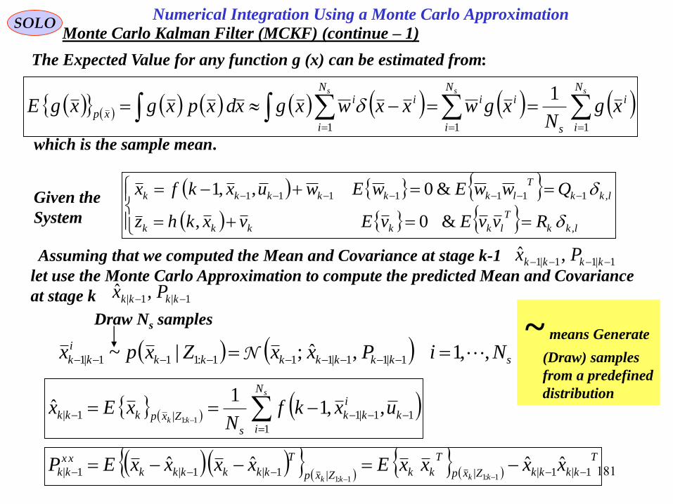
181
Numerical Integration Using a Monte Carlo ApproximationSOLO
The Expected Value for any function g (x) can be estimated from:
sss N
i
i
s
N
i
iiN
i
ii
xpxg
NxgwxxwxgxdxpxgxgE
111
1
which is the sample mean.
lkk
T
lkkkkk
lkk
T
lkkkkkk
RvvEvEvxkhz
QwwEwEwuxkfx
,
,1111111
&0,
&0,,1
Given the
System
Assuming that we computed the Mean and Covariance at stage k-1
let use the Monte Carlo Approximation to compute the predicted Mean and Covariance
at stage k
1|11|1 ,ˆ kkkk Px
1|1| ,ˆ kkkk Px
s
kk
N
i
k
i
kk
s
Zxpkkk uxkfN
xEx1
11|1|1| ,,11
ˆ1:1
T
kkkkZxp
T
kkZxp
T
kkkkkk
xx
kk xxxxExxxxEPkkkk
1|1|||1|1|1|ˆˆˆˆ
1:11:1
Monte Carlo Kalman Filter (MCKF) (continue – 1)
Draw Ns samples
skkkkkkk
i
kk NiPxxZxpx ,,1,ˆ;|~ 1|11|111:111|1 N~ means Generate
(Draw) samples
from a predefined
distribution
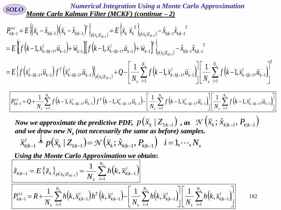
182
Numerical Integration Using a Monte Carlo ApproximationSOLO
T
N
i
k
i
kk
s
N
i
k
i
kk
sZxpk
i
kk
T
k
i
kk
T
kkkkZxp
T
kk
i
kkkk
i
kk
T
kkkkZxp
T
kkZxp
T
kkkkkk
xx
kk
ss
kk
kk
kkkk
uxkfN
uxkfN
QuxfuxfE
xxwuxkfwuxkfE
xxxxExxxxEP
1
11|1
1
11|1|11|111|1
1|1||111|1111|1
1|1|||1|1|1|
,,11
,,11
,,
ˆˆ,,1,,1
ˆˆˆˆ
1:1
1:1
1:11:1
sss N
i
k
i
kk
s
N
i
k
i
kk
s
N
i
k
i
kk
T
k
i
kk
s
xx
kk uxkfN
uxkfN
uxkfuxkfN
QP1
11|1
1
11|1
1
11|111|11| ,,11
,,11
,,1,,11
Using the Monte Carlo Approximation we obtain:
s
kk
N
i
i
kk
s
Zxpkkk xkhN
zEz1
1||1| ,1
ˆ1:1
sss N
i
i
kk
s
N
i
i
kk
s
N
i
i
kk
Ti
kk
s
zz
kk xkhN
xkhN
xkhxkhN
RP1
1|
1
1|
1
1|1|1| ,1
,1
,,1
Monte Carlo Kalman Filter (MCKF) (continue – 2)
skkkkkkk
i
kk NiPxxZxpx ,,1,ˆ;|~ 1|1|1:11| N
Now we approximate the predictive PDF, , as
and we draw new Ns (not necessarily the same as before) samples.
1:1| kk Zxp 1|1| ,ˆ; kkkkk PxxN

183
Numerical Integration Using a Monte Carlo ApproximationSOLO
In the same way we obtain:
sss N
i
i
kk
s
N
i
i
kk
s
N
i
i
kk
Ti
kk
s
zx
kk xkhN
xN
xkhxN
P1
1|
1
1|
1
1|1|1| ,11
,1
Monte Carlo Kalman Filter (MCKF) (continue – 3)
The Kalman Filter Equations are:
1
1|1|
zz
kk
zx
kkk PPK
1|1||ˆˆˆ
kkkkkkkk zzKxx
T
k
zz
kkk
xx
kk
xx
kk KPKPP 1|1||
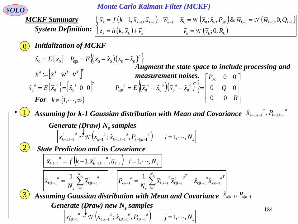
184
Monte Carlo Kalman Filter (MCKF)SOLO
MCKF Summary
TxxxxEPxEx 00000|000ˆˆˆ
R
Q
P
xxxxEPxxExTaaaaaTTaa
00
00
00
ˆˆ00ˆˆ
0|0
00000|0000
For ,,1k
System Definition:
kkkkkk
kkkkkkk
Rvvvxkhz
QwwPxxxwuxkfx
,0;,
,0;&,ˆ;,,1 1110|0000111
N
NN
sk
ai
kk
ai
kk Niuxkfx ,,1,,1 11|11|
sN
i
ai
kk
s
a
kk xN
x1
1|1|
1ˆ
Initialization of MCKF0
State Prediction and its Covariance2
Ta
kk
a
kk
N
i
Tai
kk
ai
kk
s
a
kk xxxxN
Ps
1|1|
1
1|1|1|ˆˆ
1
Assuming for k-1 Gaussian distribution with Mean and Covariance1a
kk
a
kk Px 1|11|1 ,ˆ
Assuming Gaussian distribution with Mean and Covariance3 1|1| ,ˆ kkkk Px
s
a
kk
a
kk
a
k
ai
kk NiPxxx ,,1,ˆ;~ 1|11|111|1 N
Generate (Draw) Ns samples
s
a
kk
a
kk
a
kk
aj
kk NjPxxx ,,1,ˆ;~ 1|1|1|1| N
Generate (Draw) new Ns samples
TTTTa vwxx :Augment the state space to include processing and
measurement noises.

185
Monte Carlo Kalman Filter (MCKF)SOLO
MCKF Summary (continue – 1)
s
aj
kk
j
kk Njxkhz ,,1, 1|1|
sN
j
j
kk
s
kk zN
z1
1|1|
1ˆ
Measure Prediction4
sN
j
T
kk
j
kkkk
j
kk
s
zz
kkk zzzzN
PS1
1|1|1|1|1|ˆˆ
1
Innovation and its Covariance 1|ˆ
kkkk zzi7
s
aN
j
T
kk
j
kk
a
kk
aj
kk
s
zx
kk zzxxN
P1
1|1|1|1|1|ˆˆ
1
6 Kalman Gain Computations1
1|1|
zz
kk
zx
kk
a
k PPKa
Kalman Filter8k
a
k
a
kk
a
kk iKxx 1||ˆˆ
Ta
kk
a
k
a
kk
a
kk KSKPP 1||
k := k+1 & return to 1
Predicted Covariances Computations5

186
Sensor Data
Processing and
Measurement
Formation
Observation -
to - Track
Association
Input
Data Track Maintenance
( Initialization,
Confirmation
and Deletion)
Filtering and
Prediction
Gating
Computations
Samuel S. Blackman, " Multiple-Target Tracking with Radar Applications", Artech House,
1986Samuel S. Blackman, Robert Popoli, " Design and Analysis of Modern Tracking Systems",
Artech House, 1999
SOLO
Evolution
of the system
(true state)
Estimation
of the state
State Covariance and
Kalman Filter ComputationsController
Innovation
1|ˆ
kkkk zz
1kt
kt
Time
State at tk-1
1kxControl at tk-1
1ku
State
Estimation
at tk-1
a
kkx 1|1ˆ
State Error Covariance
at tk-1 a
kkP 1|1
s
ai
kk
i
kk
Ni
xkhz
,,1
, 1|1|
Transition to tk
111,,1 kkkk wuxkfx
Measurement at tk
kkk vxkhz ,
Update State
Covariance at tkk kTa
kk
a
k
a
kk
a
kk KSKPP 1||
Update State
Estimation at t k
k
a
k
a
kk
a
kk Kxx 1||ˆˆ
State Prediction at tk
sN
i
k
ai
kk
s
a
kk uxkN
x1
11|11| ,,11
ˆ
Measurement Prediction at tk
sN
i
i
kk
s
kk zN
z0
1|1|
1ˆ
Innovation Covariance
sN
i
T
kk
i
kkkk
i
kk
s
zz
kkk
zzzzN
PS
1
1|1|1|1|
1|
ˆˆ1
1
1|1|
zz
kk
zx
kk
a
k PPKa
s
aN
i
T
kk
i
kk
a
kk
ai
kk
s
zx
kk zzxxN
P1
1|1|1|1|1|ˆˆ
1Kalman Filter Gain
I.C.: Taxx 0,0,ˆˆ
0|00|0 kk
aRQPdiagP ,, 10|00|0 I.C.:
1|1ˆ
kkx
1kx
kkP |
2|1 kkP
kkx |ˆ
kx
1|1 kkP
1| kkP
1|ˆ
kkx
1kt kt
Real Trajectory
Estimated
Trajectory
Generate Prior Samples
s
a
kk
a
kk
a
k
ai
kk
Ni
Pxxx
,,1
,ˆ;~ 1|11|111|1
N
Generate Predictive Samples
s
a
kk
a
kk
a
k
ai
kk
Ni
Pxxx
,,1
,ˆ;~ 1|1|1|
N
State Prediction Covariance
sN
i
Ta
kk
ai
kk
a
kk
ai
kk
s
a
kk xxxxN
P1
1|1|1|1|1|ˆˆ
1
Monte Carlo Kalman Filter (MCKF)
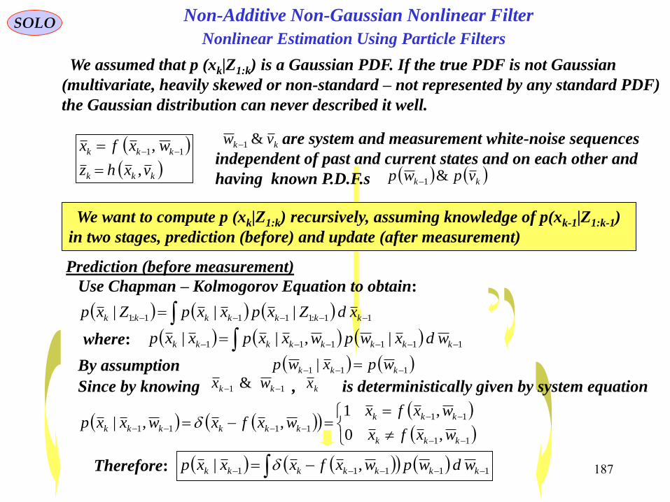
187
Nonlinear Estimation Using Particle FiltersSOLO
We assumed that p (xk|Z1:k) is a Gaussian PDF. If the true PDF is not Gaussian
(multivariate, heavily skewed or non-standard – not represented by any standard PDF)
the Gaussian distribution can never described it well.
Non-Additive Non-Gaussian Nonlinear Filter
kkk
kkk
vxhz
wxfx
,
, 11
kk vw &1 are system and measurement white-noise sequences
independent of past and current states and on each other and
having known P.D.F.s kk vpwp &1
We want to compute p (xk|Z1:k) recursively, assuming knowledge of p(xk-1|Z1:k-1)
in two stages, prediction (before) and update (after measurement)
Prediction (before measurement)
Use Chapman – Kolmogorov Equation to obtain:
11:1111:1 ||| kkkkkkk xdZxpxxpZxp
where: 111111 |,|| kkkkkkkk wdxwpwxxpxxp
By assumption 111 | kkk wpxwp
Since by knowing , is deterministically given by system equation11 & kk wx kx
11
11
1111,0
,1,,|
kkk
kkk
kkkkkkwxfx
wxfxwxfxwxxp
Therefore: 11111 ,| kkkkkkk wdwpwxfxxxp
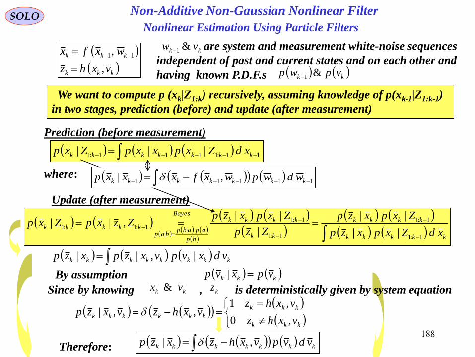
188
Nonlinear Estimation Using Particle FiltersSOLO Non-Additive Non-Gaussian Nonlinear Filter
kkk
kkk
vxhz
wxfx
,
, 11
kk vw &1 are system and measurement white-noise sequences
independent of past and current states and on each other and
having known P.D.F.s kk vpwp &1
We want to compute p (xk|Z1:k) recursively, assuming knowledge of p(xk-1|Z1:k-1)
in two stages, prediction (before) and update (after measurement)
Prediction (before measurement)
11:1111:1 ||| kkkkkkk xdZxpxxpZxp
where:
Update (after measurement)
kkkkk
kkkk
kk
kkkkBayes
bp
apabpbap
kkkkkxdZxpxzp
Zxpxzp
Zzp
ZxpxzpZzxpZxp
1:1
1:1
1:1
1:1
||
1:1:1||
||
|
||,||
kkkkkkkk vdxvpvxzpxzp |,||
By assumption kkk vpxvp |
Since by knowing , is deterministically given by system equationkk vx & kz
kkk
kkk
kkkkkkvxhz
vxhzvxhzvxzp
,0
,1,,|
Therefore: kkkkkkk vdvpvxhzxzp ,|
11111 ,| kkkkkkk wdwpwxfxxxp

189
Nonlinear Estimation Using Particle FiltersSOLO Non-Additive Non-Gaussian Nonlinear Filter
kkk
kkk
vxhz
wxfx
,
, 11
kk vw &1 are system and measurement white-noise sequences
independent of past and current states and on each other and
having known P.D.F.s kk vpwp &1
We want to compute p (xk|Z1:k) recursively, assuming knowledge of p(xk-1|Z1:k-1)
in two stages, prediction (before) and update (after measurement)
Prediction (before measurement) 11:1111:1 ||| kkkkkkk xdZxpxxpZxp
11111 ,| kkkkkkk wdwpwxfxxxp
Update (after measurement)
kkkkk
kkkk
kk
kkkkBayes
bp
apabpbap
kkkkkxdZxpxzp
Zxpxzp
Zzp
ZxpxzpZzxpZxp
1:1
1:1
1:1
1:1
||
1:1:1||
||
|
||,||
We need to evaluate the following integrals:
kkkkkkk vdvpvxhzxzp ,|
We use the numeric Monte Carlo Method to evaluate the integrals:
Generate (Draw): Sk
i
kk
i
k Nivpvwpw ,,1~&~ 11
S
N
i
i
k
i
k
i
kkk NwxfxxxpS
1
111 /,|
S
N
i
i
k
i
k
i
kkk NvxhzxzpS
1
/,|
or
S
N
i
i
kkkk
i
k
i
k
i
k NxxxxpwxfxS
1
111 /|,
S
N
i
i
kkkk
i
k
i
k
i
k NzzxzpvxhzS
1
/|,
Analytic solutions for those integral
equations do not exist in the general
case.

190
SOLO
kvkkk
xkkwkkkk
vpgivenvxhz
xpuwpgivenwuxfx
:,
,,:,, 011111 0
Monte Carlo Computations of and . kk xzp | 1| kk xxp
Generate (Draw) Sx
iNixpx ,,1~ 00 0
For ,,1k
Initialization0
1 At stage k-1
Generate (Draw) NS samples Skw
i
k Niwpw ,,1~ 11
2 State Update S
i
kk
i
k
i
k Niwuxfx ,,1,, 111
3 Generate (Draw) Measurement Noise Skv
i
k Nivpv ,,1~
k:=k+1 & return to 1
SN
i
S
i
kkkk Nxxxxp1
1 /|
SN
i
S
i
kkkk Nzzxzp1
/|
4 Measurement , Update S
i
k
i
k
i
k Nivxhz ,,1, kz
Nonlinear Estimation Using Particle Filters
Non-Additive Non-Gaussian Nonlinear Filter

191
Nonlinear Estimation Using Particle FiltersSOLO Non-Additive Non-Gaussian Nonlinear Filter
kkk
kkk
vxhz
wxfx
,
, 11
kk vw &1 are system and measurement white-noise sequences
independent of past and current states and on each other and
having known P.D.F.s kk vpwp &1
We want to compute p (xk|Z1:k) recursively, assuming knowledge of p(xk-1|Z1:k-1)
in two stages, prediction (before) and update (after measurement)
Prediction (before measurement) 11:1111:1 ||| kkkkkkk xdZxpxxpZxp
Update (after measurement)
kkkkk
kkkk
kk
kkkkBayes
bp
apabpbap
kkkkkxdZxpxzp
Zxpxzp
Zzp
ZxpxzpZzxpZxp
1:1
1:1
1:1
1:1
||
1:1:1||
||
|
||,||
We use the numeric Monte Carlo Method to evaluate the integrals:
Generate (Draw): Sk
i
kk
i
k Nivpvwpw ,,1~&~ 11
S
N
i
i
kkkk
i
k
i
k
i
k NxxxxpwxfxS
1
111 /|,
S
N
i
i
kkkk
i
k
i
k
i
k NzzxzpvxhzS
1
/|,
SSS N
i
i
kk
S
N
i
kkk
i
kk
S
k
N
i
kk
i
kk
S
kk xxN
xdZxpxxN
xdZxpxxN
Zxp11
1
11:111
1
1:111:1
1|
1|
1|
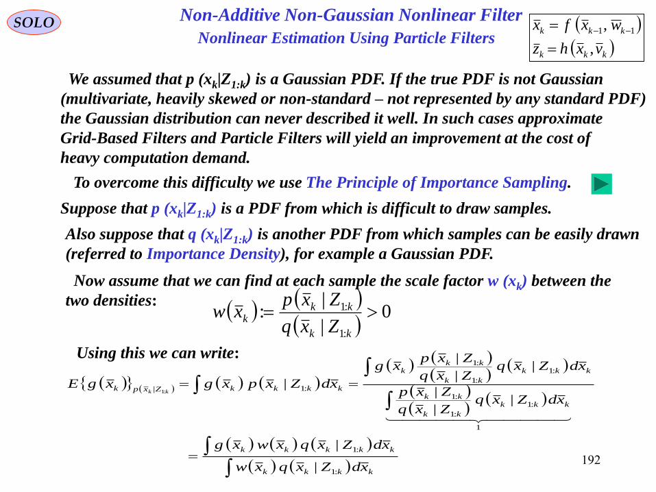
192
Nonlinear Estimation Using Particle FiltersSOLO
We assumed that p (xk|Z1:k) is a Gaussian PDF. If the true PDF is not Gaussian
(multivariate, heavily skewed or non-standard – not represented by any standard PDF)
the Gaussian distribution can never described it well. In such cases approximate
Grid-Based Filters and Particle Filters will yield an improvement at the cost of
heavy computation demand.
0|
|:
:1
:1 kk
kkk
Zxq
Zxpxw
To overcome this difficulty we use The Principle of Importance Sampling.
Suppose that p (xk|Z1:k) is a PDF from which is difficult to draw samples.
Also suppose that q (xk|Z1:k) is another PDF from which samples can be easily drawn
(referred to Importance Density), for example a Gaussian PDF.
Now assume that we can find at each sample the scale factor w (xk) between the
two densities:
Using this we can write:
kkkk
kkkkk
kkk
kk
kk
kkk
kk
kkk
kkkkZxpk
xdZxqxw
xdZxqxwxg
xdZxqZxq
Zxp
xdZxqZxq
Zxpxg
xdZxpxgxgEkk
:1
:1
1
:1
:1
:1
:1
:1
:1
:1|
|
|
||
|
||
|
|:1
Non-Additive Non-Gaussian Nonlinear Filter
kkk
kkk
vxhz
wxfx
,
, 11

193
SOLO
kkkk
kkkkk
ZxpkxdZxqxw
xdZxqxwxgxgE
kk
:1
:1
||
|
:1
sN
i
i
k
s
i
ki
k
xwN
xwxw
1
1:~
where
Generate (draw) Ns particle samples { xki, i=1,…,Ns } from q(xk|Z1:k)
skk
i
k NiZxqx ,,1|~ :1
s
s
s
kk
N
i
i
kkN
i
i
k
s
N
i
i
kk
s
Zxpk xwxg
xwN
xwxgN
xgE1
1
1
|
~
1
1
:1
and estimate g(xk) using a Monte Carlo approximation:
Nonlinear Estimation Using Particle Filters
Non-Additive Non-Gaussian Nonlinear Filter
kkk
kkk
vxhz
wxfx
,
, 11
Importance Sampling (IS)
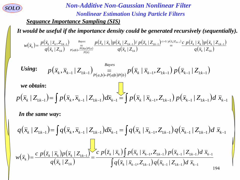
194
Nonlinear Estimation Using Particle FiltersSOLO
It would be useful if the importance density could be generated recursively (sequentially).
kk
kkkkZzpc
kk
kkkkkk
bP
aPabPbaP
Bayes
kk
kkkk
Zxq
Zxpxzpc
Zxq
ZzpZxpxzp
Zxq
Zzxpxw
kk
:1
1:1|/1:
:1
1:11:1
||:1
1:1
|
||
|
|/||
|
,| 1:1
1:111:11|,
1:11 |,||,
kkkkkbPbaPbaP
Bayes
kkk ZxpZxxpZxxpUsing:
we obtain:
11:111:1111:111:1 |,||,| kkkkkkkkkkkk xdZxpZxxpxdZxxpZxp
11:111:1111:111:1 |,||,| kkkkkkkkkkkk xdZxqZxxqxdZxxqZxq
In the same way:
11:111:11
11:111:11
:1
1:1
|,|
|,||
|
||
kkkkkk
kkkkkkkk
kk
kkkkk
xdZxqZxxq
xdZxpZxxpxzpc
Zxq
Zxpxzpcxw
Sequance Importance Sampling (SIS)
Non-Additive Non-Gaussian Nonlinear Filter

195
Nonlinear Estimation Using Particle Filters
SOLO
It would be useful if the importance density could be generated recursively.
11:111:11
11:111:11
:1
1:1
|,|
|,||
|
||
kkkkkk
kkkkkkkk
kk
kkkkk
xdZxqZxxq
xdZxpZxxpxzpc
Zxq
Zxpxzpcxw
Suppose that at k-1 we have Ns particle samples and their probabilities
{ xk-1|k-1i,wk-1
i ,i=1,…,Ns }, that constitute a random measure which characterizes the
posterior PDF for time up to tk-1. Then
sN
i
i
kkkk
i
kkkk xxZxpZxp1
1|111:11|11:11 ||
s
s
N
i
i
kkkk
i
kkkkk
k
N
i
i
kkkk
i
kkkkkkk
k
xxZxqZxxq
xdxxZxpZxxpxzpc
xw
1
1|111:11|11:11
1
1
1|111:11|11:11
|,|
|,||
sN
i
i
kkkk
i
kkkk xxZxqZxq1
1|111:11|11:11 ||
Sequential Importance Sampling (SIS) (continue – 1)
We obtained:
Non-Additive Non-Gaussian Nonlinear Filter

196
Nonlinear Estimation Using Particle Filters
SOLO
kk
kkkkBayes
kk
kkk
Zxq
Zxpxzpc
Zxq
Zxpxw
:1
1:1
:1
:1
|
||
|
|
1:11|11|1
1:11|11|1|,|
|,|
1:11|11:11|1
1:11|11:11|1
1
1|111:11|11:11
1
1
1|111:11|11:11
||
|||
|,|
|,||
|,|
|,||
1|11:11|1
1|11:11|1
k
i
kk
i
kkk
k
i
kk
i
kkkkkxxpZxxp
xxqZxxq
k
i
kkk
i
kkk
k
i
kkk
i
kkkkk
N
i
i
kkkk
i
kkkkk
k
N
i
i
kkkk
i
kkkkkkk
k
Zxqxxq
Zxpxxpxzpc
ZxqZxxq
ZxpZxxpxzpc
xxZxqZxxq
xdxxZxpZxxpxzpc
xw
ikkkk
ikkk
ikkkk
ikkk
s
s
1:11
1:111
|
|
kk
kkk
Zxq
ZxpxwSince
i
kk
i
kk
i
kk
i
kk
i
kkki
k
i
kxxq
xxpxzpcww
1|1|
1|1||
1|
||
Define k
i
kk
k
i
kki
kk
i
kZxq
Zxpxww
:1|
:1|
||
|:
1:11|1
1:11|1
1|11|
|:
k
i
kk
k
i
kki
kk
i
kZxq
Zxpxww
Sequential Importance Sampling (SIS) (continue – 2)
Non-Additive Non-Gaussian Nonlinear Filter
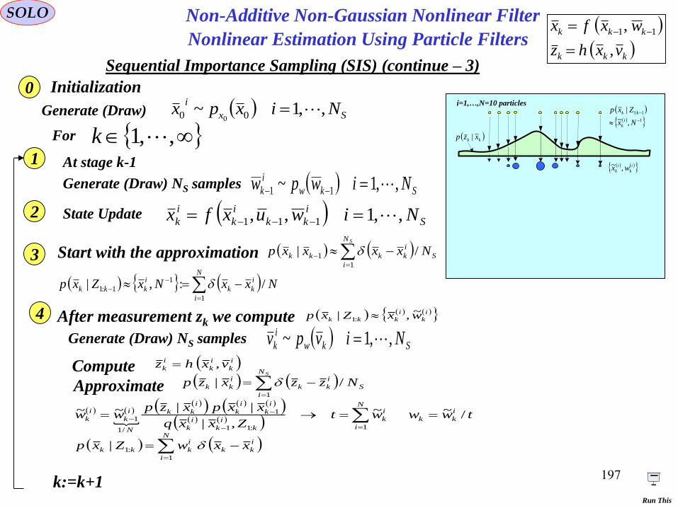
197
1
1:1
,~
|
Nx
Zxp
i
k
kk
i=1,…,N=10 particles
kk xzp |
SOLO
Sequential Importance Sampling (SIS) (continue – 3)
twwwtZxxq
xxpxzpww i
kk
N
i
i
k
k
i
k
i
k
i
k
i
k
i
kk
N
i
k
i
k /~~
,|
||~~
1:11
1
/1
1
N
i
i
kk
i
kkk NxxNxZxp1
1
1:1 /:,|
k:=k+1
1
1:1
,~
|
Nx
Zxp
i
k
kk
i
k
i
k wx ,~
i=1,…,N=10 particles
kk xzp |
Run This
Nonlinear Estimation Using Particle Filters
Non-Additive Non-Gaussian Nonlinear Filter
kkk
kkk
vxhz
wxfx
,
, 11
N
i
i
kk
i
kkk xxwZxp1
:1|
Generate (Draw) Sx
iNixpx ,,1~ 00 0
For ,,1k
Initialization0
1 At stage k-1
Generate (Draw) NS samples Skw
i
k Niwpw ,,1~ 11
2 State Update S
i
kk
i
k
i
k Niwuxfx ,,1,, 111
Start with the approximation
SN
i
S
i
kkkk Nxxxxp1
1 /| 3
After measurement zk we compute i
k
i
kkk wxZxp ~,| :1 4
Generate (Draw) NS samples Skw
i
k Nivpv ,,1~
Compute i
k
i
k
i
k vxhz ,
Approximate
SN
i
S
i
kk
i
kk Nzzxzp1
/|

198
Nonlinear Estimation Using Particle Filters
SOLO
The resulting sequential importance sampling (SIS) algorithm is a Monte Carlo method
that forms the basis for most sequential MC Filters.
Sequential Importance Sampling (SIS) (continue – 4)
This sequential Monte Carlo method is known variously as:
• Bootstrap Filtering
• Condensation Algorithm
• Particle Filtering
• Interacting Particle Approximation
• Survival of the Fittest
Non-Additive Non-Gaussian Nonlinear Filter
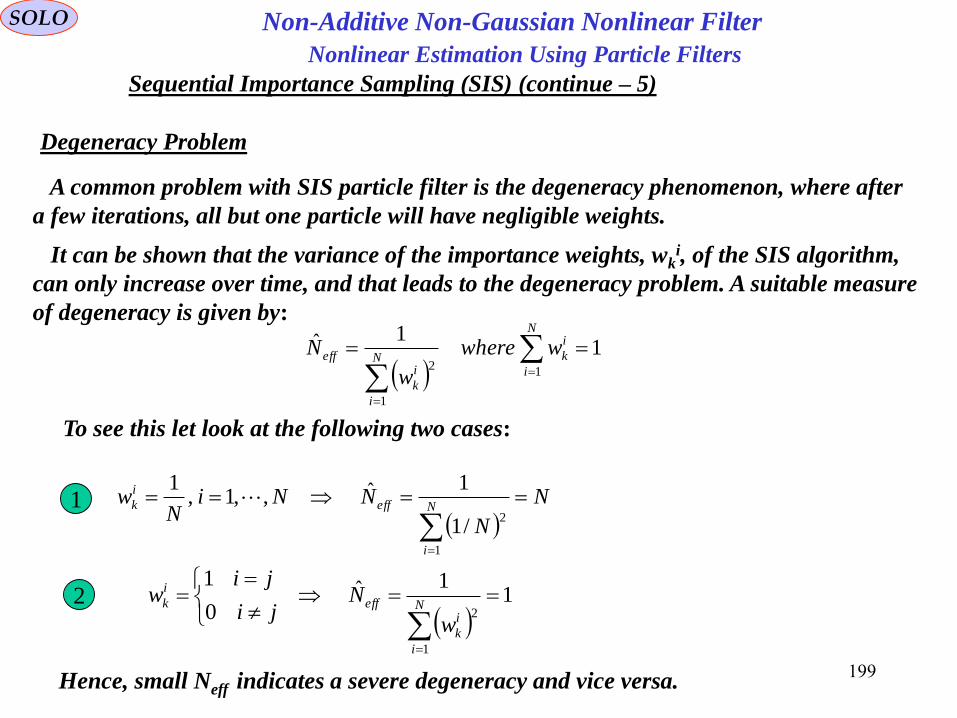
199
Nonlinear Estimation Using Particle Filters
SOLO
Degeneracy Problem
Sequential Importance Sampling (SIS) (continue – 5)
A common problem with SIS particle filter is the degeneracy phenomenon, where after
a few iterations, all but one particle will have negligible weights.
It can be shown that the variance of the importance weights, wki, of the SIS algorithm,
can only increase over time, and that leads to the degeneracy problem. A suitable measure
of degeneracy is given by:
1
1ˆ
1
1
2
N
i
i
kN
i
i
k
eff wwhere
w
N
To see this let look at the following two cases:
1
N
N
NNiN
wN
i
eff
i
k
1
2/1
1ˆ,,1,1
2
1
1ˆ0
1
1
2
N
i
i
k
eff
i
k
w
Nji
jiw
Hence, small Neff indicates a severe degeneracy and vice versa.
Non-Additive Non-Gaussian Nonlinear Filter
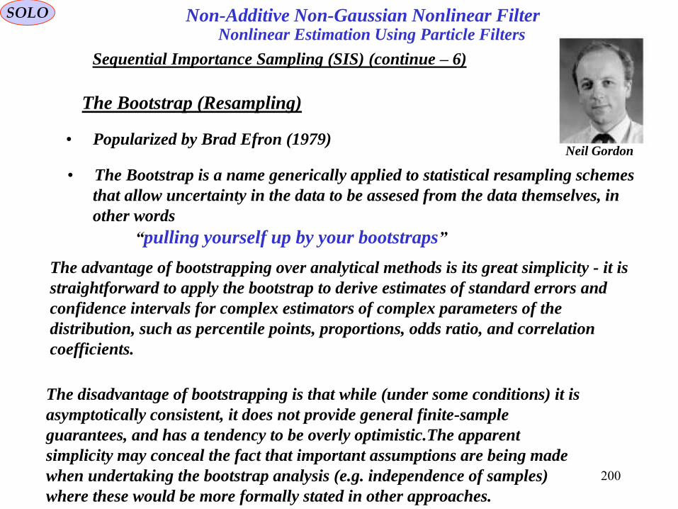
200
SOLO
The Bootstrap (Resampling)
• Popularized by Brad Efron (1979)
• The Bootstrap is a name generically applied to statistical resampling schemes
that allow uncertainty in the data to be assesed from the data themselves, in
other words
“pulling yourself up by your bootstraps”
The disadvantage of bootstrapping is that while (under some conditions) it is
asymptotically consistent, it does not provide general finite-sample
guarantees, and has a tendency to be overly optimistic.The apparent
simplicity may conceal the fact that important assumptions are being made
when undertaking the bootstrap analysis (e.g. independence of samples)
where these would be more formally stated in other approaches.
The advantage of bootstrapping over analytical methods is its great simplicity - it is
straightforward to apply the bootstrap to derive estimates of standard errors and
confidence intervals for complex estimators of complex parameters of the
distribution, such as percentile points, proportions, odds ratio, and correlation
coefficients.
Neil Gordon
Nonlinear Estimation Using Particle Filters
Sequential Importance Sampling (SIS) (continue – 6)
Non-Additive Non-Gaussian Nonlinear Filter

201
Nonlinear Estimation Using Particle Filters
j
C.D.F.
1
jkw~
0
SOLO
Resampling
Sequential Importance Sampling (SIS) (continue – 5)
Whenever a significant degeneracy is observed (i.e., when Neff falls bellow some
Threshold Nthr) during the sampling, where we obtained
N
i
i
kk
i
kkk xxwZxp1
:1|
we need to resample and replace the mapping representation
with a random measure
Niwx i
k
i
k ,,1,
NiNx i
k ,,1/1,*
This is done by first computing the Cumulative Density Function (C.D.F.) of the
sampled distribution wki.
Initialize the C.D.F.: c1 = wk1
Compute the C.D.F.: ci = ci-1 + wki
For i = 2:N
i := i + 1
Non-Additive Non-Gaussian Nonlinear Filter

202
ui
jresampled index
C.D.F.
11N
jkw~
0 0
SOLO
Resampling (continue – 1)
Sequential Importance Resampling (SIR) (continue – 2)
Using the method of Inverse Transform Algorithm we generate N independent and
identical distributed (i.i.d.) variables from the uniform distribution u, we sort them in
ascending order and we compare them with the Cumulative Distribution Function (C.D.F.)
of the normalized weights.
Nonlinear Estimation Using Particle Filters
Non-Additive Non-Gaussian Nonlinear Filter
kkk
kkk
vxhz
wxfx
,
, 11
Nonlinear Estimation Using Particle Filters
Non-Additive Non-Gaussian Nonlinear Filter
kkk
kkk
vxhz
wxfx
,
, 11
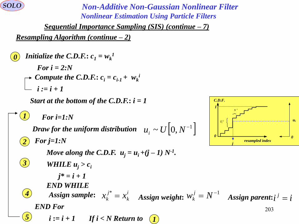
203
Nonlinear Estimation Using Particle Filters
ui
jresampled index
C.D.F.
11N
jkw~
0 0
SOLO
Resampling Algorithm (continue – 2)
Sequential Importance Sampling (SIS) (continue – 7)
Initialize the C.D.F.: c1 = wk1
Compute the C.D.F.: ci = ci-1 + wki
For i = 2:N
i := i + 1
0
Start at the bottom of the C.D.F.: i = 1
Draw for the uniform distribution 1,0~ NUui
1 For i=1:N
Move along the C.D.F. uj = ui +(j – 1) N-1.
For j=1:N2
WHILE uj > ci
j* = i + 1
END WHILE
3
END For
5 i := i + 1 If i < N Return to 1
4 Assign sample: i
k
j
k xx *Assign weight:
1 Nw j
k Assign parent: ii j
Non-Additive Non-Gaussian Nonlinear Filter

204
1
1:1
,
|
Nx
Zxp
i
k
kk
i=1,…,N=10 particles
kk xzp |
SOLO
Resampling
Sequential Importance Resampling (SIR) (continue – 4)
twwwt
Zxxq
xxpxzpww
i
kk
N
i
i
k
k
i
k
i
k
i
k
i
k
i
kk
N
i
k
i
k
/~~
,|
||~~
1
:11
1
/1
1
After measurement zk-1 we
compute i
k
i
kkk wxZxp ~,| :1
1
Start with the approximation
N
i
i
kk
i
kkk
Nxx
NxZxp
1
1
1:1
/:
,|
0
Prediction i
kk
i
k
i
k nuxfx ,,*1
to obtain 1
1:11 ,|
NxZxp i
kkk
3
k:=k+1
1
1:1
,
|
Nx
Zxp
i
k
kk
i
k
i
k wx ,
i=1,…,N=10 particles
kk xzp |
1
1:1
,
|
Nx
Zxp
i
k
kk
i
k
i
k wx ,
1,* Nx i
k
i=1,…,N=10 particles
kk xzp |
Resample
1
1:1
,
|
Nx
Zxp
i
k
kk
i
k
i
k wx ,
1,* Nx i
k
11,
Nx i
k
i=1,…,N=10 particles
kk xzp |
11 | kk xzp
Resample
1
1:1
,
|
Nx
Zxp
i
k
kk
i
k
i
k wx ,
1,* Nx i
k
11,
Nx i
k
i
k
i
k wx 11,
i=1,…,N=10 particles
kk xzp |
11 | kk xzp
Resample
Run This
Nonlinear Estimation Using Particle Filters
Non-Additive Non-Gaussian Nonlinear Filter
kkk
kkk
vxhz
wxfx
,
, 11
N
i
i
kk
i
kkk xxwZxp1
:1|
If Resample
to obtain 1
:1 ,*| NxZxp i
kkk
2 tht
N
i
i
keff NwN
1
2/1

205
Estimators
v
vxh ,z
x
Estimator
x
SOLO
The Cramér-Rao Lower Bound (CRLB) on the Variance of the Estimator
xE
- estimated mean vector
TTT
xxExExxExExxExE
2
- estimated variance matrix
For a good estimator we want
xxE
- unbiased estimator vector
TT
xxExExxE
2
- minimum estimation variance
Tk kzzZ 1: - the observation matrix after k observations
xkzzLxZL k ,,,1, - the Likelihood or the joint density function of Zk
We have:
Tp
zzzz ,,,21 T
nxxxx ,,,
21 T
pvvvv ,,,
21
The estimation of , using the measurements
of a system corrupted by noise is a random variable with
x x zv
dvvpxvZpxZpxZLv
k
vz
k
xz
k ;//,//
xbxZdxZLZx
kzdzdxkzzLkzzxkzzxE
kkk
,
1,,,1,,1,,1
- estimator bias xb
therefore:

206
Estimators
v
vxh ,z
x
Estimator
x
SOLO
The Cramér-Rao Lower Bound on the Variance of the Estimator (continue – 1)
xbxZdxZLZxZxE kkkk ,
We have:
x
xbZd
x
xZLZx
x
ZxE k
k
k
k
1
,
Since L [Zk,x] is a joint density function, we have:
1, kk ZdxZL
0
,,0
,
k
k
k
k
k
k
Zdx
xZLxZd
x
xZLxZd
x
xZL
x
xbZd
x
xZLxZx k
k
k
1
,
Using the fact that:
x
xZLxZL
x
xZL k
k
k
,ln,
,
x
xbZd
x
xZLxZLxZx k
k
kk
1
,ln,
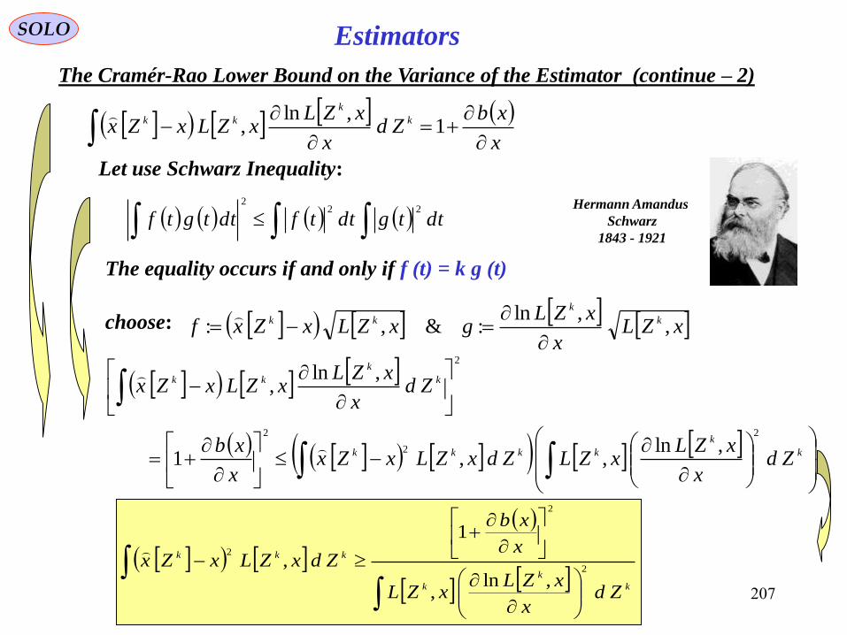
207
EstimatorsSOLO
The Cramér-Rao Lower Bound on the Variance of the Estimator (continue – 2)
x
xbZd
x
xZLxZLxZx k
k
kk
1
,ln,
Hermann Amandus
Schwarz
1843 - 1921
Let use Schwarz Inequality:
dttgdttfdttgtf22
2
The equality occurs if and only if f (t) = k g (t)
xZLx
xZLgxZLxZxf k
k
kk ,,ln
:&,:
choose:
k
k
kkkk
k
k
kk
Zdx
xZLxZLZdxZLxZx
x
xb
Zdx
xZLxZLxZx
2
2
2
2
,ln,,1
,ln,
k
k
k
kkk
Zdx
xZLxZL
x
xb
ZdxZLxZx2
2
2
,ln,
1
,

208
EstimatorsSOLO
The Cramér-Rao Lower Bound on the Variance of the Estimator (continue – 3)
k
k
k
kkk
Zdx
xZLxZL
x
xb
ZdxZLxZx2
2
2
,ln,
1
,
This is the Cramér-Rao bound for a biased estimator
Harald Cramér
1893 – 1985
Cayampudi Radhakrishna
Rao
1920 -
1,& kkk ZdxZLxbxZxE
1
2
0
2
22
,
,2,
,,
kk
kkkkkkkk
kkkkkkk
ZdxZLxb
ZdxZLZxEZxxbZdxZLZxEZx
ZdxZLxbZxEZxZdxZLxZx
xb
Zdx
xZLxZL
x
xb
ZdxZLZxEZx
k
k
k
kkkk
x
2
2
2
22
,ln,
1
,

209
EstimatorsSOLO
The Cramér-Rao Lower Bound on the Variance of the Estimator (continue – 4)
xb
Zdx
xZLxZL
x
xb
ZdxZLZxEZx
k
k
k
kkkk
x
2
2
2
22
,ln,
1
,
0,,ln
0,
1,,
,
,ln
kk
kxZL
x
xZL
x
xZL
k
k
kk ZdxZLx
xZLZd
x
xZLZdxZL
k
k
k
0,,ln,ln
,,ln
,
2
2
k
x
xZL
k
kk
kk
kx
ZdxZLx
xZL
x
xZLZdxZL
x
xZL
k
0
,ln,ln2
2
2
x
xZLE
x
xZLE
kkx
xb
x
xZLE
x
xb
xb
x
xZLE
x
xb
kk
x
2
2
2
2
2
2
2
2
,ln
1
,ln
1

210
Estimators
2
2
2
2
2
2
,ln
1
,ln
1
,
x
xZLE
x
xb
x
xZLE
x
xb
ZdxZLxZxk
k
kkk
SOLO
The Cramér-Rao Lower Bound on the Variance of the Estimator (continue – 5)
xb
x
xZLE
x
xb
xb
x
xZLE
x
xb
kk
x
2
2
2
2
2
2
2
2
,ln
1
,ln
1
For an unbiased estimator (b (x) = 0), we have:
2
22
2
,ln
1
,ln
1
x
xZLE
x
xZLE
kk
x
http://www.york.ac.uk/depts/maths/histstat/people/cramer.gif
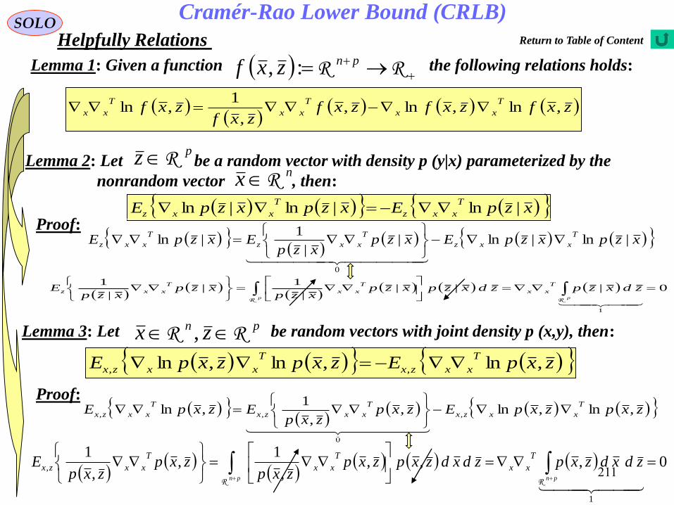
211
Cramér-Rao Lower Bound (CRLB)SOLO
Helpfully Relations
zxfzxfzxfzxf
zxfT
xx
T
xx
T
xx ,ln,ln,,
1,ln
Proof:
RR pnzxf :,Lemma 1: Given a function the following relations holds:
pz RLemma 2: Let be a random vector with density p (y|x) parameterized by the
nonrandom vector , then: nx R
xzpExzpxzpET
xxz
T
xxz |ln|ln|ln
xzpxzpExzpxzp
ExzpET
xxz
T
xxz
T
xxz |ln|ln||
1|ln
0
0|||
|
1|
|
1
1
pp
zdxzpzdxzpxzpxzp
xzpxzp
ET
xx
T
xx
T
xxz
RR
Proof:
zxpEzxpzxpET
xxzx
T
xxzx ,ln,ln,ln ,,
zxpzxpEzxpzxp
EzxpET
xxzx
T
xxzx
T
xxzx ,ln,ln,,
1,ln ,
0
,,
Lemma 3: Let be random vectors with joint density p (x,y), then: pn zx RR ,
0,,,
,
1,
,
1
1
,
pnpn
zdxdzxpzdxdzxpzxpzxp
zxpzxp
ET
xx
T
xx
T
xxzx
RR
Return to Table of Content

212
Cramér-Rao Lower Bound (CRLB)SOLO
Nonrandom Parameters
The Score of the estimation is defined by the logarithm of the likelihood xzpx |ln
In Maximum Likelihood Estimation (MLE), this function returns a vector valued
Score given by the observations and a candidate parameter vector .
Score close to zero are good scores since they indicate that is close to a local
optimum of , since
pz Rnx R
x xzp |
xzpxzp
xzp xx ||
1|ln
Since the measurement vector is stochastic the Expected Value of the Score
is given by:
pz R
0||||
|
1
||ln|ln
1
ppp
p
zdxzpzdxzpzdxzpxzpxzp
zdxzpxzpxzpE
xxx
xxz
RRR
R
v
vxh ,z
x
Estimator
x
The parameters are regarded as unknown but fixed.
The measurements are
nx Rpz R

213
Cramér-Rao Lower Bound (CRLB)
xzpExzpxzpExJT
xxz
T
xxz |ln|ln|ln:
SOLO
The Fisher Information Matrix (FIM)
Fisher, Sir Ronald Aylmer
1890 - 1962
The Fisher Information Matrix (FIM) was defined by Ronald Aylmer
Fisher as the Covariance Matrix of the Score
0||ln|ln p
zdxzpxpxzpE xxz
R
The Expected Value of the Score is given by:
The Covariance of the Score is given by:
p
zdxzpxzpxpxzpxzpET
xx
T
xxz
R
||ln|ln|ln|ln
Nonrandom Parameters
The Cramér-Rao Lower Bound on the Variance of the Estimator – Multivariable Case

214
Fisher, Sir Ronald Aylmer (1890-1962)
The Fisher information is the amount of information that
an observable random variable z carries about an unknown
parameter x upon which the likelihood of z, L(x) = f (Z; x),
depends. The likelihood function is the joint probability of
the data, the Zs, conditional on the value of x, as a function
of x. Since the expectation of the score is zero, the variance
is simply the second moment of the score, the derivative of
the lan of the likelihood function with respect to x. Hence
the Fisher information can be written
x
k
xxx
Tk
x
k
xxZLExZLxZLEx ,ln,ln,ln: J
Cramér-Rao Lower Bound (CRLB)
Return to Table of Content

215
Cramér-Rao Lower Bound (CRLB)SOLO
rxn
yy
T
y
Trxr
yy
T
yyz ytMyzpEJ RR **
:&|ln:
Nonrandom Parameters
The Likelihood p (z|x) may be over-parameterized so that some of x or combination of
elements of x do not affect p (z|x). In such a case the FIM for the parameters x becomes
singular. This leads to problems of computing the Cramér – Rao bounds. Let
(r ≤ n) be an alternative parameterization of the Likelihood such that p (z|y) is a well
defined density function for z given and the corresponding FIM is non-singular.
We define a possible non-invertible coordinate transformation .
ry R
ry R
ytx
Theorem 1: Nonrandom Parametric Cramér – Rao Bound
Assume that the observation has a well defined probability density function p (z|y)
for all , and let denote the parameter that yields the true distribution of .
Moreover, let be an Unbiased Estimator of , and let .
The estimation error covariance of is bounded for below by
pz Rry R *y y nzx Rˆ ytx ** ytx
zx
TT
z MJMxxxxE 1*ˆ*ˆ
where
are matrices that depend on the true unknown parameter vector .*y

216
Cramér-Rao Lower Bound (CRLB)SOLO
**
:&|ln:yy
T
y
T
yy
T
yyz ytMyzpEJ
Nonrandom Parameters
Theorem 1: Nonrandom Parametric Cramér – Rao Bound
Assume that the observation has a well defined probability density function p (z|y)
for all , and let denote the parameter that yields the true distribution of .
Moreover, let be an Unbiased Estimator of , and let .
The estimation error covariance of is bounded for below by
pz Rry R *y y nzx Rˆ ytx ** ytx
zx TT
z MJMxxxxE 1*ˆ*ˆ
where
are matrices that depend on the true unknown parameter vector .*y
Proof:
0|ˆ p
zdyzpytzxT
y
R
Tacking the gradient w.r.t. on both sides of this relation we obtain:y
0|ˆ| pp
zdyzpytzdytzxyzp T
y
T
y
RR
1
||ˆ|ln pp
zdyzpytzdyzpytzxyzp T
y
T
y
RR
ytzdyzpytzxyzp T
y
T
yp
R
|ˆ|ln
Consider the Random Vector:
yzp
xx
y |ln
ˆwhere:
0
0
|ln
ˆ
|ln
ˆ
yzpE
xxE
yzp
xxE
yz
z
y
z
0|ˆ|ˆˆ
sUnbiasenes
zxof
TT
pp
zdyzpytzxzdxzpxzx RR
Using the Unbiasedness of Estimator:

217
Cramér-Rao Lower Bound (CRLB)SOLO
**
:&|ln:yy
T
y
T
yy
T
yyz ytMyzpEJ
Nonrandom Parameters
Theorem 1: Nonrandom Parametric Cramér – Rao Bound
Assume that the observation has a well defined probability density function p (z|y)
for all , and let denote the parameter that yields the true distribution of .
Moreover, let be an Unbiased Estimator of , and let .
The estimation error covariance of is bounded for below by
pz Rry R *y y nzx Rˆ ytx ** ytx
zx TT
z MJMxxxxE 1*ˆ*ˆ
where
are matrices that depend on the true unknown parameter vector .*y
Proof (continue – 1):
Consider the Random Vector:
yzp
xx
y |ln
ˆ
The Covariance Matrix is Positive Semi-definite by construction:
0
0
|ln
ˆ
|ln
ˆ
yzpE
xxE
yzp
xxE
yz
z
y
z
0
0
0
0
0|ln
ˆ
|ln
ˆ
1
11 definiteSemiPositive
T
T
T
T
yy
zIMJ
I
J
MJMC
I
JMI
JM
MC
yzp
xx
yzp
xxE
T
z xxxxEC ˆˆ: yzpEyzpyzpEJT
yyz
T
yyz |ln|ln|ln:
ytxxyzpEM T
y
T
yz
T ˆ|ln:
TT
z
NotationsEquivalent
definiteSemiPositive
T MJMxxxxECMJMC 11 ˆˆ:0
ytzdyzpytzxyzp T
y
T
yp
R
|ˆ|lnWe found:
q.e.d.
where:

218
Cramér-Rao Lower Bound (CRLB)SOLO
nxn
yy
T
y
Tnxn
yy
T
yyz ybIMyzpEJ RR **
:&|ln:
Nonrandom Parameters
Corollary 1: Nonrandom Parametric Cramér – Rao Bound (Baiased Estimator)
Consider an estimaton problem defined by the likelihood p (y|z), and the fixed unknown
parameter . Any estimator with unknown bias has a mean square error
bounded from below by
*y zy yb
***ˆ*ˆ 1 ybybMJMyyyyE TTT
z
where
are matrices that depend on the true unknown parameter vector .*y
Proof:
Theorem 1 yields that:
Introduce the quantity , the estimator is an unbiased estimator of . ybyx : zyzx ˆˆ x
ybIyzpEybIxxxxE T
y
T
yyz
TT
y
T
z 1
|lnˆˆ
Using , we obtain: ybyx :
ybybybIyzpEybIyyyyE TT
y
T
yyz
TT
y
T
z 1
|lnˆˆ
after suitably inserting the true parameter .*y

219
Cramér-Rao Lower Bound (CRLB)
xbxb
x
xbI
x
xZLE
x
xbI
xbxbx
xbI
x
xZL
x
xZLE
x
xbI
xZxxZxEZdxZLxZxxZx
T
x
kT
T
x
Tkk
T
x
TkkkkTkk
1
2
2
1
,ln
,ln,ln
,
SOLO
The Cramér-Rao Lower Bound on the Variance of the Estimator
The multivariable form of the Cramér-Rao Lower Bound is:
n
k
n
k
k
xZx
xZx
xZx
11
n
k
k
kk
x
x
xZL
x
xZL
x
xZLxZL
,ln
,ln
,ln,ln
1
Fisher Information Matrix
x
k
x
Tkk
x
xZLE
x
xZL
x
xZLE
2
2 ,ln,ln,ln:J
Fisher, Sir Ronald Aylmer
1890 - 1962
Return to Table of Content

220
Cramér-Rao Lower Bound (CRLB)SOLO
Random Parameters
Theorem 2: Random Parameters (Posterior Cramér – Rao Bound)
p
zdyzpytxyb
R
|ˆ
rxnT
yz
TrxrT
yyyz ytEMyzpEJ RR :&,ln: ,where
then the Mean Square of the Estimate is Bounded from Below
ynrt RR : x
For Random Parameters there is no true parameter value. Instead, the prior assumption
on the parameter distribution determines the probability of different parameter vectors.
Like in the nonrandom parametric case, we assume a possible non-invertible mapping
between a parameter vector and the sought parameter . The vector
is assumed to have been chosen such that the joint probability density p (y,z) is a well
defined density.
y
Let be two random vectors with a well defined joint density
p (y,z), and let be an estimate of . If the estimator bias
pr zandy RR nzx Rˆ ytx
satisfies njandriallforypyb jzi
,,1,,10lim
TT
yz MJMxxxxE 1
,ˆˆ 0ˆˆ 1
,
definiteSemiPositive
TT
yz MJMxxxxE
Equivalent
Notations

221
Cramér-Rao Lower Bound (CRLB)SOLO
Random Parameters
Theorem 2: Random Parameters (Posterior Cramér – Rao Bound)
TT
yz MJMxxxxE 1
,ˆˆ ytEMyzpEJ T
yz
TT
yyyz :&,ln: ,
then the Mean Square of the Estimate is Bounded from Below
Proof:
Let be two random vectors with a well defined joint density
p (y,z), and let be an estimate of . If the estimator bias
pr zandy RR nzx Rˆ ytx
p
zdyzpytxyb
R
|ˆ and njandriallforypyb jzi
,,1,,10lim
Compute
ppp
zdytzxyzpzdyzpytzdypyzpytzxypybT
y
yp
T
y
yzp
T
y
T
y
RRR
ˆ,,|ˆ
,
Integrating both sides w.r.t. over its complete range Rr yieldsy
rprr
ydzdytzxyzpydypytydypybT
y
T
y
T
y
RRR
ˆ,
The (i,j) element of the left hand side matrix is:
riiiiyjyj
i
jydydydydydydypybypybyd
y
ypyb
rii
r
111
00
0
RR
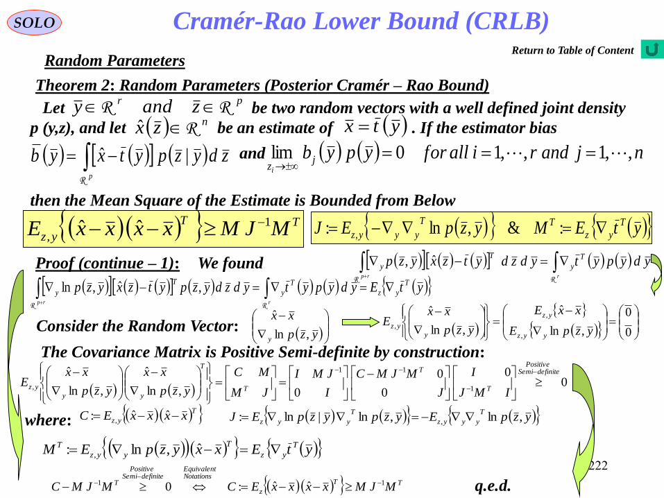
222
Cramér-Rao Lower Bound (CRLB)SOLO
Random Parameters
Theorem 2: Random Parameters (Posterior Cramér – Rao Bound)
TT
yz MJMxxxxE 1
,ˆˆ ytEMyzpEJ T
yz
TT
yyyz :&,ln: ,
then the Mean Square of the Estimate is Bounded from Below
Let be two random vectors with a well defined joint density
p (y,z), and let be an estimate of . If the estimator bias
pr zandy RR nzx Rˆ ytx
p
zdyzpytxyb
R
|ˆ and njandriallforypyb jzi
,,1,,10lim
Proof (continue – 1): We found rrp
ydypytydzdytzxyzp T
y
T
y
RR
ˆ,
ytEydypytydzdyzpytzxyzp T
yz
T
y
T
yrrp
RR
,ˆ,ln
Consider the Random Vector:
yzp
xx
y ,ln
ˆ
The Covariance Matrix is Positive Semi-definite by construction:
0
0
0
0
0,ln
ˆ
,ln
ˆ
1
11
,
definiteSemiPositive
T
T
T
T
yy
yzIMJ
I
J
MJMC
I
JMI
JM
MC
yzp
xx
yzp
xxE
ytExxyzpEM T
yz
T
yyz
T ˆ,ln: ,
TT
z
NotationsEquivalent
definiteSemiPositive
T MJMxxxxECMJMC 11 ˆˆ:0
q.e.d.
T
yz xxxxEC ˆˆ: , yzpEyzpyzpEJT
yyyz
T
yyz ,ln,ln|ln: , where:
0
0
,ln
ˆ
,ln
ˆ
,
,
,yzpE
xxE
yzp
xxE
yyz
yz
y
yz
Return to Table of Content

223
Cramér-Rao Lower Bound (CRLB)SOLO
Nonrandom and Random Parameters Cramér – Rao Bounds
For the Nonrandom Parameters the Cramér – Rao Bound depends on the true unknown
parameter vector y , and on the model of the problem defined by p (z|y) and the mapping
x = t (y). Hence the bound can only be computed by using simulations, when the true value
of the sought parameter vector y is known.
For the Random Parameters the Cramér – Rao Bound can be computed even in real
applications. Since the parameters are random there is no unknown true parameter value.
Instead, in the posterior Cramér – Rao Bound the matrices J and M are computed by
mathematical expectation performed with respect to the prior distribution of the parameters.
Return to Table of Content

224
Cramér-Rao Lower Bound (CRLB)SOLO
Discrete Time Nonlinear Estimation
p
kkk
n
kkk
vxhz
wxfx
R
R
,
, 11 kk vw &1 are system and measurement white-noise sequences
independent of past and current states and on each other and
having known P.D.F.s kk vpwp &1
0xpIn addition the P.D.F. of the initial state , is also given.
We found that the Cramér – Rao Lower Bound for the Random Parameters is given by:
1
:1:1,
1
:1:1:1:1,:1:1|:1:1:1|:1, ,ln,ln,ln:1:1:1:1
kk
T
XXZXkk
T
XkkXZX
T
kkkkkkZX XZpEXZpXZpEXXXXEkkkk
1 kk xfxIf we have a deterministic state model, i.e. then we can use the Nonrandom
Parametric Cramér – Rao Lower Bound
1
:1:1
1
:1:1:1:1:1:1|:1:1:1|:1 |ln|ln|ln:1:1:1:1
kk
T
XXZkk
T
XkkXZ
T
kkkkkkZ XZpEXZpXZpEXXXXEkkkk
After k cycles we have k measurements and k random parameters
estimated by an Unbiased Estimator as .
Tkk zzzZ ,,,: 21:1
Tkk xxxxX ,,,,: 210:0 Tkkkk xxxX |2|21|1:1|:1ˆ,,ˆ,ˆ:ˆ
The CRLB provides a lower bound for second-order (mean-squared) error only. Posterior
densities, which result from Nonlinear Filtering, are in general non-Gaussian. A full
statistical characterization of a non-Gaussian density requires higher order moments, in
addition to mean and covariance. Therefore, the CRLB for Nonlinear Filtering does not
fully characterize the accuracy of Filtering Algorithms.
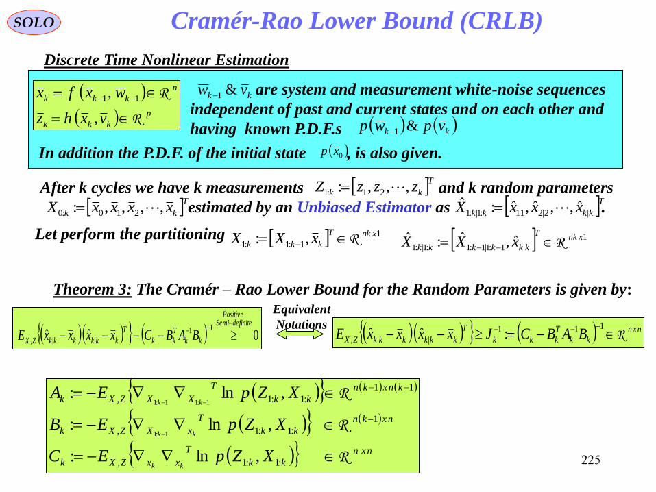
225
Cramér-Rao Lower Bound (CRLB)SOLO
Discrete Time Nonlinear Estimation
Theorem 3: The Cramér – Rao Lower Bound for the Random Parameters is given by:
Let perform the partitioning 1
1:1:1 ,: xnkT
kkk xXX R 1
|1:1|1:1:1|:1ˆ,ˆ:ˆ xnk
T
kkkkkk xXX R
p
kkk
n
kkk
vxhz
wxfx
R
R
,
, 11 kk vw &1 are system and measurement white-noise sequences
independent of past and current states and on each other and
having known P.D.F.s kk vpwp &1
0xpIn addition the P.D.F. of the initial state , is also given.
After k cycles we have k measurements and k random parameters
estimated by an Unbiased Estimator as .
Tkk zzzZ ,,,: 21:1
Tkk xxxxX ,,,,: 210:0 Tkkkk xxxX |2|21|1:1|:1ˆ,,ˆ,ˆ:ˆ
nxn
kk
T
xxZXk
nxkn
kk
T
xXZXk
knxkn
kk
T
XXZXk
XZpEC
XZpEB
XZpEA
kk
kk
kk
R
R
R
:1:1,
1
:1:1,
11
:1:1,
,ln:
,ln:
,ln:
1:1
1:11:1
nxn
kk
T
kkk
T
kkkkkkZX BABCJxxxxE R 111
||, :ˆˆ 0ˆˆ11
||,
definiteSemiPositive
kk
T
kk
T
kkkkkkZX BABCxxxxE
Equivalent
Notations

226
Cramér-Rao Lower Bound (CRLB)SOLO
Discrete Time Nonlinear Estimation
The Cramér – Rao Bound for the Random Parameters is given by:
0,ln,lnˆˆ
1
:1:1,:1:1,,
|
1:11:1|1:1
|
1:11:1|1:1
, 1:11:1
definiteSemiPositive
kk
T
xXkkxXZX
T
kkk
kkk
kkk
kkk
ZX XZpXZpExx
XX
xx
XXE
kkkk
Proof Theorem 3: Let perform the partitioning 1
1:1:1 ,: xnkT
kkk xXX R 1
|1:1|1:1:1|:1ˆ,ˆ:ˆ xnk
T
kkkkkk xXX R
1
:1:1,:1:1,
:1:1,:1:1,1
:1:1,,,
,ln,ln
,ln,ln,ln
1:1
1:11:11:1
1:11:1
kk
T
xxZXkk
T
XxZX
kk
T
xXZXkk
T
XXZX
kk
T
xXxXZX
XZpEXZpE
XZpEXZpEXZpE
kkkk
kkkk
kkkk
nkxnkkk
kk
T
kk
k
k
T
kk
T
k
kk
I
BAI
BABC
A
IAB
I
CB
BAR
11
11
1
00
00:
p
kkk
n
kkk
vxhz
wxfx
R
R
,
, 11 kk vw &1 are system and measurement white-noise sequences
independent of past and current states and on each other and
having known P.D.F.s kk vpwp &1
0xpIn addition the P.D.F. of the initial state , is also given.
After k cycles we have k measurements and k random parameters
estimated by an Unbiased Estimator as .
Tkk zzzZ ,,,: 21:1
Tkk xxxxX ,,,,: 210:0 Tkkkk xxxX |2|21|1:1|:1ˆ,,ˆ,ˆ:ˆ

227
Cramér-Rao Lower Bound (CRLB)SOLO
Discrete Time Nonlinear Estimation
0
0
0
0
0
ˆˆˆ
ˆ
1
111
111
||,1:11:1|1:1|,
|1:11:1|1:1,1:11:1|1:11:11:1|1:1,
definiteSemiPositive
k
T
kkk
T
kk
kkk
T
kkkkkkZX
T
kkkkkkZX
T
kkkkkkZX
T
kkkkkkZX
IAB
I
BABC
A
I
BAI
xxxxEXXxxE
xxXXEXXXXE
Proof Theorem 3 (continue – 1): We found
0
0
0
0
ˆˆˆ
ˆ
0
11
1
1
||,1:11:1|1:1|,
|1:11:1|1:1,1:11:1|1:11:11:1|1:1,1
definiteSemiPositive
kk
T
kk
k
k
T
kT
kkkkkkZX
T
kkkkkkZX
T
kkkkkkZX
T
kkkkkkZXkk
BABC
A
IAB
I
xxxxEXXxxE
xxXXEXXXXE
I
BAI
p
kkk
n
kkk
vxhz
wxfx
R
R
,
, 11 kk vw &1 are system and measurement white-noise sequences
independent of past and current states and on each other and
having known P.D.F.s kk vpwp &1
0xpIn addition the P.D.F. of the initial state , is also given.
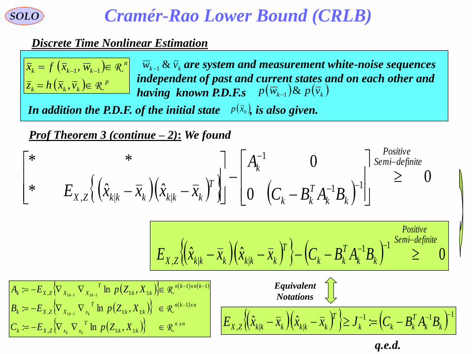
228
Cramér-Rao Lower Bound (CRLB)
111
||, :ˆˆ kk
T
kkk
T
kkkkkkZX BABCJxxxxE
SOLO
Discrete Time Nonlinear Estimation
Prof Theorem 3 (continue – 2): We found
0
0
0
ˆˆ*
**
11
1
||,
definiteSemiPositive
kk
T
kk
k
T
kkkkkkZX BABC
A
xxxxE
0ˆˆ11
||,
definiteSemiPositive
kk
T
kk
T
kkkkkkZX BABCxxxxE
Equivalent
Notations
nxn
kk
T
xxZXk
nxkn
kk
T
xXZXk
knxkn
kk
T
XXZXk
XZpEC
XZpEB
XZpEA
kk
kk
kk
R
R
R
:1:1,
1
:1:1,
11
:1:1,
,ln:
,ln:
,ln:
1:1
1:11:1
p
kkk
n
kkk
vxhz
wxfx
R
R
,
, 11 kk vw &1 are system and measurement white-noise sequences
independent of past and current states and on each other and
having known P.D.F.s kk vpwp &1
0xpIn addition the P.D.F. of the initial state , is also given.
q.e.d.
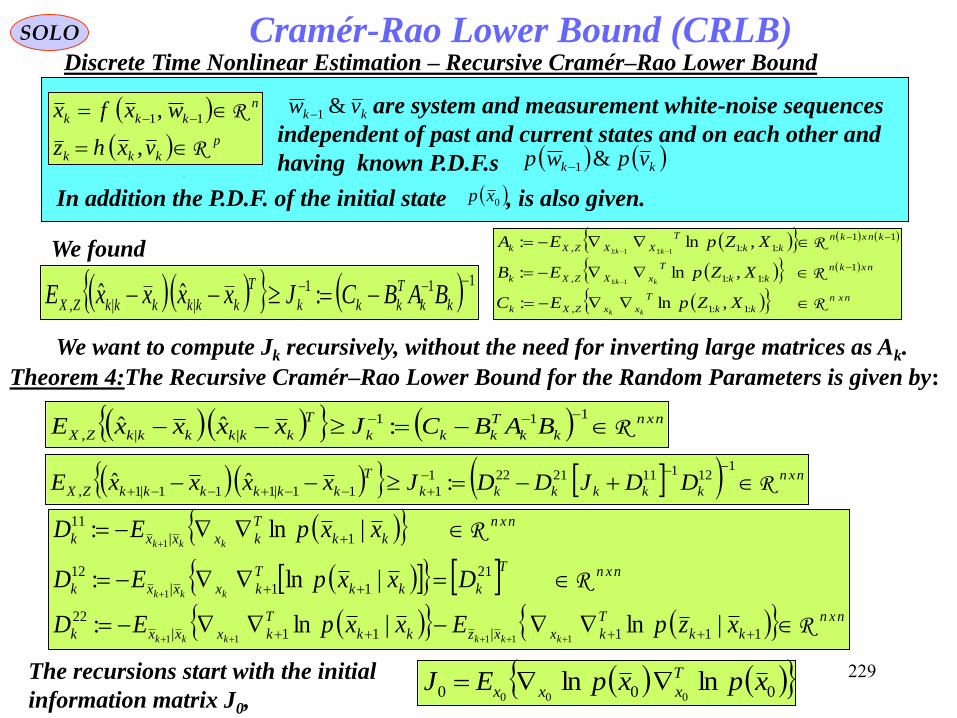
229
Cramér-Rao Lower Bound (CRLB)
nxn
kk
T
xxZXk
nxkn
kk
T
xXZXk
knxkn
kk
T
XXZXk
XZpEC
XZpEB
XZpEA
kk
kk
kk
R
R
R
:1:1,
1
:1:1,
11
:1:1,
,ln:
,ln:
,ln:
1:1
1:11:1
SOLO
Discrete Time Nonlinear Estimation – Recursive Cramér–Rao Lower Bound
We found
We want to compute Jk recursively, without the need for inverting large matrices as Ak.
111
||, :ˆˆ kk
T
kkk
T
kkkkkkZX BABCJxxxxE
p
kkk
n
kkk
vxhz
wxfx
R
R
,
, 11 kk vw &1 are system and measurement white-noise sequences
independent of past and current states and on each other and
having known P.D.F.s kk vpwp &1
0xpIn addition the P.D.F. of the initial state , is also given.
Theorem 4:The Recursive Cramér–Rao Lower Bound for the Random Parameters is given by:
nxn
kkkkkk
T
kkkkkkZX DDJDDJxxxxE R
11211121221
111|111|1, :ˆˆ
nxn
kk
T
kkk
T
kkkkkkZX BABCJxxxxE R 111
||, :ˆˆ
nxn
kk
T
kxxzkk
T
kxxxk
nxnT
kkk
T
kxxxk
nxn
kk
T
kxxxk
xzpExxpED
DxxpED
xxpED
kkkkkk
kkk
kkk
R
R
R
111|11|
22
21
11|
12
1|
11
|ln|ln:
|ln:
|ln:
11111
1
1
000 lnln000
xpxpEJ T
xxx The recursions start with the initial
information matrix J0,

230
Cramér-Rao Lower Bound (CRLB)SOLO
kk
T
xxZXk
kk
T
xXZXk
kk
T
XXZXk
XZpEC
XZpEB
XZpEA
kk
kk
kk
:1:1,
:1:1,
:1:1,
,ln:
,ln:
,ln:
1:1
1:11:1
We found
We want to compute Jk recursively, without the need for inverting large matrices as Ak.
111
||, :ˆˆ kk
T
kkk
T
kkkkkkZX BABCJxxxxE
Start with:
kkkkkkkkkkkkk XxZpXxZzpXxZzpXZp :11:1:11:11:11:111:11:1 ,,,,|,,,,
kk
xxpMarkov
kkk
xzpMarkov
kkkk XZpXZxpXxZzp
kkkk
:1:1
|
:1:11
|
:11:11 ,,|,,|
111
1:11:11 ,|| kkkkkk XZpxxpxzp
p
kkk
n
kkk
vxhz
wxfx
R
R
,
, 11 kk vw &1 are system and measurement white-noise sequences
independent of past and current states and on each other and
having known P.D.F.s kk vpwp &1
0xpIn addition the P.D.F. of the initial state , is also given.
Proof of Theorem 4:
Discrete Time Nonlinear Estimation – Recursive Cramér–Rao Lower Bound

231
Cramér-Rao Lower Bound (CRLB)
1
1
1
111
111
111
1
1:11:1,
11|1
|
1:11:1|1:1
11|1
|
1:11:1|1:1
, :,ln
ˆ
ˆ
ˆ
ˆ
1111:11
11:1
11:11:11:11:1
k
k
T
k
T
k
kk
T
k
kkk
kk
T
xx
T
xx
T
Xx
T
xx
T
xx
T
Xx
T
xX
T
xX
T
XX
ZX
T
kkk
kkk
kkk
kkk
kkk
kkk
ZX I
FEL
ECB
LBA
XZpE
xx
xx
XX
xx
xx
XX
E
kkkkkk
kkkkkk
kkkkkk
SOLO
Proof of Theorem 4 (continue – 1):
Compute:
kkkkkkkk XZpxxpxzpXZp :1:11111:11:1 ,||,
kkk
T
XXZX
kkkkkk
T
XXZXkk
T
XXZXk
AXZpE
XZpxxpxzpEXZpEA
kk
kkkk
:1:1,
:1:1111,1:11:1,1
,ln00
,ln|ln|ln,ln:
1:11:1
1:11:11:11:1
kkk
T
xXZX
kkkkkk
T
xXZXkk
T
xXZXk
BXZpE
XZpxxpxzpEXZpEB
kk
kkkk
:1:1,
:1:1111,1:11:1,1
,ln00
,ln|ln|ln,ln:
1:1
1:11:1
11
:1:1,1|
:1:1111,1:11:1,1
,ln|ln0
,ln|ln|ln,ln:
11
1 kk
C
kk
T
xxZX
D
kk
T
xxxx
kkkkkk
T
xxZXkk
T
xxZXk
DCXZpExxpE
XZpxxpxzpEXZpEC
k
kk
k
kkkk
kkkk
p
kkk
n
kkk
vxhz
wxfx
R
R
,
, 11 kk vw &1 are system and measurement white-noise sequences
independent of past and current states and on each other and
having known P.D.F.s kk vpwp &1
0xpIn addition the P.D.F. of the initial state , is also given.
Discrete Time Nonlinear Estimation – Recursive Cramér–Rao Lower Bound

232
Cramér-Rao Lower Bound (CRLB)
1
1
1
111
111
111
1
1:11:1,
11|1
|
1:11:1|1:1
11|1
|
1:11:1|1:1
, :,ln
ˆ
ˆ
ˆ
ˆ
1111:11
11:1
11:11:11:11:1
k
k
T
k
T
k
kk
T
k
kkk
kk
T
xx
T
xx
T
Xx
T
xx
T
xx
T
Xx
T
xX
T
xX
T
XX
ZX
T
kkk
kkk
kkk
kkk
kkk
kkk
ZX I
FEL
ECB
LBA
XZpE
xx
xx
XX
xx
xx
XX
E
kkkkkk
kkkkkk
kkkkkk
SOLO
Proof of Theorem 4 (continue – 2):
Compute:
kkkkkkkk XZpxxpxzpXZp :1:11111:11:1 ,||,
0,ln|ln|ln
,ln|ln|ln,ln:
0
:1:1,
0
1,
0
11,
:1:1111,1:11:1,1
11:111:111:1
11:111:1
kk
T
xXZXkk
T
xXZXkk
T
xXZX
kkkkkk
T
xXZXkk
T
xXZXk
XZpExxpExzpE
XZpxxpxzpEXZpEL
kkkkkk
kkkk
12
1|
0
:1:1,1,
0
11,
:1:1111,1:11:1,1
:|ln,ln|ln|ln
,ln|ln|ln,ln:
11111
11
kkk
T
xxxxkk
T
xxZXkk
T
xxZXkk
T
xxZX
kkkkkk
T
xxZXkk
T
xxZXk
DxxpEXZpExxpExzpE
XZpxxpxzpEXZpEE
kkkkkkkkkk
kkkk
22
0
:1:1,1|11|
:1:1111,1:11:1,1
,ln|ln|ln
,ln|ln|ln,ln:
111111111
1111
kkk
T
xxZXkk
T
xxxxkk
T
xxxz
kkkkkk
T
xxZXkk
T
xxZXk
DXZpExxpExzpE
XZpxxpxzpEXZpEF
kkkkkkkkkk
kkkk
p
kkk
n
kkk
vxhz
wxfx
R
R
,
, 11 kk vw &1 are system and measurement white-noise sequences
independent of past and current states and on each other and
having known P.D.F.s kk vpwp &1
0xpIn addition the P.D.F. of the initial state , is also given.
Discrete Time Nonlinear Estimation – Recursive Cramér–Rao Lower Bound
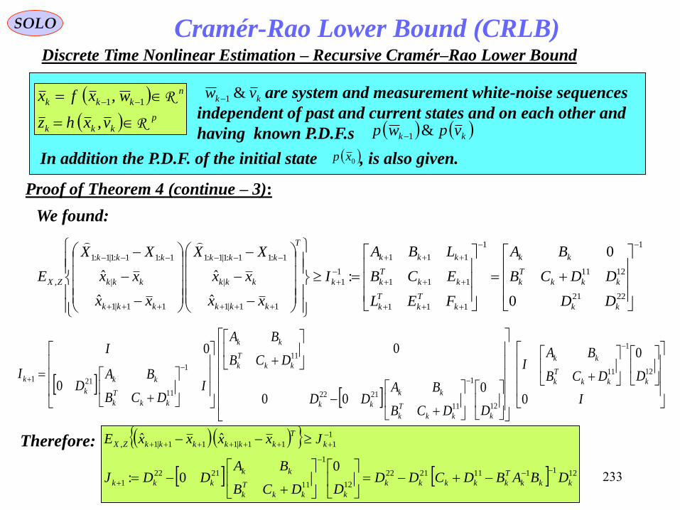
233
Cramér-Rao Lower Bound (CRLB)
1
2221
1211
1
111
111
111
1
1
11|1
|
1:11:1|1:1
11|1
|
1:11:1|1:1
,
0
0
:
ˆ
ˆ
ˆ
ˆ
kk
kkk
T
k
kk
k
T
k
T
k
kk
T
k
kkk
k
T
kkk
kkk
kkk
kkk
kkk
kkk
ZX
DD
DDCB
BA
FEL
ECB
LBA
I
xx
xx
XX
xx
xx
XX
E
SOLO
Proof of Theorem 4 (continue – 3):
We found:
I
DDCB
BAI
DDCB
BADD
DCB
BA
IDCB
BAD
I
Ikkk
T
k
kk
kkk
T
k
kk
kk
kk
T
k
kk
kk
T
k
kk
k
k
0
0
000
0
0
0
12
1
11
12
1
11
2122
11
1
11
211
Therefore:
1211112122
12
1
11
2122
1
1
111|111|1,
00:
ˆˆ
kkk
T
kkkkk
kkk
T
k
kk
kkk
k
T
kkkkkkZX
DBABDCDDDDCB
BADDJ
JxxxxE
p
kkk
n
kkk
vxhz
wxfx
R
R
,
, 11 kk vw &1 are system and measurement white-noise sequences
independent of past and current states and on each other and
having known P.D.F.s kk vpwp &1
0xpIn addition the P.D.F. of the initial state , is also given.
Discrete Time Nonlinear Estimation – Recursive Cramér–Rao Lower Bound

234
Cramér-Rao Lower Bound (CRLB)SOLO
The recursions start with the initial information matrix J0, which can be computed
from the initial density p (x0) as follows:
11211121221
111|111|1, :ˆˆ
kkkkkk
T
kkkkkkZX DDJDDJxxxxE
kk
T
xxZXk
kk
T
xXZXk
kk
T
XXZXk
XZpEC
XZpEB
XZpEA
kk
kk
kk
:1:1,
:1:1,
:1:1,
,ln:
,ln:
,ln:
1:1
1:11:1
Proof of Theorem 4 (continue – 4):
111
||, :ˆˆ kk
T
kkk
T
kkkkkkZX BABCJxxxxE
11|1|
22
21
1|
12
1|
11
|ln|ln:
|ln:
|ln:
1111111
11
1
kk
T
xxxzkk
T
xxxxk
T
kkk
T
xxxxk
kk
T
xxxxk
xzpExxpED
DxxpED
xxpED
kkkkkkkk
kkkk
kkkk
000 lnln000
xpxpEJ T
xxx
p
kkk
n
kkk
vxhz
wxfx
R
R
,
, 11 kk vw &1 are system and measurement white-noise sequences
independent of past and current states and on each other and
having known P.D.F.s kk vpwp &1
0xpIn addition the P.D.F. of the initial state , is also given.
Discrete Time Nonlinear Estimation – Recursive Cramér–Rao Lower Bound

235
Cramér-Rao Lower Bound (CRLB)SOLO
11211121221
111|111|1, :ˆˆ
kkkkkk
T
kkkkkkZX DDJDDJxxxxE
Proof of Theorem 4 (continue – 5):
nxn
kk
T
xxxzk
nxn
kk
T
xxxxk
kkk
nxnT
kkk
T
xxxxk
nxn
kk
T
xxxxk
xzpEDxxpED
DDD
DxxpED
xxpED
kkkkkkkk
kkkk
kkkk
RR
R
R
11|
22
1|
22
222222
21
1|
12
1|
11
|ln:2|ln:1
21:
|ln:
|ln:
1111111
11
1
p
kkk
n
kkk
vxhz
wxfx
R
R
,
, 11 kk vw &1 are system and measurement white-noise sequences
independent of past and current states and on each other and
having known P.D.F.s kk vpwp &1
0xpIn addition the P.D.F. of the initial state , is also given.
q.e.d.
tMeasuremenUpdated
22
ModelProcessUsingPrediction
121112122
1 21: kkkkkkk DDDJDDJ
Discrete Time Nonlinear Estimation – Recursive Cramér–Rao Lower Bound

236
Cramér-Rao Lower Bound (CRLB)SOLO
Discrete Time Nonlinear Estimation –Special Cases
00
1
000
0
0000ˆˆ
2
1exp
2
1,ˆ;
0xxPxx
PPxxxp
T
x
N
p
kkk
n
kkk
vxhz
wxfx
R
R
,
, 11 kk vw &1 are system and measurement white-noise sequences
independent of past and current states and on each other and
having known P.D.F.s kk vpwp &1
0xpIn addition the P.D.F. of the initial state , is also given.
Probability Density Function of is Gaussian0x
00
1
000
1
0000ˆˆˆ
2
1ln
000xxPxxPxxcxp
T
xxx
1
0
1
00
1
0
1
00000
1
0
1
00000
1
0000
ˆˆ
ˆˆlnln
0
000000
PPPPPxxxxEP
PxxxxPExpxpEJ
T
x
TT
xx
T
xxxx
Return to Table of Content

237
Cramér-Rao Lower Bound (CRLB)SOLO
Discrete Time Nonlinear Estimation –Special Cases
kkkk
T
kkk
k
kkkwkk xfxQxfxQ
Qwwpxxp 1
1
112
1exp
2
1,0;|
N
p
kkkk
n
kkkk
vxhz
wxfx
R
R
1111
1
1& kk vw are system and measurement Gaussian white-noise
sequences, independent of past and current states and on each
other with covariances Qk and Rk+1, respectively
0xpIn addition the P.D.F. of the initial state , is also given.
Additive Gaussian Noises
kkkkk
T
kxkkkk
T
kkkxkkx xfxQxfxfxQxfxcxxpkkk
1
1
1
1
112
1|ln
111
1
1111
1
111112
1exp
2
1,0;| kkkk
T
kkk
k
kkkvkk xhzRxhzR
Rvvpxzp
N
111
1
111111
1
1111211 111 2
1|ln
kkkkk
T
kxkkkk
T
kkkxkkx xhzRxhxhzRxhzcxzpkkk
11
11 11|ln
kk
T
kx
T
k
T
kxk
T
kkkxkk
T
xx QxfxfQxfxxxpkkkkk
Tk
T
kxk
T
k
T
kxk xhHxfFkk 111
:~
&:~
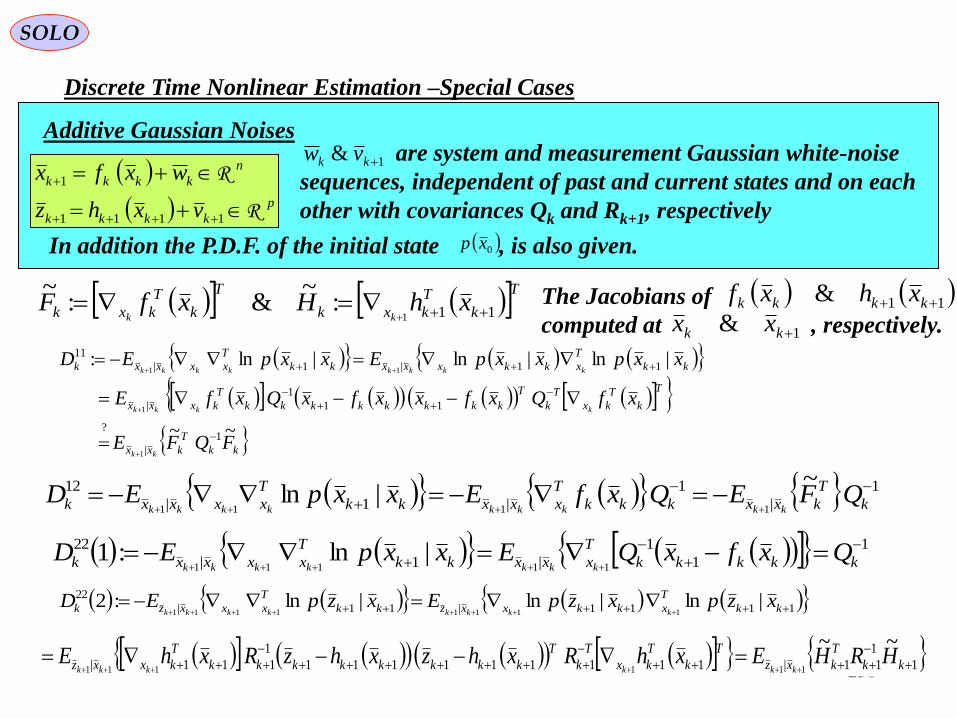
238
Cramér-Rao Lower Bound (CRLB)
SOLO
Discrete Time Nonlinear Estimation –Special Cases
p
kkkk
n
kkkk
vxhz
wxfx
R
R
1111
1
1& kk vw are system and measurement Gaussian white-noise
sequences, independent of past and current states and on each
other with covariances Qk and Rk+1, respectively
0xpIn addition the P.D.F. of the initial state , is also given.
Additive Gaussian Noises
11
11|111111111
1
111|
~~111111
kk
T
kxz
T
k
T
kx
T
k
T
kkkkkkkk
T
kxxz HRHExhRxhzxhzRxhEkkkkkk
1
|
1
|1|
12 ~|ln
1111
k
T
kxxkkk
T
xxxkk
T
xxxxk QFEQxfExxpEDkkkkkkkkk
Tk
T
kxk
T
k
T
kxk xhHxfFkk 111
:~
&:~
kk
T
kxx
T
k
T
kx
T
k
T
kkkkkkkk
T
kxxx
kk
T
xkkxxxkk
T
xxxxk
FQFE
xfQxfxxfxQxfE
xxpxxpExxpED
kk
kkkk
kkkkkkkk
~~
|ln|ln|ln:
1
|
?
11
1
|
11|1|
11
1
1
11
1111|11|
22 |ln|ln|ln:211111111
kk
T
xkkxxzkk
T
xxxzk xzpxzpExzpEDkkkkkkkk
The Jacobians of
computed at , respectively.
11& kkkk xhxf
1& kk xx
1
1
1
|1|
22
11111|ln:1
kkkkk
T
xxxkk
T
xxxxk QxfxQExxpEDkkkkkkk

239
Cramér-Rao Lower Bound (CRLB)
1
1
11|
22
122
1
|
12
1
|
11
~~2
1
~
~~
11
1
1
kk
T
kxzk
kk
k
T
kxxk
kk
T
kxxk
HRHED
QD
QFED
FQFED
kk
kk
kk
SOLO
Discrete Time Nonlinear Estimation –Special Cases
p
kkkk
n
kkkk
vxhz
wxfx
R
R
1111
1
1& kk vw are system and measurement Gaussian white-noise
sequences, independent of past and current states and on each
other with covariances Qk and Rk+1, respectively
0xpIn addition the P.D.F. of the initial state , is also given.
Additive Gaussian Noises
Tk
T
kxk
T
k
T
kxk xhHxfFkk 111
:~
&:~
The Jacobians of
computed at , respectively.
11& kkkk xhxf
1& kk xx
tMeasuremenUpdated
22
ModelProcessUsingPrediction
121112122
1 21: kkkkkkk DDDJDDJ
We can calculate the expectations using a Monte Carlo
Simulation. Using we draw 01 &, xpvpwp kk
Nivpvwpw
xpx
k
i
kk
i
k ,,2,1~&~
~
11
00
We Simulate System States and Measurements
Nivxhz
wxfx
i
k
i
kk
i
k
i
k
i
kk
i
k,,2,1
1111
1
We then average over realizations to get J0.
We average over realization to get next terms and so forth.0x
1x
Return to Table of Content
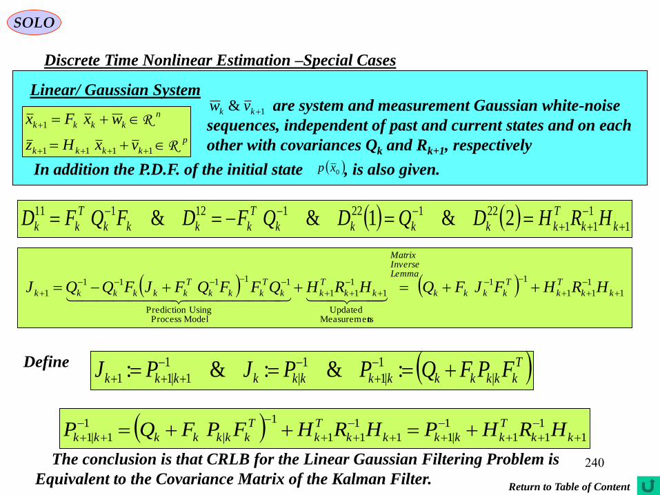
240
Cramér-Rao Lower Bound (CRLB)
1
1
11
22122112111 2&1&&
kk
T
kkkkk
T
kkkk
T
kk HRHDQDQFDFQFD
SOLO
Discrete Time Nonlinear Estimation –Special Cases
p
kkkk
n
kkkk
vxHz
wxFx
R
R
1111
1
1& kk vw are system and measurement Gaussian white-noise
sequences, independent of past and current states and on each
other with covariances Qk and Rk+1, respectively
0xpIn addition the P.D.F. of the initial state , is also given.
Linear/ Gaussian System
1
1
11
11
tsMeasuremenUpdated
1
1
11
ModelProcessUsingPrediction
11111
1
kk
T
k
T
kkkk
LemmaInverseMatrix
kk
T
kk
T
kkk
T
kkkkkk HRHFJFQHRHQFFQFJFQQJ
Define T
kkkkkkkkkkkkk FPFQPPJPJ |
1
|1
1
|
1
1|11 :&:&:
1
1
11
1
|11
1
11
1
|
1
1|1
kk
T
kkkkk
T
k
T
kkkkkkk HRHPHRHFPFQP
The conclusion is that CRLB for the Linear Gaussian Filtering Problem is
Equivalent to the Covariance Matrix of the Kalman Filter.Return to Table of Content
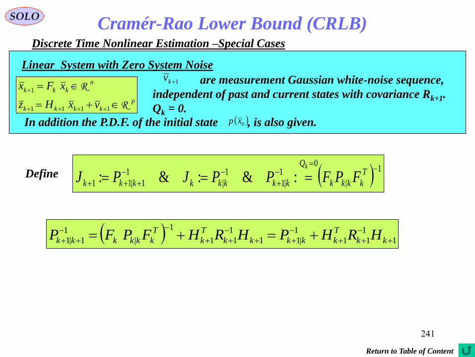
241
Cramér-Rao Lower Bound (CRLB)SOLO
Discrete Time Nonlinear Estimation –Special Cases
p
kkkk
n
kkk
vxHz
xFx
R
R
1111
1
1kv are measurement Gaussian white-noise sequence,
independent of past and current states with covariance Rk+1.
Qk = 0. 0xpIn addition the P.D.F. of the initial state , is also given.
Linear System with Zero System Noise
Define 1
|
01
|1
1
|
1
1|11 :&:&:
T
kkkk
Q
kkkkkkkk FPFPPJPJk
1
1
11
1
|11
1
11
1
|
1
1|1
kk
T
kkkkk
T
k
T
kkkkkk HRHPHRHFPFP
Return to Table of Content
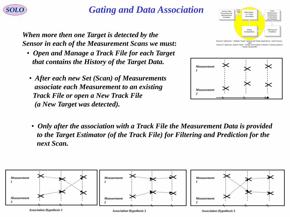
242
Sensor Data
Processing and
Measurement
Formation
Observation -
to - Track
Association
Input
DataTrack
Maintenance
) Initialization,
Confirmation
and Deletion(
Filtering and
Prediction
Gating
Computations
Samuel S . Blackman , " Multiple-Target Tracking with Radar Applications ", Artech House ,
1986Samuel S . Blackman , Robert Popoli , " Design and Analysis of Modern Tracking Systems
", Artech House , 1999
SOLO Gating and Data Association
Measurement
2
Measurement
1
t1 t2 t3
Association Hypothesis 1 Association Hypothesis 2 Association Hypothesis 3
Measurement
2
Measurement
1
t1 t2 t3
Measurement
2
Measurement
1
t1 t2 t3
Measurement
2
Measurement
1
t1 t2 t3
When more then one Target is detected by the
Sensor in each of the Measurement Scans we must:
• Open and Manage a Track File for each Target
that contains the History of the Target Data.
• After each new Set (Scan) of Measurements
associate each Measurement to an existing
Track File or open a New Track File
(a New Target was detected).
• Only after the association with a Track File the Measurement Data is provided
to the Target Estimator (of the Track File) for Filtering and Prediction for the
next Scan.

243
Sensor Data
Processing and
Measurement
Formation
Observation -
to - Track
Association
Input
DataTrack
Maintenance
) Initialization,
Confirmation
and Deletion(
Filtering and
Prediction
Gating
Computations
Samuel S . Blackman , " Multiple-Target Tracking with Radar Applications ", Artech House ,
1986Samuel S . Blackman , Robert Popoli , " Design and Analysis of Modern Tracking Systems
", Artech House , 1999
SOLO Gating and Data Association
Background
Filtering: deals with a Single Target, i.e.
Probability of Detection PD = 1, Probability of False Alarm PFA = 0
Facts:
• Sensors operate with PD < 1 and PFA > 0.
• Multiple Targets are often present.
• Measurements (plots) are not labeled!
Problem: How to know which measurements correspond to which Target (Track File)
The goal of Gating and Data Association:
Determine the origin of each Measurement by associating it to the existing Track File,
New Track File or declaring it to be a False Detection.

244
Sensor Data
Processing and
Measurement
Formation
Observation -
to - Track
Association
Input
DataTrack
Maintenance
) Initialization,
Confirmation
and Deletion(
Filtering and
Prediction
Gating
Computations
Samuel S . Blackman , " Multiple-Target Tracking with Radar Applications ", Artech House ,
1986Samuel S . Blackman , Robert Popoli , " Design and Analysis of Modern Tracking Systems
", Artech House , 1999
SOLO Gating and Data Association
Gating and Data Association Techniques
• Gating (Ellipsoidal, Rectangular, Others)
• (Global) Nearest Neighbor (GNN, NN) Algorithm
• Multiple Hypothesis Tracking (MHT)
• (Joint) Probabilistic Data Association (JPDA/PDA)
• Multidimensional Assignment
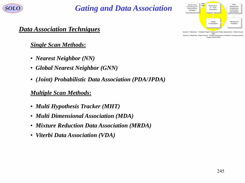
245
Sensor Data
Processing and
Measurement
Formation
Observation -
to - Track
Association
Input
DataTrack
Maintenance
) Initialization,
Confirmation
and Deletion(
Filtering and
Prediction
Gating
Computations
Samuel S . Blackman , " Multiple-Target Tracking with Radar Applications ", Artech House ,
1986Samuel S . Blackman , Robert Popoli , " Design and Analysis of Modern Tracking Systems
", Artech House , 1999
SOLO Gating and Data Association
Data Association Techniques
• Nearest Neighbor (NN)
Single Scan Methods:
• Global Nearest Neighbor (GNN)
• (Joint) Probabilistic Data Association (PDA/JPDA)
Multiple Scan Methods:
• Multi Hypothesis Tracker (MHT)
• Multi Dimensional Association (MDA)
• Mixture Reduction Data Association (MRDA)
• Viterbi Data Association (VDA)

246
Sensor Data
Processing and
Measurement
Formation
Observation -
to - Track
Association
Input
Data Track Maintenance
( Initialization,
Confirmation
and Deletion)
Filtering and
Prediction
Gating
Computations
Samuel S. Blackman, " Multiple-Target Tracking with Radar Applications", Artech House,
1986Samuel S. Blackman, Robert Popoli, " Design and Analysis of Modern Tracking Systems",
Artech House, 1999
11 , ktxz
12 kj tS
kkj ttz |ˆ11
12 , ktxz
13 , ktxz
kkj ttz |ˆ12
11 kj tS
Trajectory j = 2
Trajectory j = 1
Measurements
at scan k+1
SOLO
Optimal Correlation of Sensor Data with Tracks on
Surveillance Systems (R.G. Sea, Hughes, 1973)
We have n stored tracks that have predicted measurements
and innovations co variances at scan k+1 given by:
At scan k+1 we have m sensor reports (no more than one report
per target)
Gating and Data Association
njkSkkz jj ,,11,|1ˆ
set of all sensor reports on scan k+1 mk zzD ,,11
H – a particular hypothesis (from a complete set S of
hypotheses) connecting r (H) tracks to r measurements.
We want to solve the following Optimization Problem:
HPHDPcHPHDP
HPHDPDHPDHP
SH
SH
SHSH|max
1
|
|max|max|*
Measurement
2
Measurement
1
t1 t2 t3
Association Hypothesis 1
Measurement
2
Measurement
1
t1 t2 t3
Association Hypothesis 2
Measurement
2
Measurement
1
t1 t2 t3
Association Hypothesis 3
Measurement
2
Measurement
1
t1 t2 t3
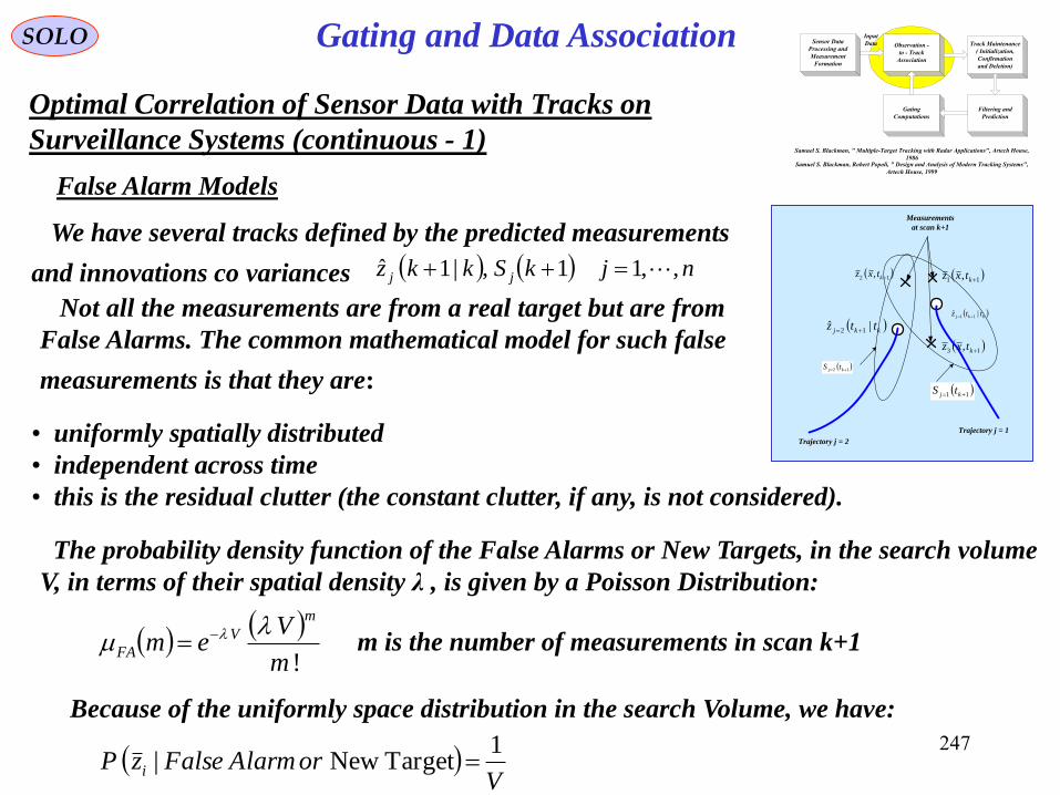
247
Sensor Data
Processing and
Measurement
Formation
Observation -
to - Track
Association
Input
Data Track Maintenance
( Initialization,
Confirmation
and Deletion)
Filtering and
Prediction
Gating
Computations
Samuel S. Blackman, " Multiple-Target Tracking with Radar Applications", Artech House,
1986Samuel S. Blackman, Robert Popoli, " Design and Analysis of Modern Tracking Systems",
Artech House, 1999
11 , ktxz
12 kj tS
kkj ttz |ˆ11
12 , ktxz
13 , ktxz
kkj ttz |ˆ12
11 kj tS
Trajectory j = 2
Trajectory j = 1
Measurements
at scan k+1
SOLO
Optimal Correlation of Sensor Data with Tracks on
Surveillance Systems (continuous - 1)
We have several tracks defined by the predicted measurements
and innovations co variances
Gating and Data Association
!m
Vem
m
V
FA
The probability density function of the False Alarms or New Targets, in the search volume
V, in terms of their spatial density λ , is given by a Poisson Distribution:
njkSkkz jj ,,11,|1ˆ
Not all the measurements are from a real target but are from
False Alarms. The common mathematical model for such false
measurements is that they are:
• uniformly spatially distributed
• independent across time
• this is the residual clutter (the constant clutter, if any, is not considered).
m is the number of measurements in scan k+1
V
orAlarmFalsezP i
1TargetNew|
Because of the uniformly space distribution in the search Volume, we have:
False Alarm Models
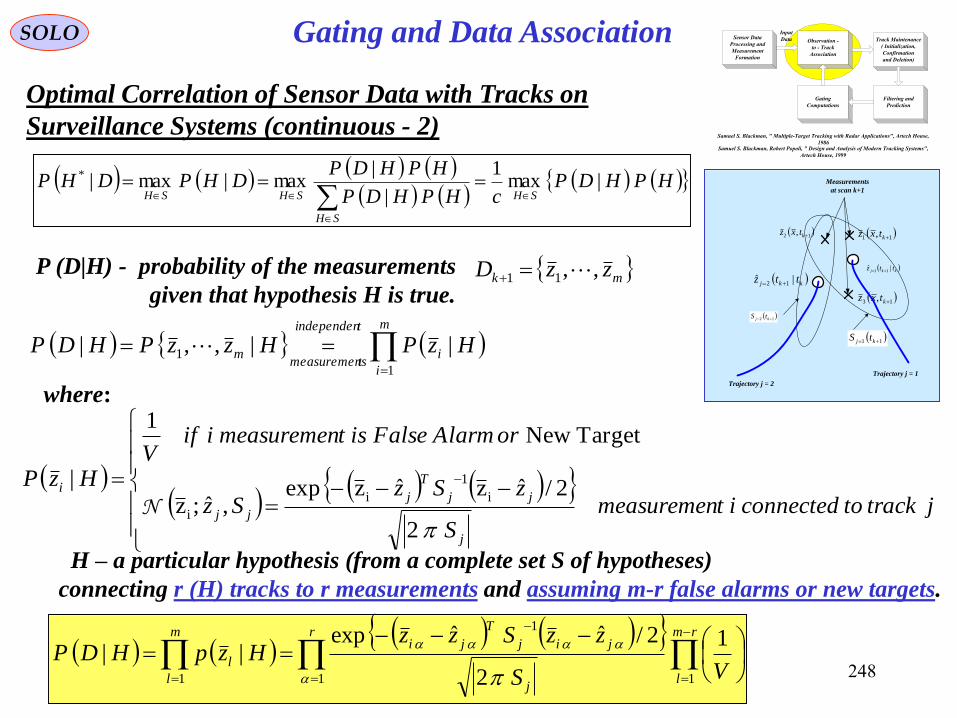
248
Sensor Data
Processing and
Measurement
Formation
Observation -
to - Track
Association
Input
Data Track Maintenance
( Initialization,
Confirmation
and Deletion)
Filtering and
Prediction
Gating
Computations
Samuel S. Blackman, " Multiple-Target Tracking with Radar Applications", Artech House,
1986Samuel S. Blackman, Robert Popoli, " Design and Analysis of Modern Tracking Systems",
Artech House, 1999
11 , ktxz
12 kj tS
kkj ttz |ˆ11
12 , ktxz
13 , ktxz
kkj ttz |ˆ12
11 kj tS
Trajectory j = 2
Trajectory j = 1
Measurements
at scan k+1
SOLO
Optimal Correlation of Sensor Data with Tracks on
Surveillance Systems (continuous - 2)
Gating and Data Association
mk zzD ,,11
H – a particular hypothesis (from a complete set S of hypotheses)
connecting r (H) tracks to r measurements and assuming m-r false alarms or new targets.
r rm
lj
jij
T
jim
l
lVS
zzSzzHzpHDP
1 1
1
1
1
2
2/ˆˆexp||
HPHDPcHPHDP
HPHDPDHPDHP
SH
SH
SHSH|max
1
|
|max|max|*
P (D|H) - probability of the measurements
given that hypothesis H is true.
m
i
i
tindependen
tsmeasuremenm HzPHzzPHDP
1
1 ||,,|
where:
jtracktoconnecteditmeasuremenS
zSzSz
orAlarmFalseistmeasuremeniifV
HzP
j
jj
T
j
jj
i
2
2/ˆzˆzexp,ˆ;z
TargetNew1
|i
1
i
iN

249
Sensor Data
Processing and
Measurement
Formation
Observation -
to - Track
Association
Input
Data Track Maintenance
( Initialization,
Confirmation
and Deletion)
Filtering and
Prediction
Gating
Computations
Samuel S. Blackman, " Multiple-Target Tracking with Radar Applications", Artech House,
1986Samuel S. Blackman, Robert Popoli, " Design and Analysis of Modern Tracking Systems",
Artech House, 1999
11 , ktxz
12 kj tS
kkj ttz |ˆ11
12 , ktxz
13 , ktxz
kkj ttz |ˆ12
11 kj tS
Trajectory j = 2
Trajectory j = 1
Measurements
at scan k+1
SOLO
Optimal Correlation of Sensor Data with Tracks on
Surveillance Systems (continuous - 3)
Gating and Data Association
HPHDPcHPHDP
HPHDPDHPDHP
SH
SH
SHSH|max
1
|
|max|max|*
P (H) – probability of hypothesis H connecting tracks j1,…,jr
to measurements i1,…,ir from m sensor reports:
mPrmPjjPjjiiPHP FA
tracks
r
tracks
r
tsmeasuremen
r
,,,,|,, 111
!
!
11
1,,|,, 11
m
rm
rmmmjjiiP
tracks
r
tsmeasuremen
r
probability of connecting tracks j1,…,jr
to measurements i1,…,ir
n
j
D
r
D
D
DetectingNot
n
jjjj
D
jjDetecting
r
D
tracks
r j
j
j
r
j
r
jP
P
PPPjjP
11,,
1
,,
1
1 11
1,,
1
1
probability of detecting only j1,…,jr
targets
V
rm
FAFA erm
VrmrmP
!
for (m-r) False Alarms or New Targets assume Poisson
Distribution with density λ over search volume V of
(m-r) reports
mP probability of exactly m reports
where:

250
Sensor Data
Processing and
Measurement
Formation
Observation -
to - Track
Association
Input
Data Track Maintenance
( Initialization,
Confirmation
and Deletion)
Filtering and
Prediction
Gating
Computations
Samuel S. Blackman, " Multiple-Target Tracking with Radar Applications", Artech House,
1986Samuel S. Blackman, Robert Popoli, " Design and Analysis of Modern Tracking Systems",
Artech House, 1999
11 , ktxz
12 kj tS
kkj ttz |ˆ11
12 , ktxz
13 , ktxz
kkj ttz |ˆ12
11 kj tS
Trajectory j = 2
Trajectory j = 1
Measurements
at scan k+1
SOLO
Optimal Correlation of Sensor Data with Tracks on
Surveillance Systems (continuous - 4)
where:
Gating and Data Association
HPHDPc
DHPDHPSHSH
|max1
|max|*
r
j
jij
T
ji
rmm
l
l
S
zzSzz
VHzpHDP
1
1
1 2
2/ˆˆexp1||
mPe
rm
VP
P
P
m
rmHP V
rmn
j
D
r
D
D
j
j
j
!1
1!
!
11
r
d
jij
T
ji
jD
D
const
n
j
D
Vm
ji
j
j
jzzSzz
SP
PPmPe
cHPHDP
c 1
1
12
ˆˆ2
1
1ln2
2
11
1ln|
1ln
jjiji
jD
D
d
jij
T
jijiSH
GdSP
PzzSzzHPHDP
cj
j
ji
2
,
1
,min
2
1
1ln2ˆˆmin|
1lnmax
2
jD
D
j
SP
PG
j
j
2
1
1ln2:

251
Sensor Data
Processing and
Measurement
Formation
Observation -
to - Track
Association
Input
Data Track Maintenance
( Initialization,
Confirmation
and Deletion)
Filtering and
Prediction
Gating
Computations
Samuel S. Blackman, " Multiple-Target Tracking with Radar Applications", Artech House,
1986Samuel S. Blackman, Robert Popoli, " Design and Analysis of Modern Tracking Systems",
Artech House, 1999
11 , ktxz
12 kj tS
kkj ttz |ˆ11
12 , ktxz
13 , ktxz
kkj ttz |ˆ12
11 kj tS
Trajectory j = 2
Trajectory j = 1
Measurements
at scan k+1
SOLO
Optimal Correlation of Sensor Data with Tracks on
Surveillance Systems (continuous - 5)
Gating and Data Association
HPHDPc
DHPDHPSHSH
|max1
|max|*
jji
jiGd
2
,min
jD
D
j
SP
PG
j
j
2
1
1ln2: Association Gate to track j
Return to Table of ContentInnovation in Tracking
In order to find the measurement that
nizzSzzd jij
T
jiji ,,1ˆˆ:12
belongs to track j, compute
jjiji
Gd 2
,minand choose i for which we have
mki zzDz ,,11

252
Sensor Data
Processing and
Measurement
Formation
Observation -
to - Track
Association
Input
DataTrack
Maintenance
) Initialization,
Confirmation
and Deletion(
Filtering and
Prediction
Gating
Computations
Samuel S . Blackman , " Multiple-Target Tracking with Radar Applications ", Artech House ,
1986Samuel S . Blackman , Robert Popoli , " Design and Analysis of Modern Tracking Systems
", Artech House , 1999
SOLO Gating and Data Association
Gating
• A way of simplifying data association by eliminating
unlikely observation-to-track pairings.
• We perform this test for every Target being tracked.
• Observation which don’t fall in any of the Gates will be used to initiate potentially
new tracks.
• We use the “measurement prediction” of the filter
1|1|ˆ,ˆ
kkkk xkhz
• Using we device a Gate around it, and dismiss
all the observations thatfall outside the Gate,
for data association.
1|ˆ
kkz
1|ˆ
kkz
1ktz Measurement
at tk-1
Measurement
Prediction
at tk
ktS
1|ˆ
kkz
ktxz ,1
ktS
1|ˆ
kkz
ktxz ,2
ktxz ,3
Nearest-Neighbor
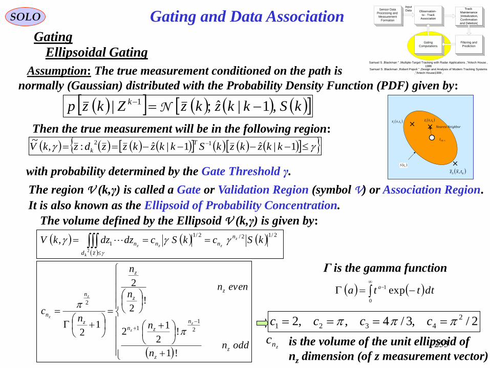
253
Sensor Data
Processing and
Measurement
Formation
Observation -
to - Track
Association
Input
DataTrack
Maintenance
) Initialization,
Confirmation
and Deletion(
Filtering and
Prediction
Gating
Computations
Samuel S . Blackman , " Multiple-Target Tracking with Radar Applications ", Artech House ,
1986Samuel S . Blackman , Robert Popoli , " Design and Analysis of Modern Tracking Systems
", Artech House , 1999
ktxz ,1
ktS
1|ˆ
kkz
ktxz ,2
ktxz ,3
Nearest-Neighbor
1|ˆ1|ˆ:,~ 12
kkzkzkSkkzkzzdzkVT
k
SOLO
Gating
Then the true measurement will be in the following region:
with probability determined by the Gate Threshold γ.
Gating and Data Association
Assumption: The true measurement conditioned on the path is
normally (Gaussian) distributed with the Probability Density Function (PDF) given by:
kSkkzkzZkzp k ,1|ˆ;| 1 N
The region V (k,γ) is called a Gate or Validation Region (symbol V) or Association Region.
It is also known as the Ellipsoid of Probability Concentration.
The volume defined by the Ellipsoid V (k,γ) is given by:
2/12/2/1
12
, kSckScdzdzkV z
zz
k
z
n
nn
zd
n
oddnn
n
evennn
n
nc
z
z
n
zn
z
z
z
z
n
n
z
z
z
z
!1
!2
12
!2
2
12 2
1
1
2
Γ is the gamma function
0
1 exp dttta a
2/,3/4,,2 2
4321 cccc
is the volume of the unit ellipsoid of
nz dimension (of z measurement vector)znc
Ellipsoidal Gating

254
ktxz ,1
ktS
1|ˆ
kkz
ktxz ,2
ktxz ,3
Nearest-Neighbor
SOLO
Ellipsoidal Gating (continue – 1)
Then the true measurement will be in the following region:
with probability PG determined by the Gate Threshold γ.
Gating and Data Association
zn
kV
T
G dzdzkS
kkzkzkSkkzkzkP 1
,
1
2
2/1|ˆ1|ˆexp,
1|ˆ1|ˆ:,~ 12
kkzkzkSkkzkzzdzkVT
k
If we transform to the principal axes of S-1(k)
T
n
TTTdiagSSTTS
z 122
1
111 &,,
2
2
2
1
2
1112
/1/1z
z
T
n
nTTTzdTwd
wdTzd
T
k
wdwdwdwdwdTSTwdzdSzdd
Zk:=dk2 is chi-squared of order nz distributed (Papoulis pg.250)
2exp
22 2
12
k
z
n
n
kk
Z
n
ZZp
z
z
k
0 2
12
2exp
22
, kk
z
n
n
kG dZ
Z
n
ZkP
z
z
Sensor Data
Processing and
Measurement
Formation
Observation -
to - Track
Association
Input
DataTrack
Maintenance
) Initialization,
Confirmation
and Deletion(
Filtering and
Prediction
Gating
Computations
Samuel S . Blackman , " Multiple-Target Tracking with Radar Applications ", Artech House ,
1986Samuel S . Blackman , Robert Popoli , " Design and Analysis of Modern Tracking Systems
", Artech House , 1999
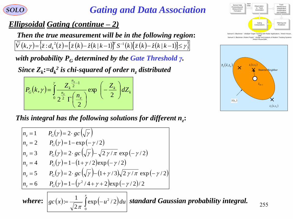
255
ktxz ,1
ktS
1|ˆ
kkz
ktxz ,2
ktxz ,3
Nearest-Neighbor
SOLO
Ellipsoidal Gating (continue – 2)
Then the true measurement will be in the following region:
with probability PG determined by the Gate Threshold γ.
Gating and Data Association
1|ˆ1|ˆ:,~ 12
kkzkzkSkkzkzzdzkVT
k
0 2
12
2exp
22
, kk
z
n
n
kG dZ
Z
n
ZkP
z
z
2/2/exp24/16
2/exp/23/125
2/exp2/114
2/exp/223
2/exp12
21
2
Gz
Gz
Gz
Gz
Gz
Gz
Pn
gcPn
Pn
gcPn
Pn
gcPn
This integral has the following solutions for different nz:
where: standard Gaussian probability integral.
x
duuxgc0
2 2/exp2
1:
Since Zk:=dk2 is chi-squared of order nz distributed
Sensor Data
Processing and
Measurement
Formation
Observation -
to - Track
Association
Input
DataTrack
Maintenance
) Initialization,
Confirmation
and Deletion(
Filtering and
Prediction
Gating
Computations
Samuel S . Blackman , " Multiple-Target Tracking with Radar Applications ", Artech House ,
1986Samuel S . Blackman , Robert Popoli , " Design and Analysis of Modern Tracking Systems
", Artech House , 1999
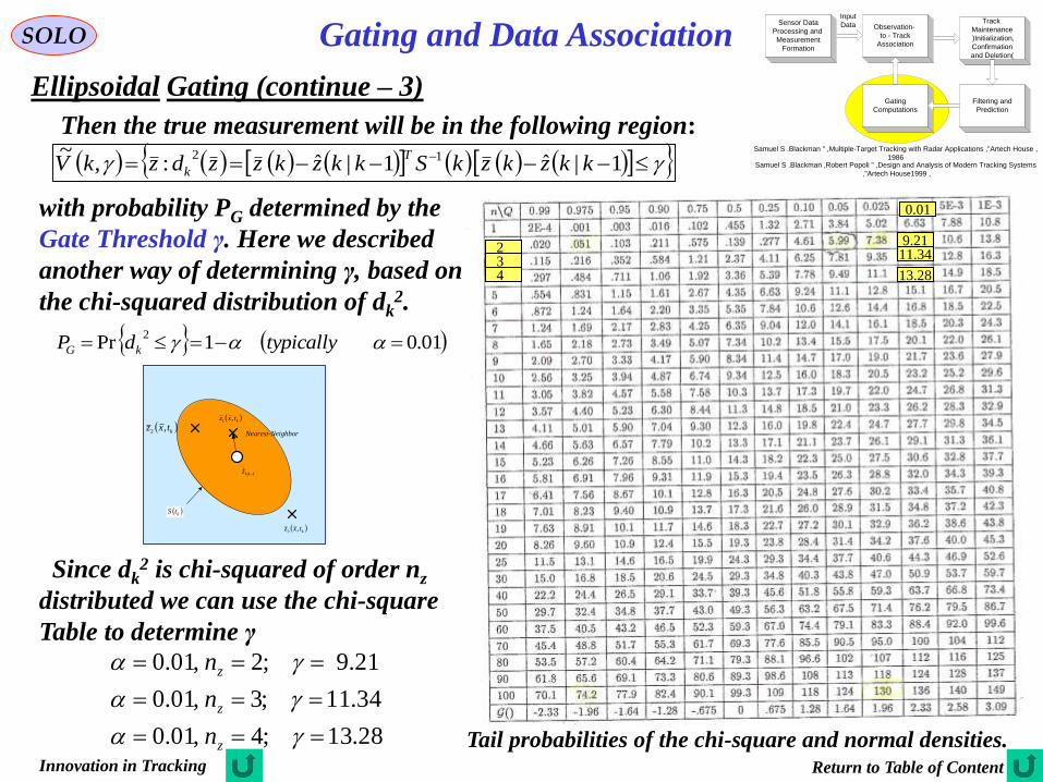
256
ktxz ,1
ktS
1|ˆ
kkz
ktxz ,2
ktxz ,3
Nearest-Neighbor
SOLO
Ellipsoidal Gating (continue – 3)
Then the true measurement will be in the following region:
with probability PG determined by the
Gate Threshold γ. Here we described
another way of determining γ, based on
the chi-squared distribution of dk2.
Gating and Data Association
Tail probabilities of the chi-square and normal densities.
9.2111.34
13.28
234
0.01
01.01Pr2
typicallydP kG
28.13;4,01.0
34.11;3,01.0
21.9;2,01.0
z
z
z
n
n
n
1|ˆ1|ˆ:,~ 12
kkzkzkSkkzkzzdzkVT
k
Since dk2 is chi-squared of order nz
distributed we can use the chi-square
Table to determine γ
Return to Table of ContentInnovation in Tracking
Sensor Data
Processing and
Measurement
Formation
Observation -
to - Track
Association
Input
DataTrack
Maintenance
) Initialization,
Confirmation
and Deletion(
Filtering and
Prediction
Gating
Computations
Samuel S . Blackman , " Multiple-Target Tracking with Radar Applications ", Artech House ,
1986Samuel S . Blackman , Robert Popoli , " Design and Analysis of Modern Tracking Systems
", Artech House , 1999
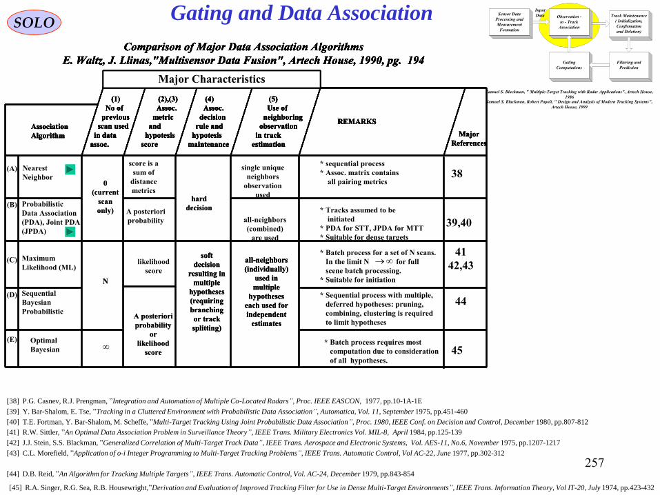
257
Gating and Data Association Sensor Data
Processing and
Measurement
Formation
Observation -
to - Track
Association
Input
Data Track Maintenance
( Initialization,
Confirmation
and Deletion)
Filtering and
Prediction
Gating
Computations
Samuel S. Blackman, " Multiple-Target Tracking with Radar Applications", Artech House,
1986Samuel S. Blackman, Robert Popoli, " Design and Analysis of Modern Tracking Systems",
Artech House, 1999
SOLO
Comparison of Major Data Association Algorithms
E. Waltz, J. Llinas,"Multisensor Data Fusion", Artech House, 1990, pg. 194
Major Characteristics
(1)
No of
previous
scan used
in data
assoc.
(2),(3)
Assoc.
metric
and
hypotesis
score
(4)
Assoc.
decision
rule and
hypotesis
maintenance
(5)
Use of
neighboring
observation
in track
estimation
Association
Algorithm
Nearest
Neighbor0
(current
scan
only)
score is a
sum of
distance
metricshard
decision
single unique
neighbors
observation
used
* sequential process
* Assoc. matrix contains
all pairing metrics
REMARKS
Major
References
38(A)
[38] P.G. Casnev, R.J. Prengman, ”Integration and Automation of Multiple Co-Located Radars”, Proc. IEEE EASCON, 1977, pp.10-1A-1E
[39] Y. Bar-Shalom, E. Tse, ”Tracking in a Cluttered Environment with Probabilistic Data Association”, Automatica, Vol. 11, September 1975, pp.451-460
[40] T.E. Fortman, Y. Bar-Shalom, M. Scheffe, ”Multi-Target Tracking Using Joint Probabilistic Data Association”, Proc. 1980, IEEE Conf. on Decision and Control, December 1980, pp.807-812
[41] R.W. Sittler, ”An Optimal Data Association Problem in Surveillance Theory”, IEEE Trans. Military Electronics Vol. MIL-8, April 1984, pp.125-139
[42] J.J. Stein, S.S. Blackman, ”Generalized Correlation of Multi-Target Track Data”, IEEE Trans. Aerospace and Electronic Systems, Vol. AES-11, No.6, November 1975, pp.1207-1217
[43] C.L. Morefield, ”Application of o-i Integer Programming to Multi-Target Tracking Problems”, IEEE Trans. Automatic Control, Vol AC-22, June 1977, pp.302-312
[44] D.B. Reid, ”An Algorithm for Tracking Multiple Targets”, IEEE Trans. Automatic Control, Vol. AC-24, December 1979, pp.843-854
[45] R.A. Singer, R.G. Sea, R.B. Housewright,”Derivation and Evaluation of Improved Tracking Filter for Use in Dense Multi-Target Environments”, IEEE Trans. Information Theory, Vol IT-20, July 1974, pp.423-432
Comparison of Major Data Association Algorithms
E. Waltz, J. Llinas,"Multisensor Data Fusion", Artech House, 1990, pg. 194
Major Characteristics
(1)
No of
previous
scan used
in data
assoc.
(2),(3)
Assoc.
metric
and
hypotesis
score
(4)
Assoc.
decision
rule and
hypotesis
maintenance
(5)
Use of
neighboring
observation
in track
estimation
Association
Algorithm
Probabilistic
Data Association
(PDA), Joint PDA
(JPDA)
0
(current
scan
only) A posteriori
probability
hard
decision
all-neighbors
(combined)
are used
* Tracks assumed to be
initiated
* PDA for STT, JPDA for MTT
* Suitable for dense targets
REMARKS
Major
References
39,40
(B)
Comparison of Major Data Association Algorithms
E. Waltz, J. Llinas,"Multisensor Data Fusion", Artech House, 1990, pg. 194
Major Characteristics
(1)
No of
previous
scan used
in data
assoc.
(2),(3)
Assoc.
metric
and
hypotesis
score
(4)
Assoc.
decision
rule and
hypotesis
maintenance
(5)
Use of
neighboring
observation
in track
estimation
Association
Algorithm
Maximum
Likelihood (ML)
N
likelihood
score
soft
decision
resulting in
multiple
hypotheses
(requiring
branching
or track
splitting)
all-neighbors
(individually)
used in
multiple
hypotheses
each used for
independent
estimates
* Batch process for a set of N scans.
In the limit N for full
scene batch processing.
* Suitable for initiation
REMARKS
Major
References
41
42,43(C)
Comparison of Major Data Association Algorithms
E. Waltz, J. Llinas,"Multisensor Data Fusion", Artech House, 1990, pg. 194
Major Characteristics
(1)
No of
previous
scan used
in data
assoc.
(2),(3)
Assoc.
metric
and
hypotesis
score
(4)
Assoc.
decision
rule and
hypotesis
maintenance
(5)
Use of
neighboring
observation
in track
estimation
Association
Algorithm
Sequential
Bayesian
Probabilistic
N
A posteriori
probability
or
likelihood
score
soft
decision
resulting in
multiple
hypotheses
(requiring
branching
or track
splitting)
all-neighbors
(individually)
used in
multiple
hypotheses
each used for
independent
estimates
* Sequential process with multiple,
deferred hypotheses: pruning,
combining, clustering is required
to limit hypotheses
REMARKS
Major
References
44(D)
Comparison of Major Data Association Algorithms
E. Waltz, J. Llinas,"Multisensor Data Fusion", Artech House, 1990, pg. 194
Major Characteristics
(1)
No of
previous
scan used
in data
assoc.
(2),(3)
Assoc.
metric
and
hypotesis
score
(4)
Assoc.
decision
rule and
hypotesis
maintenance
(5)
Use of
neighboring
observation
in track
estimation
Association
Algorithm
Optimal
Bayesian
A posteriori
probability
or
likelihood
score
soft
decision
resulting in
multiple
hypotheses
(requiring
branching
or track
splitting)
all-neighbors
(individually)
used in
multiple
hypotheses
each used for
independent
estimates
* Batch process requires most
computation due to consideration
of all hypotheses.
REMARKS
Major
References
45(E)

258
Sensor Data
Processing and
Measurement
Formation
Observation -
to - Track
Association
Input
Data Track Maintenance
( Initialization,
Confirmation
and Deletion)
Filtering and
Prediction
Gating
Computations
Samuel S. Blackman, " Multiple-Target Tracking with Radar Applications", Artech House,
1986Samuel S. Blackman, Robert Popoli, " Design and Analysis of Modern Tracking Systems",
Artech House, 1999
ktxz ,1
ktS
kk ttz |ˆ1
ktxz ,2
ktxz ,3
Nearest-Neighbor
SOLO
Nearest-Neighbor Standard Filter
In the Nearest-Neighbor Standard Filter (NNSF) the validated
measurement next to the predicted measurement is used for
updating the state of the target.
The distance measure to be minimizes is the weighted norm of
the innovation:
111|1ˆ1|1ˆ: 112 kikSkikkzzkSkkzzzdTT
where S is the covariance matrix of the innovation.
Gating and Data Association
The problem of choosing the Nearest-Neighbor is that with some
probability, is not the correct measurement. Therefore the NNSF
will sometimes use incorrect measurements while “believing”
that they are correct.
Gatting & Data Association Table

259
Sensor Data
Processing and
Measurement
Formation
Observation -
to - Track
Association
Input
Data Track Maintenance
( Initialization,
Confirmation
and Deletion)
Filtering and
Prediction
Gating
Computations
Samuel S. Blackman, " Multiple-Target Tracking with Radar Applications", Artech House,
1986Samuel S. Blackman, Robert Popoli, " Design and Analysis of Modern Tracking Systems",
Artech House, 1999
SOLO
Global Nearest-Neighbor (GNN) Algorithms
Gating and Data Association
Gatting & Data Association Table
• Several 2D Algorithms are available
- Hungarian Method (Kuhn)
- Munkres Algorithm
- JV, JVC (Jonker – Volgenant – Castanon) Algorithms
- Auction Algorithm (Bertsekas)
• All these algorithms give the EXACT global solution
• They are polynomial order of complexity
• Difference in the speed of computation
- Auction Algorithm is considered the best
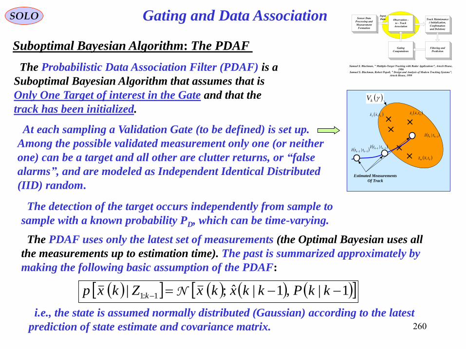
260
Sensor Data
Processing and
Measurement
Formation
Observation -
to - Track
Association
Input
Data Track Maintenance
( Initialization,
Confirmation
and Deletion)
Filtering and
Prediction
Gating
Computations
Samuel S. Blackman, " Multiple-Target Tracking with Radar Applications", Artech House,
1986Samuel S. Blackman, Robert Popoli, " Design and Analysis of Modern Tracking Systems",
Artech House, 1999
SOLO
Suboptimal Bayesian Algorithm: The PDAF
The Probabilistic Data Association Filter (PDAF) is a
Suboptimal Bayesian Algorithm that assumes that is
Only One Target of interest in the Gate and that the
track has been initialized.
At each sampling a Validation Gate (to be defined) is set up.
Among the possible validated measurement only one (or neither
one) can be a target and all other are clutter returns, or “false
alarms”, and are modeled as Independent Identical Distributed
(IID) random.
Gating and Data Association
The PDAF uses only the latest set of measurements (the Optimal Bayesian uses all
the measurements up to estimation time). The past is summarized approximately by
making the following basic assumption of the PDAF:
1|,1|ˆ;| 1:1 kkPkkxkxZkxp k N
i.e., the state is assumed normally distributed (Gaussian) according to the latest
prediction of state estimate and covariance matrix.
ktxz ,1
kV
1|ˆkk ttz
ktxz ,2
km txz ,
21 |ˆ kk ttz
32 |ˆ kk ttz
Estimated Measurements
Of Track
The detection of the target occurs independently from sample to
sample with a known probability PD, which can be time-varying.

261
Sensor Data
Processing and
Measurement
Formation
Observation -
to - Track
Association
Input
Data Track Maintenance
( Initialization,
Confirmation
and Deletion)
Filtering and
Prediction
Gating
Computations
Samuel S. Blackman, " Multiple-Target Tracking with Radar Applications", Artech House,
1986Samuel S. Blackman, Robert Popoli, " Design and Analysis of Modern Tracking Systems",
Artech House, 1999
ktxz ,1
kV
1|ˆkk ttz
ktxz ,2
km txz ,
SOLO
Suboptimal Bayesian Algorithm: The PDAF (continue – 1)
Following the white IID innovation assumption the Validation Gate
is defined by the ellipsoid
Gating and Data Association
ki
T
ki
k kkzkzkSkkzkzkzV 1|ˆ1|ˆ::~ 1
Tail probabilities of the chi-square and normal densities.
9.21
11.34
13.28
234
0.01
• From the chi-square table, given α and nz,
we can determine γ
28.13;4,01.0
34.11;3,01.0
21.9;2,01.0
z
z
z
n
n
n
The weighted norm innovation is chi-square
distributed with number of degrees of freedom
equal to dimension nz of the measurement.
The value of γ is determined by defining the
required probability PG that a measurement is
in the gate:
1~
: kG VkzPP
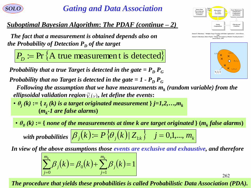
262
Sensor Data
Processing and
Measurement
Formation
Observation -
to - Track
Association
Input
Data Track Maintenance
( Initialization,
Confirmation
and Deletion)
Filtering and
Prediction
Gating
Computations
Samuel S. Blackman, " Multiple-Target Tracking with Radar Applications", Artech House,
1986Samuel S. Blackman, Robert Popoli, " Design and Analysis of Modern Tracking Systems",
Artech House, 1999
ktxz ,1
kV
1|ˆkk ttz
ktxz ,2
km txz ,
detectedistmeasurementrueAPr:DP
SOLO
Suboptimal Bayesian Algorithm: The PDAF (continue – 2)
The fact that a measurement is obtained depends also on
the Probability of Detection PD of the target
Gating and Data Association
Probability that a true Target is detected in the gate = PD PG
Probability that no Target is detected in the gate = 1 - PD PG
Following the assumption that we have measurements mk (random variable) from the
ellipsoidal validation region , let define the events: kV~
• θj (k) := { zj (k) is a target originated measurement } j=1,2,…,mk
(mk-1 are false alarms)
• θ0 (k) := { none of the measurements at time k are target originated } (mk false alarms)
with probabilities kkjj mjZkPk ,...,1,0|: :1
In view of the above assumptions those events are exclusive and exhaustive, and therefore
11
0
0
kk m
j
j
m
j
j kkk
The procedure that yields these probabilities is called Probabilistic Data Association (PDA).

263
Sensor Data
Processing and
Measurement
Formation
Observation -
to - Track
Association
Input
Data Track Maintenance
( Initialization,
Confirmation
and Deletion)
Filtering and
Prediction
Gating
Computations
Samuel S. Blackman, " Multiple-Target Tracking with Radar Applications", Artech House,
1986Samuel S. Blackman, Robert Popoli, " Design and Analysis of Modern Tracking Systems",
Artech House, 1999
SOLO
Suboptimal Bayesian Algorithm: The PDAF (continue – 3)
Gating and Data Association
βj (k) computation
kkkjkjj mjZmkZkPZkPk ,...,1,0,,||: 1:1:1
Z1:k - all measurements up to time k
Z (k) - all mk measurements at time k
Using Bayes’ rule for the mk exclusive and exhaustive events, we obtain:
km
i
kkikki
kkjkkj
kkjj mj
ZmkkZPZmkP
ZmkkZPZmkPZmkZkPk
k,...,1,0
,,|,|
,,|,|,,|
0
1:11:1
1:11:1
1:1
• θj (k) := { zj (k) is a target originated measurement } j=1,2,…,mk
(mk-1 are false alarms)
• θ0 (k) := { none of the measurements at time k are target originated} (mk false alarms)
ktxz ,1
kV
1|ˆkk ttz
ktxz ,2
km txz ,
Denoting by φ the number of false alarms (we have φ=mk-1 or φ=mk) we obtain:
0|
,...,1|1/1
0|1|10
,...,1|0|1/1
|,||1,1|
,|: 1
jmmP
mjmmPm
jmmPmmP
mjmmPmmPm
mmPmmkPmmPmmkP
ZmkPk
kk
kkkk
kkkk
kkkkkk
kkkkjkkkkj
k
kjj
1:1
0
1:11:1 ,|,,|,|
kk
m
i
kkikki ZmkZPZmkkZPZmkPk
Likelihood Function

264
Sensor Data
Processing and
Measurement
Formation
Observation -
to - Track
Association
Input
Data Track Maintenance
( Initialization,
Confirmation
and Deletion)
Filtering and
Prediction
Gating
Computations
Samuel S. Blackman, " Multiple-Target Tracking with Radar Applications", Artech House,
1986Samuel S. Blackman, Robert Popoli, " Design and Analysis of Modern Tracking Systems",
Artech House, 1999
SOLO
Suboptimal Bayesian Algorithm: The PDAF (continue – 4)
Gating and Data Association
km
i
kkikki
kkjkkj
kkjj mj
ZmkkZPZmkP
ZmkkZPZmkPZmkZkPk
k,...,1,0
,,|,|
,,|,|,,|
0
1:11:1
1:11:1
1:1
ktxz ,1
kV
1|ˆkk ttz
ktxz ,2
km txz ,
Denoting by φ the number of false alarms (we have φ=mk-1 or φ=mk) we obtain:
0|
,...,1|1/1,|: 1:1
jmmP
mjmmPmZmkPk
kk
kkkk
kkjj
βj (k) computation (continue – 1)
Using Bayes Formula we obtain:
k
kGD
k
m
k
PP
kkkk
mP
mPP
mP
mPmmPmmP
kGD
111||1
1
k
kGD
k
m
k
PP
kkkk
mP
mPP
mP
mPmmPmmP
kGD
1||
1
where μF is the probability mass function (pmf) of the number of false alarms and PD PG is the
probability that the target has been detected and its measurements fell in the gate.
The common denominator is: kGDkGDk mPPmPPmP 11

265
Sensor Data
Processing and
Measurement
Formation
Observation -
to - Track
Association
Input
Data Track Maintenance
( Initialization,
Confirmation
and Deletion)
Filtering and
Prediction
Gating
Computations
Samuel S. Blackman, " Multiple-Target Tracking with Radar Applications", Artech House,
1986Samuel S. Blackman, Robert Popoli, " Design and Analysis of Modern Tracking Systems",
Artech House, 1999
ktxz ,1
kV
1|ˆkk ttz
ktxz ,2
km txz ,
SOLO
Suboptimal Bayesian Algorithm: The PDAF (continue – 5)
Gating and Data Association
km
i
kkikki
kkjkkj
kkjj mj
ZmkkZPZmkP
ZmkkZPZmkPZmkZkPk
k,...,1,0
,,|,|
,,|,|,,|
0
1:11:1
1:11:1
1:1
We obtained:
01/11/1
,...,11/1/1,|:
1
1
1:1
jmmPPPPmmPP
mjmmPPPPPPmZmkPk
kFkFGDGDkFkFGD
kkFkFGDGDGDk
kkjj
βj (k) computation (continue – 2)
Two methods can be used to compute μF (the pmf of false alarms):
(i) A Poisson model with a certain spatial density λ
(parametric):
!k
m
V
kFm
Vem
k
(ii) A (nonparametric) diffuse prior model: 1kFkF mm
011
,...,11,|:
1
1
1:1
jkVPPmPPkVPP
mjkVPPmPPPPZmkPk
GDkGDGD
kGDkGDGD
kkjj
01
,...,1/,|: 1:1
jPP
mjmPPZmkPk
GD
kkGD
kkjj
The nonparametric model can be obtained from Poisson model by choosing: kVmk /:
V (k) volume of the
Ellipsoid Gate
2/12/2
12
, kSn
kV z
z
n
z
n

266
Sensor Data
Processing and
Measurement
Formation
Observation -
to - Track
Association
Input
Data Track Maintenance
( Initialization,
Confirmation
and Deletion)
Filtering and
Prediction
Gating
Computations
Samuel S. Blackman, " Multiple-Target Tracking with Radar Applications", Artech House,
1986Samuel S. Blackman, Robert Popoli, " Design and Analysis of Modern Tracking Systems",
Artech House, 1999
ktxz ,1
kV
1|ˆkk ttz
ktxz ,2
km txz ,
SOLO
Suboptimal Bayesian Algorithm: The PDAF (continue – 6)
Gating and Data Association
km
i
kkikki
kkjkkj
kkjj mj
ZmkkZPZmkP
ZmkkZPZmkPZmkZkPk
k,...,1,0
,,|,|
,,|,|,,|
0
1:11:1
1:11:1
1:1
Let compute:
βj (k) computation (continue – 3)
V (k) volume of the
Ellipsoid Gate
2/12/2
12
, kSn
kV z
z
n
z
n
Since for mk measurements we can have only one target and mk-1 false alarms or
mk false alarms, we obtain
k
k
m
j
kkji
tindependen
tsmeasuremenkkjmkkj ZmkzPZmkzzPZmkkZP
1
1:11:111:1 ,,|,,|,,,,|
Assumptions: Gaussian pdf of correct target in the ellipsoidal gate,
with probability PG and uniform distribution of false alarms inside V (k).
TargetTrue2
2/exp,0;
TargetNew1
,,| 11:1
kS
kikSkiPkSkiP
orAlarmFalseistmeasuremeniifV
ZmkzPj
T
j
GjG
kkjj
1-1-
N
0
,,1,0;,,|,,|
11
1
1:1
1
jkV
mjkSkiPkVZmkzPZmkkZP
k
kk
m
kjG
mm
j
kkjj
k
kj
N
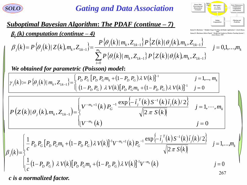
267
Sensor Data
Processing and
Measurement
Formation
Observation -
to - Track
Association
Input
Data Track Maintenance
( Initialization,
Confirmation
and Deletion)
Filtering and
Prediction
Gating
Computations
Samuel S. Blackman, " Multiple-Target Tracking with Radar Applications", Artech House,
1986Samuel S. Blackman, Robert Popoli, " Design and Analysis of Modern Tracking Systems",
Artech House, 1999
SOLO
Suboptimal Bayesian Algorithm: The PDAF (continue – 7)
Gating and Data Association
km
i
kkikki
kkjkkj
kkjj mj
ZmkkZPZmkP
ZmkkZPZmkPZmkZkPk
k,...,1,0
,,|,|
,,|,|,,|
0
1:11:1
1:11:1
1:1
βi (k) computation (continue – 4)
We obtained for parametric (Poisson) model:
0
,,12
2/exp
,,|
1
11
1:1
jkV
mjkS
kikSkiPkV
ZmkkZP
k
k
m
k
j
T
j
G
m
kkj
011
,...,11,|:
1
1
1:1
jkVPPmPPkVPP
mjkVPPmPPPPZmkPk
GDkGDGD
kGDkGDGD
kkjj
0111
,...,12
2/exp1
1
1
1
111
jkVkVPPmPPkVPPc
mjkS
kikSkiPkVkVPPmPPPP
ck
k
k
m
GDkGDGD
k
j
T
j
G
m
GDkGDGD
j
c is a normalized factor.
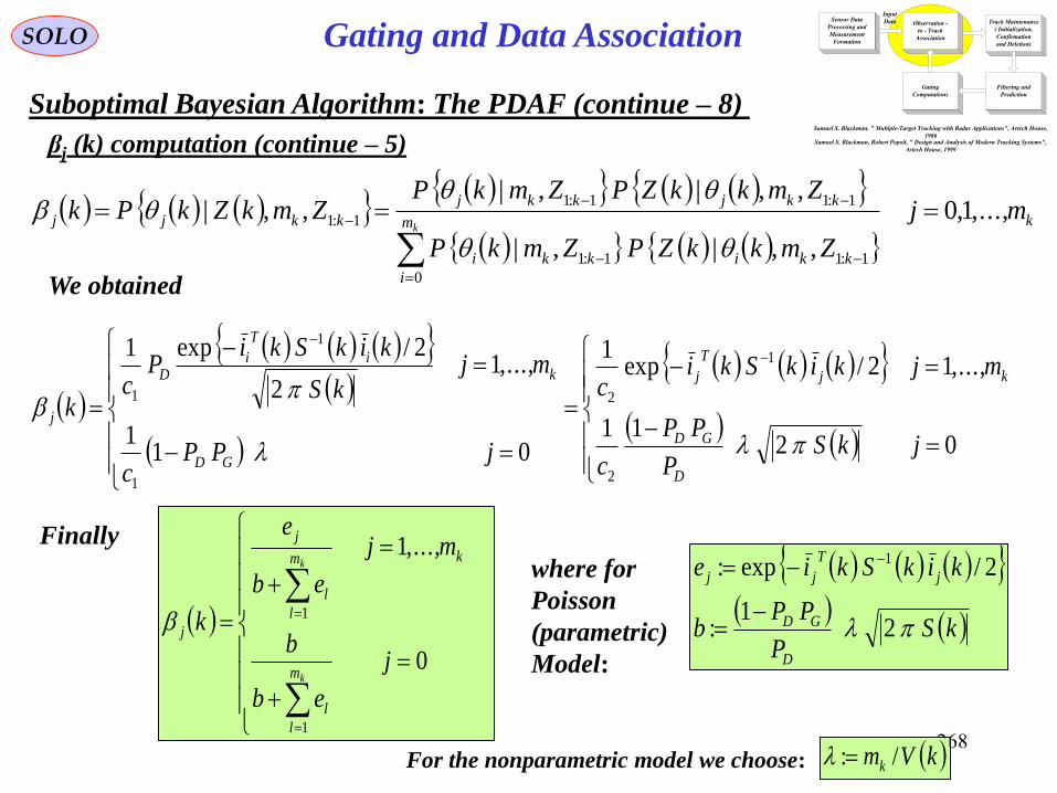
268
Sensor Data
Processing and
Measurement
Formation
Observation -
to - Track
Association
Input
Data Track Maintenance
( Initialization,
Confirmation
and Deletion)
Filtering and
Prediction
Gating
Computations
Samuel S. Blackman, " Multiple-Target Tracking with Radar Applications", Artech House,
1986Samuel S. Blackman, Robert Popoli, " Design and Analysis of Modern Tracking Systems",
Artech House, 1999
SOLO
Suboptimal Bayesian Algorithm: The PDAF (continue – 8)
Gating and Data Association
km
i
kkikki
kkjkkj
kkjj mj
ZmkkZPZmkP
ZmkkZPZmkPZmkZkPk
k,...,1,0
,,|,|
,,|,|,,|
0
1:11:1
1:11:1
1:1
βj (k) computation (continue – 5)
We obtained
0211
,...,12/exp1
011
,...,12
2/exp1
2
1
2
1
1
1
jkSP
PP
c
mjkikSkic
jPPc
mjkS
kikSkiP
ck
D
GD
kj
T
j
GD
ki
T
iD
j
Finally
0
,...,1
1
1
j
eb
b
mj
eb
e
k
k
k
m
l
l
km
l
l
j
j
kSP
PPb
kikSkie
D
GD
j
T
jj
21
:
2/exp: 1
where for
Poisson
(parametric)
Model:
For the nonparametric model we choose: kVmk /:
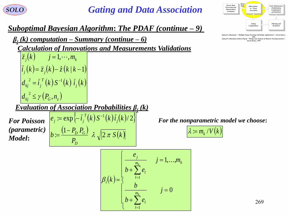
269
Sensor Data
Processing and
Measurement
Formation
Observation -
to - Track
Association
Input
Data Track Maintenance
( Initialization,
Confirmation
and Deletion)
Filtering and
Prediction
Gating
Computations
Samuel S. Blackman, " Multiple-Target Tracking with Radar Applications", Artech House,
1986Samuel S. Blackman, Robert Popoli, " Design and Analysis of Modern Tracking Systems",
Artech House, 1999
SOLO
Suboptimal Bayesian Algorithm: The PDAF (continue – 9)
Gating and Data Association
βj (k) computation – Summary (continue – 6)
Evaluation of Association Probabilities βj (k)
0
,...,1
1
1
j
eb
b
mj
eb
e
k
k
k
m
l
l
km
l
l
j
i
kSP
PPb
kikSkie
D
GD
j
T
jj
21
:
2/exp: 1
For Poisson
(parametric)
Model:
For the nonparametric model we choose:
kVmk /:
Calculation of Innovations and Measurements Validations
zGkj
j
T
jkj
jj
kj
nPd
kikSkid
kkzkzki
mjkz
,
1|ˆ
,,1
2
12
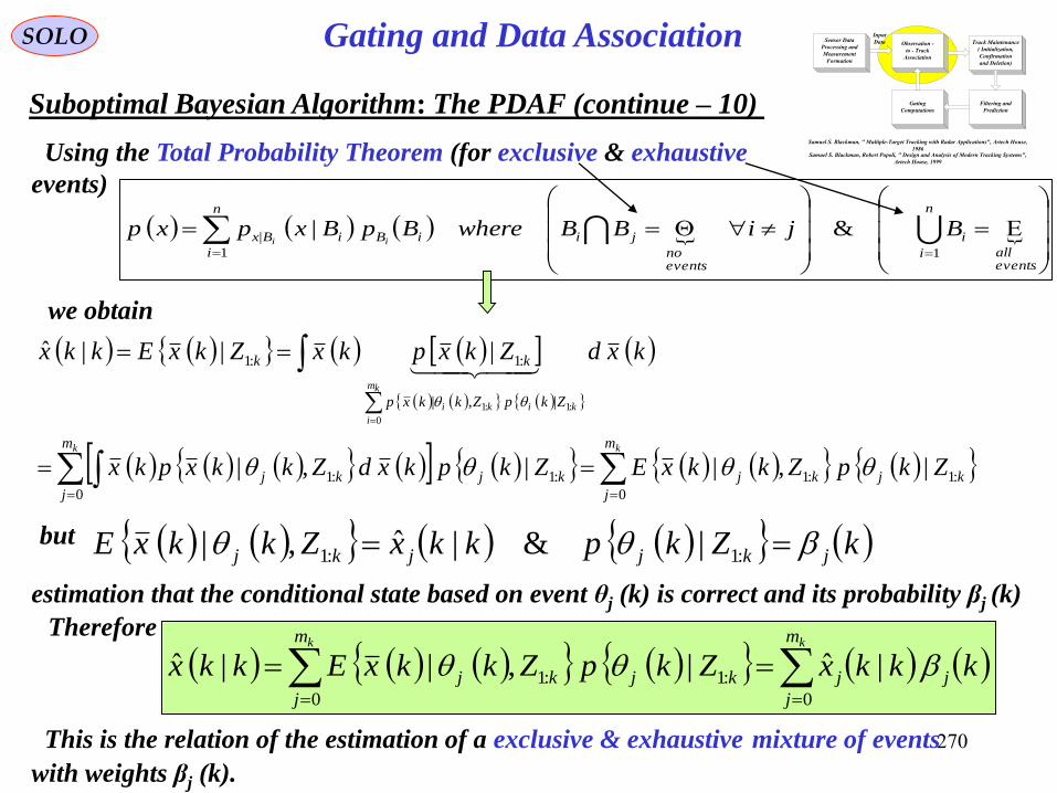
270
Sensor Data
Processing and
Measurement
Formation
Observation -
to - Track
Association
Input
Data Track Maintenance
( Initialization,
Confirmation
and Deletion)
Filtering and
Prediction
Gating
Computations
Samuel S. Blackman, " Multiple-Target Tracking with Radar Applications", Artech House,
1986Samuel S. Blackman, Robert Popoli, " Design and Analysis of Modern Tracking Systems",
Artech House, 1999
SOLO
Suboptimal Bayesian Algorithm: The PDAF (continue – 10)
Using the Total Probability Theorem (for exclusive & exhaustive
events)
Gating and Data Association
eventsall
n
i
i
eventsno
ji
n
i
iBiBx BjiBBwhereBpBxpxpii
11
| &|
we obtain
kk
km
i
kiki
m
j
kjkj
m
j
kjkj
ZkpZkkxp
kk
ZkpZkkxEZkpkxdZkkxpkx
kxdZkxpkxZkxEkkx
0
:1:1
0
:1:1
|,|
:1:1
|,||,|
|||ˆ
0
:1:1
but kZkpkkxZkkxE jkjjkj :1:1 |&|ˆ,|
Therefore
kk m
j
jj
m
j
kjkj kkkxZkpZkkxEkkx00
:1:1 |ˆ|,||ˆ
estimation that the conditional state based on event θj (k) is correct and its probability βj (k)
This is the relation of the estimation of a exclusive & exhaustive mixture of events
with weights βj (k).

271
Sensor Data
Processing and
Measurement
Formation
Observation -
to - Track
Association
Input
Data Track Maintenance
( Initialization,
Confirmation
and Deletion)
Filtering and
Prediction
Gating
Computations
Samuel S. Blackman, " Multiple-Target Tracking with Radar Applications", Artech House,
1986Samuel S. Blackman, Robert Popoli, " Design and Analysis of Modern Tracking Systems",
Artech House, 1999
SOLO
Suboptimal Bayesian Algorithm: The PDAF (continue – 11)
Gating and Data Association
It is given by the Kalman Filter topology:
kkx j |ˆ is the update state estimation conditioned on event θj (k) is correct.
11|11
1|ˆ1|ˆ1|ˆ|ˆ
1
kSkHkkPkK
kkzkzkKkkxkikKkkxkkx
T
jjj
For j = 1,…,mk (a possible target detected in the Validation Gate)
1|ˆ|ˆ0 kkxkkx
Therefore
kikKkkxkkikKkkkx
kkikKkkxkkkxkkx
ki
m
j
jj
m
j
j
m
j
jj
m
j
jj
kk
kk
1|ˆ1|ˆ
1|ˆ|ˆ|ˆ
0
1
0
00
For i = 0 (no target detected in the Validation Gate) the innovation is 0|0 kki
kikKkkxkkx 1|ˆ|ˆ
where is the combined innovation.
km
j
jj kkiki0
:

272
Sensor Data
Processing and
Measurement
Formation
Observation -
to - Track
Association
Input
Data Track Maintenance
( Initialization,
Confirmation
and Deletion)
Filtering and
Prediction
Gating
Computations
Samuel S. Blackman, " Multiple-Target Tracking with Radar Applications", Artech House,
1986Samuel S. Blackman, Robert Popoli, " Design and Analysis of Modern Tracking Systems",
Artech House, 1999
km
j
jkj
Tof
Mixture
eventsexhaustiveexclusive
k
T
kZkkkxkxkkxkxE
ZkkxkxkkxkxEkkP
0
:1&
:1
,||ˆ|ˆ
||ˆ|ˆ|
kk m
j
jj
m
j
kjkj kkkxZkpZkkxEkkx00
:1:1 |ˆ|,||ˆ
SOLO
Suboptimal Bayesian Algorithm: The PDAF (continue – 12)
Gating and Data Association
The covariance of the mixture is given by
km
j
j
T
jjjj kkkxkkxkkxkxkkxkkxkkxkxE0
|ˆ|ˆ|ˆ|ˆ|ˆ|ˆ
kk
j
m
j
T
ijj
m
j
j
kkP
jj kkxkkxkkkxkxEkkkxkxkkxkxE0
00
|
|ˆ|ˆ|ˆ|ˆ|ˆ
k km
j
m
j
j
T
jjj
T
jj kkkxkkxkkxkkxkkkxkxEkkxkkx0 0
0
|ˆ|ˆ|ˆ|ˆ|ˆ|ˆ|ˆ
kk m
j
j
T
jj
m
j
jj kkkxkkxkkxkkxkkkPkkP00
|ˆ|ˆ|ˆ|ˆ||
1||0 kkPkkP No target in Validated Gate
k
T
j mjkKkSkKkkPkkP ,,11|| 1 One target in Validated Gate

273
Sensor Data
Processing and
Measurement
Formation
Observation -
to - Track
Association
Input
Data Track Maintenance
( Initialization,
Confirmation
and Deletion)
Filtering and
Prediction
Gating
Computations
Samuel S. Blackman, " Multiple-Target Tracking with Radar Applications", Artech House,
1986Samuel S. Blackman, Robert Popoli, " Design and Analysis of Modern Tracking Systems",
Artech House, 1999
SOLO
Suboptimal Bayesian Algorithm: The PDAF (continue – 13)
Gating and Data Association
kk m
j
j
T
jj
m
j
jj kkkxkkxkkxkkxkkkPkkP00
|ˆ|ˆ|ˆ|ˆ||
k
Tc
j mjkKkSkKkkPkkPkkP ,,11||| 1
Since
kkkkk m
j
j
m
j
j 0
10
11
and
kPd
m
j
j
T
jj
ck
kkkxkkxkkxkkxkkPkkkPkkkP
0
00 |ˆ|ˆ|ˆ|ˆ|11||
1||0 kkPkkP
We have:
kkxkkxkkkxkkxkkkxkkxkkkxkkx
kkxkkkxkkkxkkxkkkxkkxkkxkkx
Tm
j
j
T
jj
m
j
j
T
kkx
m
j
j
T
j
T
kkx
m
j
jj
m
j
j
T
jj
m
j
j
T
jj
kk
T
k
kkk
|ˆ|ˆ|ˆ|ˆ|ˆ|ˆ|ˆ|ˆ
|ˆ|ˆ|ˆ|ˆ|ˆ|ˆ|ˆ|ˆ
0
1
0
|ˆ
0
|ˆ
000
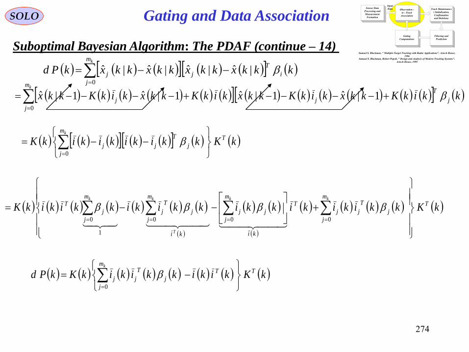
274
Sensor Data
Processing and
Measurement
Formation
Observation -
to - Track
Association
Input
Data Track Maintenance
( Initialization,
Confirmation
and Deletion)
Filtering and
Prediction
Gating
Computations
Samuel S. Blackman, " Multiple-Target Tracking with Radar Applications", Artech House,
1986Samuel S. Blackman, Robert Popoli, " Design and Analysis of Modern Tracking Systems",
Artech House, 1999
SOLO
Suboptimal Bayesian Algorithm: The PDAF (continue – 14)
Gating and Data Association
km
j
i
T
jj kkkxkkxkkxkkxkPd0
|ˆ|ˆ|ˆ|ˆ
km
j
j
T
jj kkikKkkxkikKkkxkikKkkxkikKkkx0
1|ˆ1|ˆ1|ˆ1|ˆ
kKkkikikikikK Tm
j
j
T
jj
k
0
kKkkikikikkikkikikkikikK Tm
j
j
T
jj
T
ki
m
j
jj
ki
m
j
j
T
j
m
j
j
Tkk
T
kk
000
1
0
kKkikikkikikKkPd TTm
j
j
T
jj
k
0

275
Sensor Data
Processing and
Measurement
Formation
Observation -
to - Track
Association
Input
Data Track Maintenance
( Initialization,
Confirmation
and Deletion)
Filtering and
Prediction
Gating
Computations
Samuel S. Blackman, " Multiple-Target Tracking with Radar Applications", Artech House,
1986Samuel S. Blackman, Robert Popoli, " Design and Analysis of Modern Tracking Systems",
Artech House, 1999
SOLO
Suboptimal Bayesian Algorithm: The PDAF (continue – 15)
Gating and Data Association
kPdkkPkkkPkkkP c |11|| 00
kKkikikkikikKkPd TTm
j
j
T
jj
k
0
:
kKkSkKkkPkkP Tc 11||
Finally we obtained

276
SOLO
1|1 kkP
State CovarianceState Estimation
Predicted State
1|111| kkxkFkkx
kRkHkkPkHkS T 1|
Innovation Covariance
111|111| kQkFkkPkFkkP T
Covariance of Predicted State
kSkHkkPkK T 11|
Filter Gain
kKkikikikikKkPd TTm
j
T
jjj
k
1
Effect of Measurement Origin
on State Covarriance
Update State Covariance
kPdkkPkHkKI
kkPkkP
1|1
1||
0
0
Combined Innovation
km
j
jj kiki1
Update State Estimation
kikKkkxkkx 1||
kS
ki j
j
ki
kz j
One Cycle of
PDAF
Measurements
1|1 kkx
k
m
l
lj
m
l
l
j
kjDj
n
GD
mjebe
nobservatiovalidNojebb
mjdPe
SPPb
k
k
z
1/
0/
,,2,12/exp
21
1
1
2
2/
Evaluation of Association Probabilities
Predicted Measurements
1|1|ˆ kkxkHkkz
zGkj
j
T
jkj
jj
kj
nPd
kikSkid
kkzkzki
mjkz
,
1|ˆ
,,2,1
2
12
Calculation of Innovation and
Measurement Validation
Suboptimal Bayesian Algorithm: The PDAF (continue – 16)
Gating and Data Association

277
Sensor Data
Processing and
Measurement
Formation
Observation -
to - Track
Association
Input
DataTrack
Maintenance
(Initialization,
Confirmation
and Deletion)
Filtering and
Prediction
Gating
Computations
Samuel S . Blackman , " Multiple-Target Tracking with Radar Applications ", Artech House ,
1986Samuel S . Blackman , Robert Popoli , " Design and Analysis of Modern Tracking Systems
", Artech House , 1999
SOLO
Track Initialization, Maintenance & Deletion
Track Life Cycle
(Initialization, Maintenance & Deletion)
Initial/
Terminal
State
Preliminary
Track
Tentative
Track
Confirmed
Track
No. of
Detections
≥ M
No
Second
Detection
Wait N
Scans
Initial
Detection
No. of
Detections
< M
L
Consecutive
Missed
Detections
No
Detection
No L
Consecutive
Missed
Detections

278
Sensor Data
Processing and
Measurement
Formation
Observation -
to - Track
Association
Input
DataTrack
Maintenance
(Initialization,
Confirmation
and Deletion)
Filtering and
Prediction
Gating
Computations
Samuel S . Blackman , " Multiple-Target Tracking with Radar Applications ", Artech House ,
1986Samuel S . Blackman , Robert Popoli , " Design and Analysis of Modern Tracking Systems
", Artech House , 1999
SOLO
Track Initialization
Track Life Cycle
(Initialization, Maintenance & Deletion)
Every Detection unassociated to an existing Track may be a False Alarm or a New Target.
A Track Formation requires a Measurement-to-Measurement Association.
Logic to Track Initialization (2 Detections for a Preliminary Track followed by
M detections out of N scans):
Every Unassociated Detection is a “Track Initiator”, yields a “Tentative Track”. 1
Around the Initial Detection a Gate is set up based on2
• assumed maximum and minimum Target motion parameters.
• the measured noise intensities.
If is a Target, that gave rise to the initiator in the first scan, if detected in the second scan
will fall in the Gate with nearly unity probability. Following a detection, in the second scan,
this Track becomes a Preliminary Track, if there is no detection, this Track is dropped.
Since the Preliminary Track has two measurements, a Kalman Filter can be initialized and
used to set up a Gate for the next (third) sampling time.
3
Starting from the third scan a logic of M detections out of N scans (frames) is used for the
subsequent Gates.
4
If at the end (scan N + 2 at the latest) the logic requirement is satisfied, the Track becomes a
Confirmed Track, otherwise is dropped.
5

279
Sensor Data
Processing and
Measurement
Formation
Observation -
to - Track
Association
Input
DataTrack
Maintenance
(Initialization,
Confirmation
and Deletion)
Filtering and
Prediction
Gating
Computations
Samuel S . Blackman , " Multiple-Target Tracking with Radar Applications ", Artech House ,
1986Samuel S . Blackman , Robert Popoli , " Design and Analysis of Modern Tracking Systems
", Artech House , 1999
SOLO
Track Initialization
Track Maintenance
(Initialization, Maintenance & Deletion)
Target Model
• Target System is given by:
kkkk
kkkkkkk
vxHz
wuGxx
111111
kv
kH kzkx
kx1 k
1kw1k
1kx
1ku 1kG
1zDelay
• Target Filter Model is given by:
1|1|
111|111|
ˆˆ
ˆˆ
kkkkk
kkkkkkk
xHz
uGxx
• Filter Initialization is done in two steps:
1. Following an unassociated detection a Preliminary Large Gate is defined
2. After a second detection is associated in the Preliminary Gate the Kalman
Filter is initiated using the two measurements by defining
A Preliminary New Track is established. 0|00|0 ,ˆ Px

280
Sensor Data
Processing and
Measurement
Formation
Observation -
to - Track
Association
Input
DataTrack
Maintenance
(Initialization,
Confirmation
and Deletion)
Filtering and
Prediction
Gating
Computations
Samuel S . Blackman , " Multiple-Target Tracking with Radar Applications ", Artech House ,
1986Samuel S . Blackman , Robert Popoli , " Design and Analysis of Modern Tracking Systems
", Artech House , 1999
SOLO
Track Initialization
Track Life Cycle
(Initialization, Maintenance & Deletion)
Track # 1Track # 2
New Targets
or
False Alarms
Old Targets
Scan # m
Scan # m+1
Scan # m+2
Scan # m+3
Tgt
# 1
Tgt
# 2
Tgt
# 1
Tgt
# 1
Tgt
# 2
Tgt
# 2
Tgt
# 2
Preliminary
Track # 1
Preliminary
Track # 2False
Alarm
False
Alarm
Tgt
# 3

281
Sensor Data
Processing and
Measurement
Formation
Observation -
to - Track
Association
Input
DataTrack
Maintenance
(Initialization,
Confirmation
and Deletion)
Filtering and
Prediction
Gating
Computations
Samuel S . Blackman , " Multiple-Target Tracking with Radar Applications ", Artech House ,
1986Samuel S . Blackman , Robert Popoli , " Design and Analysis of Modern Tracking Systems
", Artech House , 1999
SOLO
Track Initialization
Track Life Cycle
(Initialization, Maintenance & Deletion)
Target Model (continue – 1)
• If detection (probability PD ) can be associated to the track, i.e. is in the
Acceptance Gate (probability PG ): 1|1|ˆˆ
kkkk
T
kkk zzSzz
• At each scan we perform State and Innovation Covariance Prediction:
k
T
kkkkk
k
T
kkkkkk
RHPHS
QPP
1|
111|111|
we update the Detection Indicator Vector:
otherwise
katgatetheindetectionaisifk
0
1
and the State and State Covariance are updated, accordingly
kkkkkkkk
kkkkkkkkk
k
T
kkkk
KSKPP
zzKxx
SHPK
1||
1|1||
1
1|
ˆˆˆ
• If in M scans out of N we have an associated to Track detection the Track is Confirmed
otherwise is dropped.

282
Sensor Data
Processing and
Measurement
Formation
Observation -
to - Track
Association
Input
DataTrack
Maintenance
(Initialization,
Confirmation
and Deletion)
Filtering and
Prediction
Gating
Computations
Samuel S . Blackman , " Multiple-Target Tracking with Radar Applications ", Artech House ,
1986Samuel S . Blackman , Robert Popoli , " Design and Analysis of Modern Tracking Systems
", Artech House , 1999
State Detection Sequence
Indicator Vector
δ = 0 No Detection
δ = 1 Detection
Transition
D = detection
A = Acceptance
1 Initial (zero state)
2 δ2 = [1]
3 δ3 = [1 1]
4 δ4= [1 1 1]
5 δ5= [1 1 1 0]
6 δ6 = [1 1 0]
7 δ7= [1 1 0 1]
8a δ8a = [1 1 1 1] Confirmed State
8b δ3 = [1 1 1 0 1] Confirmed State
8c δ3 = [1 1 0 1 1] Confirmed State
1;2 DD
SOLO
Track Initialization
Track Life Cycle
(Initialization, Maintenance & Deletion)
Markov Chain for the Track Initialization Process for M=2, N=3
1;3 DD
6;4 AA
5;8 AaA
1;8 AbA
1;7 AA
1;8 AcA
DD
1 2 3 4
5
6 7
8a
8b
8c
D A
D
D 1
12 113 1114
01115
0116 10117
Preliminary
Track
Track
Confirmation
m=2/n=3
Initial
State
D
A A
A
AA
A A
A
A
State i of the Markov Chain is defined by the Detection Sequence Indicator Vector δi, where, for
example, δ7=[1 1 0 1] means Detection (D), followed by Detection (A), No Detection ( ), Detection (A).A
The Markov Chain probability vector, denoted by
μ (k), has components:
μi (k)= Pr { the chain is in State i at time k }
From the Markov Chain description by the Table or by the Graph we can define the relation:
000,10:..,1,01 821 CIkkk

284
Sensor Data
Processing and
Measurement
Formation
Observation -
to - Track
Association
Input
DataTrack
Maintenance
(Initialization,
Confirmation
and Deletion)
Filtering and
Prediction
Gating
Computations
Samuel S . Blackman , " Multiple-Target Tracking with Radar Applications ", Artech House ,
1986Samuel S . Blackman , Robert Popoli , " Design and Analysis of Modern Tracking Systems
", Artech House , 1999
\ 1 2 3 4 5 6 7 8
1 1-πD πD 0 0 0 0 0 0
2 1-πD 0 πD 0 0 0 0 0
3 0 0 0 πA 0 1-πA 0 0
4 0 0 0 0 1-πA 0 0 πA
5 1-πA 0 0 0 0 0 0 πA
6 1-πA 0 0 0 0 0 0 πA
7 1-πA 0 0 0 0 πA 0 0
8 0 0 0 0 0 0 0 1
SOLO
Track Initialization
Track Life Cycle
(Initialization, Maintenance & Deletion)
Markov Chain for the Track Initialization Process for M=2, N=3 (continue – 2)
The acceptance probability is πA = PD• PG
where PD = Probability of Detection
PG = Probability that the true measurement will fall in the Gate
000,10:..,1,01 821 CIkkk
Π
1 2 3 4
5
6 7
8a
8b
8c
D A
D
D 1
12 113 1114
01115
0116 10117
Preliminary
Track
Track
Confirmation
m=2/n=3
Initial
State
D
A A
A
AA
A
A
A
A
Since for each state we can move to only two states with probabilities πD /πA and 1 – πD /1- πA the
coefficients of Π matrix must satisfy:1
j
ji
The initialization probability is πD

285
Sensor Data
Processing and
Measurement
Formation
Observation -
to - Track
Association
Input
DataTrack
Maintenance
(Initialization,
Confirmation
and Deletion)
Filtering and
Prediction
Gating
Computations
Samuel S . Blackman , " Multiple-Target Tracking with Radar Applications ", Artech House ,
1986Samuel S . Blackman , Robert Popoli , " Design and Analysis of Modern Tracking Systems
", Artech House , 1999
SOLO
Track Initialization
Track Life Cycle
(Initialization, Maintenance & Deletion)
Markov Chain for the Track Initialization Process for M=2, N=3 (continue – 2)
000,10:..,1,01 821 CIkkk
1 2 3 4
5
6 7
8a
8b
8c
D A
D
D 1
12 113 1114
01115
0116 10117
Preliminary
Track
Track
Confirmation
m=2/n=3
Initial
State
D
A A
A
AA
A
A
A
A
and:
The Track Confirmation is attained in State 8.
Therefore:
k8
Ckk 188 kk
Ck k
C
C
kk
kkk
1
08
C
C
kk
kkkk
1
0188
The Average Confirmation Time of a Target-originated Sequence is:
C
k
C kkkkt
1
88 1

286
Target Estimators
Filters for Maneuvering Target Detection
• Maneuver Detection Scheme
• Hybrid State Estimation Techniques
- Jump Markov Linear System (JMLS)
- Interactive Multiple Model (IMM)
- Variable Structure IMM
• Cramér - Rao Lower Bound (CRLB) for JMLS
SOLO

287
Target Estimators
Filters for Maneuvering Target Detection – Background
• The motion of a real target never follows the same dynamic model all the time.
• Essentially, there are (long – relative to measurement updates) period of constant
velocity (CV) motion with sudden changes in speed and heading.
• The measurements are of target position and velocity (sometimes), but not target
acceleration.
• There are two main approaches to deal with maneuvering targets using the
Kalman Filter framework:
SOLO
- Maneuver Detection Basic Schemes
- Hybrid-state estimation techniques, where a few predefined target maneuver
models run in parallel, using the same measurements, and recursively we
check what is the most plausible model in each time interval.
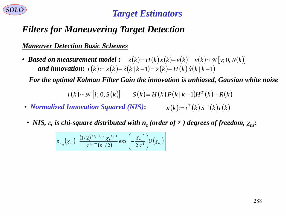
288
Target Estimators
Filters for Maneuvering Target Detection
SOLO
Maneuver Detection Basic Schemes
kRkHkkPkHkSkSiki T 1|,0;~ N
• Normalized Innovation Squared (NIS): kikSkik T 1:
For the optimal Kalman Filter Gain the innovation is unbiased, Gausian white noise
1|ˆ1|ˆ: kkxkHkzkkzkzkiand innovation:
• Based on measurement model : kRvkvkvkxkHkz ,0;~N
• NIS, ε, is chi-square distributed with nz (order of ) degrees of freedom, χnz:z
z
z
z
zz
zzn n
n
z
n
n
k
n
n Un
p
2
212/2
2exp
2/
2/1

289
SOLO
Tail probabilities of the chi-square and normal densities.
9.2111.34
13.28
234
• From the chi-square table
we can determine εmax
28.13;4,01.0
34.11;3,01.0
21.9;2,01.0
max
max
max
z
z
z
n
n
n
• For non-maneuvering motion
01.01Pr max typicallyk
Target Estimators
Filters for Maneuvering Target Detection
Maneuver Detection Basic Schemes (continue – 1)
0.01
122 , ktxz
12 ktS
kk ttz |ˆ12
max kTarget Maneuvers
1
111 , ktxz
11 ktS
kk ttz |ˆ11
max kNon-maneuvering
Target
• Once a maneuver is detected Target
dynamic model must be changed.
• In the same way we can detect the
end of a Target maneuver.

290
SOLO Target Estimators
Filters for Maneuvering Target Detection
Maneuver Detection Basic Schemes (continue – 2)
Return to Table of Content

291
SOLO Target EstimatorsThe Hybrid Model Approach
- The Target Model, at a given time, is assumed to be one of r possible Target Models
(Constant Velocity, Constant Acceleration, Singer Model, etc…)
r
jjMMModel1
• All models are assumed Linear – Gaussian (or linearization of nonlinear models)
and a Kalman Filter type is used for state estimation and prediction.
• The measurements are received at discrete times kz Tktzzk
The information Z1:k at time k consists of all measurements received up to time k.
kk zzzZ ,,,: 21:1
Filter M1
0|0,0|0ˆ Px
Filter Mj
0|0,0|0ˆ Px
Filter Mr
0|0,0|0ˆ Px
kMRvkMkvkMkvkxkMHkz
kMQwkMkwkMkwkxkMFkx
,0;~,,
,0;~,1,11
N
N
Hybrid Model (have both continuous (noise) uncertainties as well as discrete (“model”
or “mode”) uncertainties.
kz
Measurements

292
SOLO Target Estimators
The Hybrid Model (Multiple Model) Approach
• A Bayesian framework is used.
The prior probability that the system is in mode j (model Mj applies) is assumed given:
rjZMP jj ,,1|0 0
Z0 is the prior information and since the correct model is among the
assumed r possible models
101
r
j
j
Two possible situations are considered:
1. No Switching between models during the scenario
2. Switching between models during the scenario
Return to Table of Content

293
SOLO Target Estimators
The Hybrid Model (Multiple Model) Approach
1. No Switching between models during the scenario
Using Bayes formulation, the posterior probability of model j being correct, given the
measurement data up to k, Zk, is given by
1:1
1:11:1
1:1
1:1
1:11:1|
,||
|
,,,||:
kk
jkkkj
kk
kkj
kkjkjjZzP
MZzPZMP
ZzP
ZzMPZzMPZMPk
r
j
jkkj
jkkj
r
j
jkkkj
jkkkj
MZzPk
MZzPk
MZzPZMP
MZzPZMP
1
1:1
1:1
1
1:11:1
1:11:1
,|1
,|1
,||
,||
r
j
jkkj
jkkj
j
MZzPk
MZzPkk
1
1:1
1:1
,|1
,|1
rjZMP jj ,,1|0 0
with assumed a prior probabilities
P {zk|Z1:k-1, Mj} is the Likelihood Function Λj (k) of mode j at time k, which, under the
linear-Gaussian assumptions, is given by:
kS
kikSkikSkikiPMZzPk
j
jj
T
j
jjjjkkj
2
2/exp,0;,|:
1
1:1
N
j
kjkkj xMHzki ˆwhere Innovation of Filter Mj at time k
jk
T
jk
j
jkj MRMHkkPMHkS |Innovation Covariance of Filter Mj
at time k
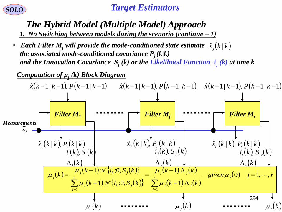
294
SOLO Target Estimators
The Hybrid Model (Multiple Model) Approach
• Each Filter Mj will provide the mode-conditioned state estimate
the associated mode-conditioned covariance Pj (k|k)
and the Innovation Covariance Sj (k) or the Likelihood Function Λj (k) at time k
1. No Switching between models during the scenario (continue – 1)
kkx j |ˆ
Filter M1
1|1,1|1ˆ kkPkkx
kkPkkx |,|ˆ11
k
kSki
1
11 ,
Filter Mj
1|1,1|1ˆ kkPkkx
kkPkkx jj |,|ˆ
k
kSki
j
jj
,
Filter Mr
1|1,1|1ˆ kkPkkx
kkPkkx rr |,|ˆ
k
kSki
r
rr
,
rjgiven
kk
kk
kSik
kSikk jr
j
jj
jj
r
j
jkj
jkj
j ,,10
1
1
,0;1
,0;1
11
N
N
k1 kj kr
Computation of μj (k) Block Diagram
kzMeasurements

295
SOLO Target EstimatorsThe Hybrid Model (Multiple Model) Approach
kz
Filter M1
k
kSki
1
11 ,
Filter Mj
kkPkkx jj |,|ˆ
k
kSki
j
jj
,Filter Mr
k
kSki
r
rr
,
1|1
1|1ˆ
kkP
kkx
MixtureGaussiankkkxkkkxr
j
j
r
j
jj 1|ˆ|ˆ11
rjkkxkkxkkxkkxkkPkkkPT
jj
r
j
jj ,,1|ˆ|ˆ|ˆ|ˆ||1
kkPkkx rr |,|ˆ
1|1
1|1ˆ
kkP
kkx 1|1
1|1ˆ
kkP
kkx
• We have r Gaussian estimates , therefore to obtain the estimate of the system
state and its covariance we can use the results of a Gaussian mixture with r terms
to obtain the Overall State Estimate and its Covariance
1. No Switching between models during the scenario (continue – 2)
kkx j |ˆ
Measurements
rjgiven
kk
kk
kSik
kSikk jr
i
ii
jj
r
i
iki
jkj
j ,,10
1
1
,0;1
,0;1
11
N
N
k1 kj kr kkPkkx |,|ˆ
11
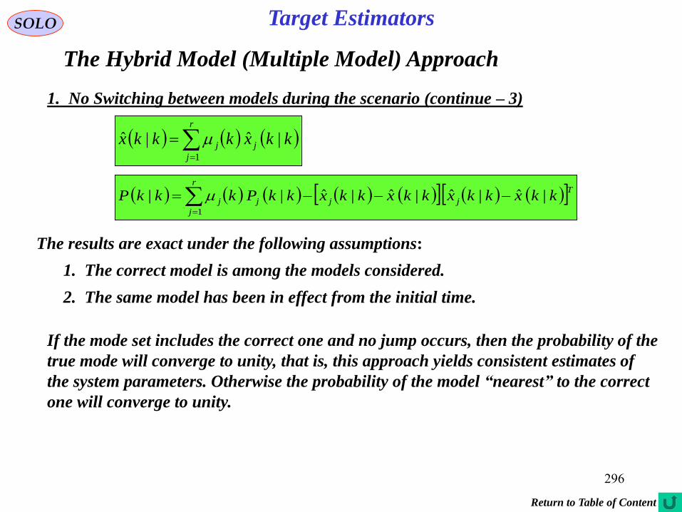
296
SOLO Target Estimators
The Hybrid Model (Multiple Model) Approach
The results are exact under the following assumptions:
1. No Switching between models during the scenario (continue – 3)
r
j
jj kkxkkkx1
|ˆ|ˆ
Tjj
r
j
jj kkxkkxkkxkkxkkPkkkP |ˆ|ˆ|ˆ|ˆ||1
1. The correct model is among the models considered.
2. The same model has been in effect from the initial time.
If the mode set includes the correct one and no jump occurs, then the probability of the
true mode will converge to unity, that is, this approach yields consistent estimates of
the system parameters. Otherwise the probability of the model “nearest” to the correct
one will converge to unity.
Return to Table of Content

297
SOLO Target Estimators
The Hybrid Model (Multiple Model) Approach
2. Switching between models during the scenario
As before the system is modeled by the equations:
kMRvkMkvkMkvkxkMHkz
kMQwkMkwkMkwkxkMFkx
,0;~,,
,0;~,1,11
N
N
where M (k) denotes the model “at time k” – in effect during the sampling period
ending at k. Such systems are called Jump Linear Systems. The mode jump process
is assumed left-continuous (i.e. the impact of the jump starts at tk+)
It is assumed that the mode (model) jump process is a Markov process with known
mode transition probabilities.
Probability of transition from Mi at k-1 to Mj at k is given by the Markov Chain:
ijji MkMMkMPp 1|:
Since, all the possibilities are to jump from i to each of j=1,…,r (including j=i) we
must have
11|11
r
j
ij
r
j
ji MkMMkMPp

298
SOLO Target Estimators
The Hybrid Model (Multiple Model) Approach
2. Switching between models during the scenario (continue – 1)
In this way the number of models running at each new measurement k are:
k = 1, there are r models
k = 2, there are r2 models, since each r models at k = 1 split in new r models
k = 3, there are r3 models, since each r2 models at k = 2 split in new r models
…………………………………………………………………………………….
k, there are rk models.
The number of models grows exponentially making this approach impractical.
The only way to avoid the exponentially increasing number of histories, which have
to be accounted for, is by going to suboptimal techniques.
Return to Table of Content

299
SOLO Target Estimators
The Hybrid Model (Multiple Model) Approach
2. Switching between models during the scenario (continue – 2)
The Interacting Multiple Model (IMM) Algorithm
In the IMM approach, at time k the state estimate is computed under each possible
current model using r filters, with each filter using as start condition (for time k-1)
a different combination of the previous model-conditioned estimates – mixed initial
conditions.
We assume a transition from Mi at k-1 to Mj at k with a predefined probability:
ijji MkMMkMPp 1|: 11|11
r
j
ij
r
j
ji MkMMkMPp
Define
1|1ˆ kkxi - filtered state estimate at scan k-1 for Kalman Filter Model i
1|1 kkPi - covariance matrix at scan k-1 for Kalman Filter Model i
1ki - probability that the target performs as in model state i as
computed just after data is received on scan k-1
1kji - conditional probability that the target made the transition
from state i to state j at scan k-1
r
i
iji
iji
r
i
iij
iij
ji
kp
kp
ZMkMPMkMMkMP
ZMkMPMkMMkMPk
11
1
1
|11|
|11|1

300
SOLO Target Estimators
The Hybrid Model (Multiple Model) Approach
2. Switching between models during the scenario (continue – 3)
The Interacting Multiple Model (IMM) Algorithm (continue – 1)
Tjiji
r
i
ijij
kkxkkxkkxkkx
kkPkkkP
1|1ˆ1|1ˆ1|1ˆ1|1ˆ
1|111|1
00
1
0
For mixed Gaussian distribution we obtain the covariance of mixed initial conditions to be:
Conditional probability that the target made the transition from state i to state j at scan k-1
r
i
iji
iji
r
i
iij
iij
ji
kp
kp
ZMkMPMkMMkMP
ZMkMPMkMMkMPk
11
1
1
|11|
|11|1
rikkxi ,,11|1ˆ Mixing: The IMM algorithm starts with the initial condition
from the filter Mi (k-1), assumed Gaussian distributed, and computes the mixed initial
condition for the filter matched to Mj (k) according to
rjkkxkkkxr
i
ijij ,,11|1ˆ11|1ˆ1
0

301
SOLO Target Estimators
The Hybrid Model (Multiple Model) Approach
2. Switching between models during the scenario (continue – 4)
The Interacting Multiple Model (IMM) Algorithm (continue – 2)
The next step, as described before, is to run the r Kalman Filters and to calculate:
r
j
jkkj
jkkj
j
MZzPk
MZzPkk
1
1:1
1:1
,|1
,|1
rjZMP jj ,,1|0 0
with assumed a prior probabilities
P {zk|Z1:k-1, Mj} is the Likelihood Function Λj (k) of mode j at time k, which, under the
Linear-Gaussian assumptions, is given by
kSkikiPMZzPk jjjjkkj ,0;,|: 1:1 N
j
kjkkj xMHzki ˆwhere Innovation of Filter Mj at time k
jk
T
jk
j
jkj MRMHkkPMHkS |Innovation Covariance of Filter Mj
at time k
r
j
jj kkxkkkx1
|ˆ|ˆ
Tjj
r
j
jj kkxkkxkkxkkxkkPkkkP |ˆ|ˆ|ˆ|ˆ||1
To obtain the estimate of the system state and its covariance we can use the results of a
Gaussian mixture with r terms

302
SOLO Target EstimatorsThe Hybrid Model (Multiple Model) Approach
2. Switching between models during the scenario (continue – 5)
The Interacting Multiple Model (IMM) Algorithm (continue – 3)
IMM Estimation Algorithm Summary
• Interaction: Mixing of the previous cycle mode-conditioned state estimates and
covariance, using the predefined mixing probabilities,
to initialize the current cycle of each mode-conditioned Filter.
1|1,1|1ˆ00 kkPkkx jj
• Mode-Conditioned Filtering: Mixing Calculation of the State Estimate and the
covariance conditioned on a mode being in effect ,
as well as the mode likelihood function , for r parallel Filters.
kkPkkx jj |,|ˆ
kj
• Probability Evaluation: Computation of the mixing and the updated mode
probabilities μj (k) given μj (0), j=1,…,r.
• Overall State Estimate and Covariance: Combination of the latest mode-conditioned
State Estimate and Covariance . kkPkkx |,|ˆ
Tjiji
r
i
ijij
r
i
ijij
kkxkkxkkxkkx
kkPkkkP
rjkkxkkkx
1|1ˆ1|1ˆ1|1ˆ1|1ˆ
1|111|1
,,11|1ˆ11|1ˆ
00
1
0
1
0
rjgivenkkkkk j
r
i
iijjj ,,101/11
r
j
jj kkxkkkx1
|ˆ|ˆ
rjkkxkkxkkxkkxkkPkkkPT
jj
r
j
jj ,,1|ˆ|ˆ|ˆ|ˆ||1

303
SOLO Target EstimatorsThe Hybrid Model (Multiple Model) Approach
kz
2. Switching between models during the scenario (continue – 6)
Filter M1
kkPkkx |,|ˆ11
k
kSki
1
11 ,
Filter Mj
kkPkkx jj |,|ˆ
k
kSki
j
jj
,Filter Mr
k
kSki
r
rr
,
rjgiven
kk
kk
kSik
kSikk jr
i
ii
jj
r
i
iki
jkj
j ,,10
1
1
,0;1
,0;1
11
N
N
k1 kj kr
r
i
iji
iji
ji
kp
kpk
1
1
11
Tjiji
r
i
ijij
r
i
ijij
kkxkkxkkxkkx
kkPkkkP
rjkkxkkkx
1|1ˆ1|1ˆ1|1ˆ1|1ˆ
1|111|1
,,11|1ˆ11|1ˆ
00
1
0
1
0
1|1
1|1ˆ
kkP
kkx
j
j
1ki
1|1
1|1ˆ
0
0
kkP
kkx
j
j
1|1
1|1ˆ
01
01
kkP
kkx
1|1
1|1ˆ
0
0
kkP
kkx
r
r
The Interacting Multiple Model (IMM) Algorithm (continue – 4)
rjip ji ,,1,
r
j
jj kkxkkkx1
|ˆ|ˆ
rjkkxkkxkkxkkxkkPkkkPT
jj
r
j
jj ,,1|ˆ|ˆ|ˆ|ˆ||1
kkPkkx rr |,|ˆ
Measurements

304
SOLO Target EstimatorsThe Hybrid Model (Multiple Model) Approach
2. Switching between models during the scenario (continue – 7)
The Interacting Multiple Model (IMM) Algorithm (continue – 5)
Interaction
(Mixing)
1
1|1ˆ
kkxr
kkx 1|1ˆ
Filter
Mk1
Filter
Mkr
Model
Probability
Update
State
Estimate
Combination
01
1|1ˆ
kkxr
kkx0
1|1ˆ
kz
1
k
r
k
1
|ˆ
kkxr
kkx |ˆ
kkx |ˆk
1k
1|1 kk
IMM Algorithm
jip
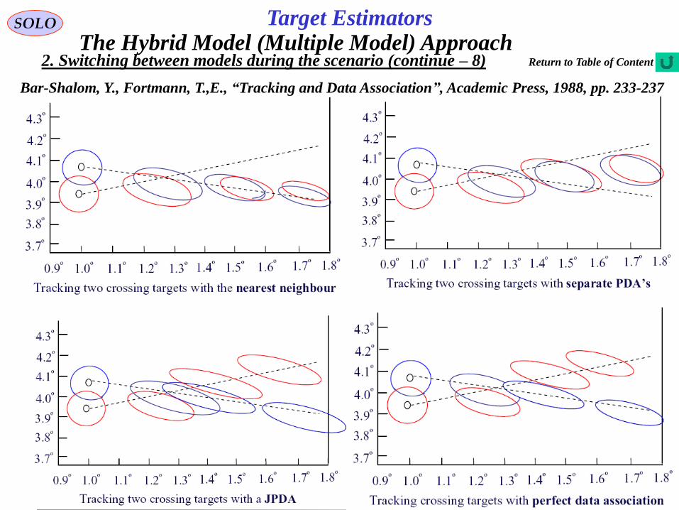
305
SOLO Target EstimatorsThe Hybrid Model (Multiple Model) Approach
2. Switching between models during the scenario (continue – 8)
Bar-Shalom, Y., Fortmann, T.,E., “Tracking and Data Association”, Academic Press, 1988, pp. 233-237
Return to Table of Content

306
SOLO Target EstimatorsThe Hybrid Model (Multiple Model) Approach
2. Switching between models during the scenario (continue – 9)
The IMM-PDAF Algorithm
In cases when we want to detect a Target Maneuver and the Probability of Detection,
PD, is less then 1, and False Alarms are possible we can combine the Interacting
Multiple Model (IMM) Algorithm that allows Target maneuver with the
Probabilistic Data Association Filter (PDAF) that deals with False Alarms, given the
IMM-PDAF Algorithm.
This is done by replacing the Kalman Filters Models of the IMM with PDAF Models.
Interaction
(Mixing)
1
1|1ˆ
kkx r
kkx 1|1ˆ
PDAF
Mk1
PDAF
Mkr
Model
Probability
Update
State
Estimate
Combination
01
1|1ˆ
kkx r
kkx0
1|1ˆ
kz
1
k
r
k
1
|ˆ
kkx r
kkx |ˆ
kkx |ˆk
1k
1|1 kk
IMM-PDAF Algorithm
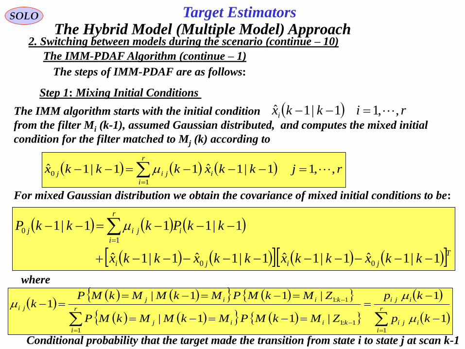
307
SOLO Target EstimatorsThe Hybrid Model (Multiple Model) Approach
2. Switching between models during the scenario (continue – 10)
The IMM-PDAF Algorithm (continue – 1)
The steps of IMM-PDAF are as follows:
Step 1: Mixing Initial Conditions
Tjiji
r
i
ijij
kkxkkxkkxkkx
kkPkkkP
1|1ˆ1|1ˆ1|1ˆ1|1ˆ
1|111|1
00
1
0
For mixed Gaussian distribution we obtain the covariance of mixed initial conditions to be:
rikkxi ,,11|1ˆ The IMM algorithm starts with the initial condition
from the filter Mi (k-1), assumed Gaussian distributed, and computes the mixed initial
condition for the filter matched to Mj (k) according to
rjkkxkkkxr
i
ijij ,,11|1ˆ11|1ˆ1
0
where
Conditional probability that the target made the transition from state i to state j at scan k-1
r
i
iji
iji
r
i
kiij
kiij
ji
kp
kp
ZMkMPMkMMkMP
ZMkMPMkMMkMPk
11
1:1
1:1
1
1
|11|
|11|1

308
SOLO Target EstimatorsThe Hybrid Model (Multiple Model) Approach
2. Switching between models during the scenario (continue – 11)
The IMM-PDAF Algorithm (continue – 2)
The steps of IMM-PDAF are as follows:
Step 2: Mode Conditioning PDAF
riZmiMkZPk kkki ,,1,,|: 1:1
From the r PDAF models we must obtain the likelihood functions Λi(k) i = 1,…,r , for each Model i.
But at PDAF we found that for the Model i:
km
j
kkkjikkkjikkk ZmiMkkZPZmiMkZkPZmiMkZP0
1:11:11:1 ,,,|,,,|,,|
0
,,12
2/exp
,,,|
1
11
1:1
jkV
mjkS
kikSkiPkV
ZmiMkkZP
k
k
m
i
k
i
jii
T
ji
Gi
m
i
kkkji
011
,...,11,,|,
1
1
1:1
jkVPPmPPkVPP
mjkVPPmPPPPZmiMkP
iGiDikGiDiiGiDi
kiGiDikGiDiGiDi
kkkji
2/12/2
12
, kSn
kV i
n
z
n
iz
z
1|ˆ: kkzkzki ijji
and
where kRkHkkPkHkS i
T
iiii 1|:

309
SOLO Target EstimatorsThe Hybrid Model (Multiple Model) Approach
2. Switching between models during the scenario (continue – 12)
The IMM-PDAF Algorithm (continue – 3)
The steps of IMM-PDAF are as follows:
Step 2: Mode Conditioning PDAF (continue – 1)
k
iiii
k
i
iiii
k
k
i
ii
m
j
jii
iGDkGDi
m
i
D
iGDkGD
m
i
m
j
jii
T
ji
i
D
GD
kkki
kebkVPPmPPkSkV
P
kVPPmPPkV
kikSkikS
PPP
ZmiMkZPk
11
1
1
1
1:1
12
1
2/exp2
1
,,|:
From the r PDAF models we obtain the likelihood functions Λi(k) i = 1,…,r , for each Model i.
2/12/2
12
, kSn
kV i
n
z
n
iz
z
1|ˆ: kkzkzki ijji
where
kRkHkkPkHkS i
T
iiii 1|:
kSP
PPb
kikSkie
i
D
GD
i
jii
T
jiji
i
ii 21
:
2/exp:1
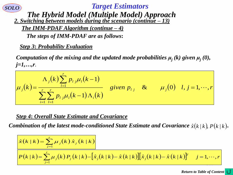
310
SOLO Target EstimatorsThe Hybrid Model (Multiple Model) Approach
2. Switching between models during the scenario (continue – 13)
The IMM-PDAF Algorithm (continue – 4)
The steps of IMM-PDAF are as follows:
Step 3: Probability Evaluation
Computation of the mixing and the updated mode probabilities μj (k) given μj (0),
j=1,…,r.
Combination of the latest mode-conditioned State Estimate and Covariance . kkPkkx |,|ˆ
rjlpgiven
kkp
kpk
k jjlr
i
r
l
iljl
r
l
ljlj
j ,,1,0&
1
1
1 1
1
r
j
jj kkxkkkx1
|ˆ|ˆ
rjkkxkkxkkxkkxkkPkkkPT
jj
r
j
jj ,,1|ˆ|ˆ|ˆ|ˆ||1
Step 4: Overall State Estimate and Covariance
Return to Table of Content

311
Elements of a Basic MTT SystemSOLO
Multi-Target Tracking (MTT) Systems
The task effort of tracking n targets can require substantially more computation resources
than n time the computation resources for tracking a single target, because is difficult to
establish the correspondence between observations and targets (Data Association).
Uncertainties in tracking targets:
• Uncertainties associated with the measurements (target origin).
• Inaccuracies due to the sensor performances (resolution, noise,..)
Tgt. 1
Tgt. 2
Measurement 2
Measurement 1
1. Measurement 1 from target 1 & Measurement 2 from target 2
2. Measurement 1 from target 2 & Measurement 2 from target 1
3. None of the above (False Alarm)
Hypotheses:

312
Elements of a Basic MTT SystemSOLO
Multi-Target Tracking (MTT) Systems
Association Hypothesis 1
Measurement 2
Measurement 1
t1 t2 t3
Measurement
2
Measurement
1
t1 t2 t3
Measureme
nt 2
Measureme
nt 1
t
1
t
2
t
3
Measureme
nt 2
Measureme
nt 1
t
1
t
2
t
3
Association Hypothesis 2 Association Hypothesis 3

313
Elements of a Basic MTT SystemSOLO
Alignment: Referencing of sensor data to a common time and spatial origin.
Association: Using a metric to compare tracks and data reports from different
sensors to determine candidates for the fusion process.
Correlation: Processing of the tracks and reports resulting from association
to determine if they belong to a common object and thus aid in
detecting, classifying and tracking the objects of interest.
Estimation: Predicting an object’s future position by updating the state vector
and error covariance matrix using the results of the correlation
process.
Classification: Assessing the tracks and object discrimination data to determine
target type, lethality, and threat priority.
Cueing: Feedback of threshold, integration time, and other data processing
parameters or information about areas over which to conduct a more
detailed search, based on the results of the fusion process.
Return to Table of Content
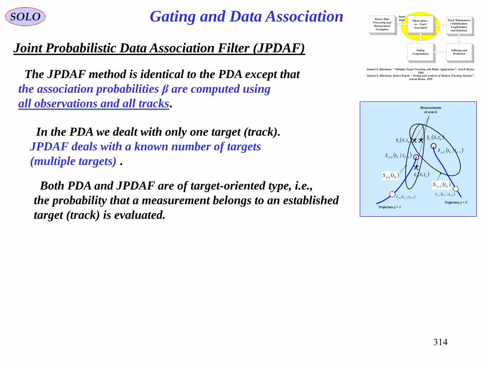
314
Sensor Data
Processing and
Measurement
Formation
Observation -
to - Track
Association
Input
Data Track Maintenance
( Initialization,
Confirmation
and Deletion)
Filtering and
Prediction
Gating
Computations
Samuel S. Blackman, " Multiple-Target Tracking with Radar Applications", Artech House,
1986Samuel S. Blackman, Robert Popoli, " Design and Analysis of Modern Tracking Systems",
Artech House, 1999
ktxz ,1
kj tS 2
11 |ˆ kkj ttz
ktxz ,2 ktxz ,3
12 |ˆ kkj ttz
kj tS 1
Trajectory j = 2
Trajectory j = 1
Measurements
at scan k
212 |ˆ kkj ttz
211 |ˆ kkj ttz
SOLO
Joint Probabilistic Data Association Filter (JPDAF)
The JPDAF method is identical to the PDA except that
the association probabilities β are computed using
all observations and all tracks.
Gating and Data Association
In the PDA we dealt with only one target (track).
JPDAF deals with a known number of targets
(multiple targets) .
Both PDA and JPDAF are of target-oriented type, i.e.,
the probability that a measurement belongs to an established
target (track) is evaluated.
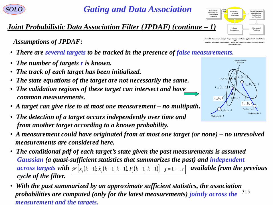
315
Sensor Data
Processing and
Measurement
Formation
Observation -
to - Track
Association
Input
Data Track Maintenance
( Initialization,
Confirmation
and Deletion)
Filtering and
Prediction
Gating
Computations
Samuel S. Blackman, " Multiple-Target Tracking with Radar Applications", Artech House,
1986Samuel S. Blackman, Robert Popoli, " Design and Analysis of Modern Tracking Systems",
Artech House, 1999
ktxz ,1
kj tS 2
11 |ˆ kkj ttz
ktxz ,2 ktxz ,3
12 |ˆ kkj ttz
kj tS 1
Trajectory j = 2
Trajectory j = 1
Measurements
at scan k
212 |ˆ kkj ttz
211 |ˆ kkj ttz
SOLO
Joint Probabilistic Data Association Filter (JPDAF) (continue – 1)
Assumptions of JPDAF:
Gating and Data Association
• There are several targets to be tracked in the presence of false measurements.
• The number of targets r is known.
• The track of each target has been initialized.
• The state equations of the target are not necessarily the same.
• The validation regions of these target can intersect and have
common measurements.
• A target can give rise to at most one measurement – no multipath.
• The detection of a target occurs independently over time and
from another target according to a known probability.
• A measurement could have originated from at most one target (or none) – no unresolved
measurements are considered here.
rjkkPkkxkx jjj ,,11|1,1|1ˆ;1 N
• The conditional pdf of each target’s state given the past measurements is assumed
Gaussian (a quasi-sufficient statistics that summarizes the past) and independent
across targets with available from the previous
cycle of the filter.
• With the past summarized by an approximate sufficient statistics, the association
probabilities are computed (only for the latest measurements) jointly across the
measurement and the targets.

316
Sensor Data
Processing and
Measurement
Formation
Observation -
to - Track
Association
Input
Data Track Maintenance
( Initialization,
Confirmation
and Deletion)
Filtering and
Prediction
Gating
Computations
Samuel S. Blackman, " Multiple-Target Tracking with Radar Applications", Artech House,
1986Samuel S. Blackman, Robert Popoli, " Design and Analysis of Modern Tracking Systems",
Artech House, 1999
ktxz ,1
kj tS 2
11 |ˆ kkj ttz
ktxz ,2 ktxz ,3
12 |ˆ kkj ttz
kj tS 1
Trajectory j = 2
Trajectory j = 1
Measurements
at scan k
212 |ˆ kkj ttz
211 |ˆ kkj ttz
SOLO
Joint Probabilistic Data Association Filter (JPDAF) (continue -2)
• At the current time k we define the set of validated measurements:
Gating and Data Association
km
ii kzkZ1
Example: From Figure we can see 3 measurements (mk=3)
,,, 321 kzkzkzkZ
• We also have r predefined target (tracks) i=1,…,r
Example: From Figure we can see 2 tracks (r = 2)
• From the validated measurements and their position relative
to track gates we define the Validation Matrix Ω that consists of
binary elements (0 or 1) indicating if measurement j has been validated for track j
(is inside the j Gate). Index i = 0 (no track) indicates a false alarm (clutter) origin,
which is possible for each measurement.
Example: From Figure
3
2
1
101
111
011
ˆ
210
meas
meas
meas
ji
ij
Measurement 1 can be FA or due track1, not track2
Measurement 2 can be FA or due track1, or track2
Measurement 3 can be FA or due track2, not track1
tracks

317
Sensor Data
Processing and
Measurement
Formation
Observation -
to - Track
Association
Input
Data Track Maintenance
( Initialization,
Confirmation
and Deletion)
Filtering and
Prediction
Gating
Computations
Samuel S. Blackman, " Multiple-Target Tracking with Radar Applications", Artech House,
1986Samuel S. Blackman, Robert Popoli, " Design and Analysis of Modern Tracking Systems",
Artech House, 1999
ktxz ,1
kj tS 2
11 |ˆ kkj ttz
ktxz ,2 ktxz ,3
12 |ˆ kkj ttz
kj tS 1
Trajectory j = 2
Trajectory j = 1
Measurements
at scan k
212 |ˆ kkj ttz
211 |ˆ kkj ttz
SOLO
Joint Probabilistic Data Association Filter (JPDAF) (continue -3)
Gating and Data Association
• Define the Joint Association Events θ (Hypotheses) using the
Validation Matrix
Example: From Figure
3
2
1
111
111
011
ˆ
210
meas
meas
meas
ji
ij
tracks
Validation Matrix
ijˆˆ
Hypotesis
Number
Track Number
1 2
Comments
1 0 0 All measurements are False Alarms
2 1 0 Measurement # 1 due to target # 1, other are F.A.
3 2 0 Measurement # 2 due to target # 1, other are F.A.
4 3 0 Measurement # 3 due to target # 1, other are F.A.
5 0 2 Measurement # 2 due to target # 2, other are F.A.
6 1 2 Measurement # 1 due to target # 1, #2 due target #2.
7 3 2 Measurement # 3 due to target # 1, #2 due target #2.
8 0 3 Measurement # 3 due to target # 2, other are F.A
9 1 3 Measurement # 2 due to target # 1, #3due target #2.
10 2 3 Measurement # 1 due to target # 1, #3 due target #2.
Those are all the Hypotheses
(exhaustive) defined by the
Validation Matrix (or Figure)
Run This

318
Sensor Data
Processing and
Measurement
Formation
Observation -
to - Track
Association
Input
Data Track Maintenance
( Initialization,
Confirmation
and Deletion)
Filtering and
Prediction
Gating
Computations
Samuel S. Blackman, " Multiple-Target Tracking with Radar Applications", Artech House,
1986Samuel S. Blackman, Robert Popoli, " Design and Analysis of Modern Tracking Systems",
Artech House, 1999
ktxz ,1
kj tS 2
11 |ˆ kkj ttz
ktxz ,2 ktxz ,3
12 |ˆ kkj ttz
kj tS 1
Trajectory j = 2
Trajectory j = 1
Measurements
at scan k
212 |ˆ kkj ttz
211 |ˆ kkj ttz
SOLO
Joint Probabilistic Data Association Filter (JPDAF) (continue -4)
Gating and Data Association
• Define the Joint Association Events θ (Hypotheses) using the
Validation Matrix
Example: From Figure
3
2
1
111
111
011
ˆ
210
meas
meas
meas
ji
ij
tracks
Validation Matrix
ijˆˆ
Those are all the Hypotheses
(exhaustive) defined by the
Validation Matrix (or Figure)
O\H 1 2 3 4 5 6 7 8 9 10
O1 0 T1 0 0 0 T1 0 0 T1 0
O2 0 0 T1 0 T2 T2 T2 0 0 T1
O3 0 0 0 T1 0 0 T1 T2 T2 T2
hypothesis number
obs
Run This

319
Sensor Data
Processing and
Measurement
Formation
Observation -
to - Track
Association
Input
Data Track Maintenance
( Initialization,
Confirmation
and Deletion)
Filtering and
Prediction
Gating
Computations
Samuel S. Blackman, " Multiple-Target Tracking with Radar Applications", Artech House,
1986Samuel S. Blackman, Robert Popoli, " Design and Analysis of Modern Tracking Systems",
Artech House, 1999
SOLO
We have n stored tracks that have predicted measurements
and innovations co variances at scan k given by:
At scan k+1 we have m sensor reports (no more than one report
per target)
njkSkkz jj ,,1,1|ˆ
set of all sensor reports on scan k mk zzZ ,,1
H – a particular hypothesis (from a complete set S of hypotheses)
connecting r (H) tracks to r measurements.
We want to compute:
HPHZPcHPHZP
HPHZPZHP k
SH
k
kk |
1
|
||
Joint Probabilistic Data Association Filter (JPDAF) (continue -5)
Gating and Data Association

320
Sensor Data
Processing and
Measurement
Formation
Observation -
to - Track
Association
Input
Data Track Maintenance
( Initialization,
Confirmation
and Deletion)
Filtering and
Prediction
Gating
Computations
Samuel S. Blackman, " Multiple-Target Tracking with Radar Applications", Artech House,
1986Samuel S. Blackman, Robert Popoli, " Design and Analysis of Modern Tracking Systems",
Artech House, 1999
SOLO
We have several tracks defined by the predicted measurements
and innovations co variances
!m
Vem
m
V
FA
The probability density function of the false alarms, in the search volume V, in terms of
their spatial density λ , is given by aPoisson Distribution:
njkSkkz jj ,,11,|1ˆ
Not all the measurements are from a real target but are from
False Alarms. The common mathematical model for such false
measurements is that they are:
• uniformly spatially distributed
• independent across time
• this is the residual clutter (the constant clutter, if any, is not considered.
m is the number of measurements in scan k+1
V
orAlarmFalsezP i
1TargetNew|
Because of the uniformly space distribution in the search Volume, we have:
False Alarm Models
Gating and Data Association
Joint Probabilistic Data Association Filter (JPDAF) (continue - 6)
We can use different probability densities for false alarms (λFA) and for new targets (λNT)

321
Sensor Data
Processing and
Measurement
Formation
Observation -
to - Track
Association
Input
Data Track Maintenance
( Initialization,
Confirmation
and Deletion)
Filtering and
Prediction
Gating
Computations
Samuel S. Blackman, " Multiple-Target Tracking with Radar Applications", Artech House,
1986Samuel S. Blackman, Robert Popoli, " Design and Analysis of Modern Tracking Systems",
Artech House, 1999
SOLO
H – a particular hypothesis (from a complete set S of hypotheses)
connecting r (H) tracks to r measurements and assuming m-r false alarms or new targets.
r
V
rm
li
iji
T
ijm
l
lk
rkm
kk
VS
zzSzzHzpHZP
1
/1
1
1
1
1
2
2/ˆˆexp||
HPHZPcHPHZP
HPHZPZHP k
SH
k
kk |
1
|
||
mk zzZ ,,11 P (Zk|H) - probability of the measurements
given that hypothesis H is true.
km
j
j
tindependen
tsmeasuremenmk HzPHzzPHZP
1
1 ||,,|
where:
itracktoconnectedjtmeasuremenS
zSzSz
orAlarmFalseistmeasuremenjifV
HzP
i
ii
T
i
ii
j
2
2/ˆzˆzexp,ˆ;z
TargetNew1
|j
1
j
jN
Gating and Data Association
Joint Probabilistic Data Association Filter (JPDAF) (continue - 7)

322
Sensor Data
Processing and
Measurement
Formation
Observation -
to - Track
Association
Input
Data Track Maintenance
( Initialization,
Confirmation
and Deletion)
Filtering and
Prediction
Gating
Computations
Samuel S. Blackman, " Multiple-Target Tracking with Radar Applications", Artech House,
1986Samuel S. Blackman, Robert Popoli, " Design and Analysis of Modern Tracking Systems",
Artech House, 1999
SOLO
HPHZPcHPHZP
HPHZPZHP k
SH
k
kk |
1
|
||
P (H) – probability of hypothesis H connecting tracks i1,…,ir
to measurements j1,…,jr from mk sensor reports:
kkFA
tracks
r
tracks
r
tsmeasuremen
r mPrmPiiPiijjPHP
,,,,|,, 111
!
!
11
1,,|,, 11
m
rm
rmmmiijjP
tracks
r
tsmeasuremen
r
probability of connecting tracks i1,…,ir
to measurements j1,…,jr
DetectingNot
m
iiii
D
iiDetecting
r
D
tracks
r
k
r
i
r
jPPiiP
,,1
,,
1
1
1
1
1,,
probability of detecting only i1,…,ir
targets
V
k
rm
kFAkFA erm
VrmrmP
k
!
for (m-r) False Alarms or New Targets assume Poisson
Distribution with density λ over search volume V of
(mk-r) reports
kmP probability of exactly mk reports
where:
Gating and Data Association
Joint Probabilistic Data Association Filter (JPDAF) (continue - 8)

323
Sensor Data
Processing and
Measurement
Formation
Observation -
to - Track
Association
Input
Data Track Maintenance
( Initialization,
Confirmation
and Deletion)
Filtering and
Prediction
Gating
Computations
Samuel S. Blackman, " Multiple-Target Tracking with Radar Applications", Artech House,
1986Samuel S. Blackman, Robert Popoli, " Design and Analysis of Modern Tracking Systems",
Artech House, 1999
SOLO
where:
HPHZPc
ZHP kk |1
|
r
i
iji
T
ij
rmm
l
lk
S
zzSzz
VHzpHZP
kk
1
1
1 2
2/ˆˆexp1||
k
V
k
rm
DetectingNot
m
iiii
D
iiDetecting
r
D
k
k mPerm
VPP
m
rmHP
kk
r
i
r
j
!
1!
!
,,1
,,
1
1
1
Gating and Data Association
Joint Probabilistic Data Association Filter (JPDAF) (continue - 9)
k
V
k
rm
DetectingNot
m
iiii
D
iiDetecting
r
D
k
kr
i
iji
T
ij
rm
m
l
lkk
mPerm
VPP
m
rm
S
zzSzz
Vc
HzpHPHZPc
ZHP
kk
r
i
r
j
k
k
!1
!
!
2
2/ˆˆexp11
||1
|
,,1
,,
11
1
1
1
1
DetectingNot
m
iiii
D
iiDetecting
r
D
rmr
i
iji
T
ij
c
k
k
V k
r
i
r
j
k PPS
zzSzzmP
m
e
c
,,1
,,
11
1
/11
1
1
12
2/ˆˆexp
!
1

324
Sensor Data
Processing and
Measurement
Formation
Observation -
to - Track
Association
Input
Data Track Maintenance
( Initialization,
Confirmation
and Deletion)
Filtering and
Prediction
Gating
Computations
Samuel S. Blackman, " Multiple-Target Tracking with Radar Applications", Artech House,
1986Samuel S. Blackman, Robert Popoli, " Design and Analysis of Modern Tracking Systems",
Artech House, 1999
ktxz ,1
kj tS 2
11 |ˆ kkj ttz
ktxz ,2 ktxz ,3
12 |ˆ kkj ttz
kj tS 1
Trajectory j = 2
Trajectory j = 1
Measurements
at scan k
212 |ˆ kkj ttz
211 |ˆ kkj ttz
SOLO
The probabilities of each hypothesis is given by:
DetectingNot
m
iiii
D
iiDetecting
r
D
rmr
g
i
iji
T
ij
k
k
r
i
r
j
k
ji
PPS
zzSzz
cZHP
,,1
,,
11
1
1
1
12
2/ˆˆexp
'
1|
Gating and Data Association
Joint Probabilistic Data Association Filter (JPDAF) (continue -10)
Hypotes
is
Number
Track
Number
1 2
Number
of
confirmed
Tracks r
Number
of
FA mk-r
Hypothesis Probability
1 0 0 0 3
2 1 0 1 2
3 2 0 1 2
4 3 0 1 2
5 0 2 1 2
6 1 2 2 1
7 3 2 2 1
8 0 3 1 2
9 1 3 2 1
10 2 3 2 1
Example: Number of observations mk=3 with equal PD
'/1|33
1 cPZHP Dk
'/1|22
112 cPPgZHP DDk
'/1|22
123 cPPgZHP DDk
'/1|22
134 cPPgZHP DDk
'/1|22
225 cPPgZHP DDk
'/1|2
22116 cPPggZHP DDk
'/1|2
22137 cPPggZHP DDk
'/1|22
238 cPPgZHP DDk
'/1|2
23119 cPPggZHP DDk
'/1|2
231210 cPPggZHP DDk
c’ is defined by
requiring:
P (H1|Zk)+…
…+P (H10|Zk)
=1
i
iji
T
ij
ji
S
zzSzzg
2
2/ˆˆexp:
1
Define:i – track index
j – measurement index
Run This
(First Display)
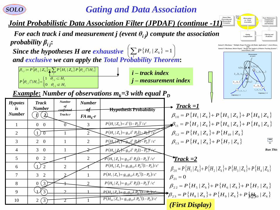
325
Sensor Data
Processing and
Measurement
Formation
Observation -
to - Track
Association
Input
Data Track Maintenance
( Initialization,
Confirmation
and Deletion)
Filtering and
Prediction
Gating
Computations
Samuel S. Blackman, " Multiple-Target Tracking with Radar Applications", Artech House,
1986Samuel S. Blackman, Robert Popoli, " Design and Analysis of Modern Tracking Systems",
Artech House, 1999
ktxz ,1
kj tS 2
11 |ˆ kkj ttz
ktxz ,2 ktxz ,3
12 |ˆ kkj ttz
kj tS 1
Trajectory j = 2
Trajectory j = 1
Measurements
at scan k
212 |ˆ kkj ttz
211 |ˆ kkj ttz
SOLO
For each track i and measurement j (event θi j) compute the association
probability βi j:
Gating and Data Association
Joint Probabilistic Data Association Filter (JPDAF) (continue -11)
Hypotes
is
Number
Track
Number
1 2
Number
of
confirmed
Tracks r
Number
of
FA mk-r
Hypothesis Probability
1 0 0 0 3
2 1 0 1 2
3 2 0 1 2
4 3 0 1 2
5 0 2 1 2
6 1 2 2 1
7 3 2 2 1
8 0 3 1 2
9 1 3 2 1
10 2 3 2 1
Example: Number of observations mk=3 with equal PD
'/1|33
1 cPZHP Dk
'/1|22
112 cPPgZHP DDk
'/1|22
123 cPPgZHP DDk
'/1|22
134 cPPgZHP DDk
'/1|22
225 cPPgZHP DDk
'/1|2
22116 cPPggZHP DDk
'/1|2
22137 cPPggZHP DDk
'/1|22
238 cPPgZHP DDk
'/1|2
23119 cPPggZHP DDk
'/1|2
231210 cPPggZHP DDk
Since the hypotheses H are exhaustive
and exclusive we can apply the Total Probability Theorem:
lji
lji
lji
l
ljiklkjiji
H
HHP
HPZHPZP
0
1
||:
i – track index
j – measurement index
Track =1
kkk ZHPZHPZHP ||| 85101
kkk ZHPZHPZHP ||| 96211
kk ZHPZHP || 10321
kk ZHPZHP || 7431
Track =2
kkkk ZHPZHPZHPZHP |||| 432102
021
kkk ZHPZHPZHP ||| 76522
kkk ZHPZHPZHP ||| 109832
1|
l
kl ZHP
Run This
(First Display)

326
Sensor Data
Processing and
Measurement
Formation
Observation -
to - Track
Association
Input
Data Track Maintenance
( Initialization,
Confirmation
and Deletion)
Filtering and
Prediction
Gating
Computations
Samuel S. Blackman, " Multiple-Target Tracking with Radar Applications", Artech House,
1986Samuel S. Blackman, Robert Popoli, " Design and Analysis of Modern Tracking Systems",
Artech House, 1999
ktxz ,1
kj tS 2
11 |ˆ kkj ttz
ktxz ,2 ktxz ,3
12 |ˆ kkj ttz
kj tS 1
Trajectory j = 2
Trajectory j = 1
Measurements
at scan k
212 |ˆ kkj ttz
211 |ˆ kkj ttz
SOLO
• Computation of Hypotheses Probabilities:
Gating and Data Association
Joint Probabilistic Data Association Filter (JPDAF) (continue -12)
Summary:
zGji
jii
T
jiji
ijji
kj
nPd
kikSkid
kkzkzki
riFor
mjkz
,
1|ˆ
,,1
,,2,1
2
12
• Calculation of Innovation and Measurement Validation for each Measurement versus
each Track
• Definition of all Hypotheses (exhausive & exclusive)
O\H 1 2 3 4 5 6 7 8 9 10
O1 0 T1 0 0 0 T1 0 0 T1 0
O2 0 0 T1 0 T2 T2 T2 0 0 T1
O3 0 0 0 T1 0 0 T1 T2 T2 T2
hypothesis number l
obs
DetectingNot
m
iiii
D
iiDetecting
r
D
rmr
g
i
iji
T
ij
k
k
r
i
r
j
k
ji
PPS
zzSzz
cZHP
,,1
,,
11
1
1
1
12
2/ˆˆexp
'
1|
1|
l
kl ZHP
Run This
(Second Display)

327
Sensor Data
Processing and
Measurement
Formation
Observation -
to - Track
Association
Input
Data Track Maintenance
( Initialization,
Confirmation
and Deletion)
Filtering and
Prediction
Gating
Computations
Samuel S. Blackman, " Multiple-Target Tracking with Radar Applications", Artech House,
1986Samuel S. Blackman, Robert Popoli, " Design and Analysis of Modern Tracking Systems",
Artech House, 1999
SOLO Gating and Data Association
Joint Probabilistic Data Association Filter (JPDAF) (continue -13)
Summary (continue – 1):
• Compute Combined Innovation for each Trackriii
m
itrackjj
jijii ,,1
`1
• Covariance Prediction for each Track
rikQkFkkPkFkkP i
T
iiii ,,1111|11|
• Innovation Covariance for each Track
rikRkHkkPkHkS i
T
iiii ,,11|
• For each track i and measurement j (event θi j) compute the association
probability βi j:
l
ljiklkjiji HPZHPZP ||:i – track index
j – measurement index
lji
lji
ljiH
HHP
0
1
• Filter Gain for each Track rikSkHkkPkK i
T
iii ,,11|1
• Update State Estimation for each Track rikikKkkxkkx iiii ,,11|ˆ|ˆ
• Update State Covariance for each Track
kKiiiikKkdP
rikdPkkPkHkKIkkPkkP
T
i
T
ii
m
itrackjj
T
jijijiii
iiiiiiii
k
1
00 ,,11|11||

328
SOLO
1|1 kkPi
State Covariance
kRkHkkPkHkS i
T
iiii 1|
Innovation Covariance
111|111| kQkFkkPkFkkP i
T
iiii
Covariance of Predicted State
kSkHkkPkK i
T
iii
11|
Filter Gain
kKkikikikikKkPdT
i
T
ii
m
itrackjj
T
jijijiii
k
&
1
Effect of Measurement Origin
on State Covarriance
Update State Covariance
kPdkkPkHkKI
kkPkkP
iiiii
iii
1|1
1||
0
0
Update State Estimation
kikKkkxkkx iiii 1||
kSi
ki ji
ji
kii
kz i
One Cycle of
JPDAF for Track i
Measurements
Evaluation of Association Probabilities
Predicted Measurements
1|1|ˆ kkxkHkkz iii
Calculation of Innovation and
Measurement Validation
State Estimation for Track i
1|1 kkxi
Predicted State of Track i
1|111| kkxkFkkx iii
zGji
jii
T
jiji
ijji
kj
nPd
kikSkid
kkzkzki
riFor
mjkz
,
1|ˆ
,,1
,,2,1
2
12
Definition of all Hypotheses H
and their Probabilities
l
ljiklkjiji HPZHPZP ||:
DetectingNot
m
iiii
D
iiDetecting
r
D
rmr
g
i
iji
T
ij
k
k
r
i
r
j
k
ji
PPS
zzSzz
cZHP
,,1
,,
11
1
1
1
12
2/ˆˆexp
'
1|
Combined Innovation
km
itrackjj
jijii kiki1
Gating and Data Association
Joint Probabilistic Data Association Filter (JPDAF) (continue -14)
Return to Table of Content

329
SOLO Multi Hypothesis Tracking (MHT)
Assumptions of MHT
ktxz ,1
kj tS 2
11 |ˆ kkj ttz
ktxz ,2 ktxz ,3
12 |ˆ kkj ttz
kj tS 1
Trajectory j = 2
Trajectory j = 1
Measurements
at scan k
212 |ˆ kkj ttz
211 |ˆ kkj ttz
• There is several targets to be tracked in the presence of false measurements.
• The number of targets r is unknown.
• The track of each target has to bee initialized.
• The state equations of the targets are the same.
• The validation regions of these targets can intersect and have
common measurements.
• A target can give rise to at most one measurement – no multipath.
• The detection of a target occurs independently over time and
from another target according to a known probability.
• A measurement could have originated from at most one target (or none) – no unresolved
measurements are considered here.
rjkkPkkxkx jjj ,,11|1,1|1ˆ;1 N
• The conditional pdf of each target’s state given the past measurements is assumed
Gaussian (a quasi-sufficient statistics that summarizes the past) and independent
across targets with available from the previous
cycle of the filter.
• The origin of each sequence of measurements is considered.
• At each sampling time any measurement can originated from:
- an established track
- a new target (with a Poisson Probability λNT)
- a false alarm (with a Poisson Probability λFA)

330
SOLO Multi Hypothesis Tracking (MHT)
MHT Algorithm Steps
• The Hypotheses of the current time are obtained from:
• The Set of Hypotheses at the previous time augmented with
• All the Feasible Associations of the Present Measurements (Extensive and Exhaustive).
• The Probability of each Hypothesis is evaluated assuming:.
• measurements associated with a track are Gaussian distributed
around the predicted location of the corresponding track’s
measurement.
• false measurements are uniformly distributed in the surveillance
region and appear according to a fixed rate (λFA) Poisson process.
• The State Estimation for each Hypothesized Track is obtained from a Standard Filter.
• The selection of the Most Probable Hypothesis amounts to an Exhaustive Search
over the Set of All Feasible Hypotheses.
ktxz ,1
11 |ˆ kkj ttz
ktxz ,2 ktxz ,3
kj tS 1
Trajectory j = 1
Measurements
at scan k
211 |ˆ kkj ttz
• new targets are uniformly distributed in the surveillance
region (or according to some other PDF) and appear according to
a fixed rate (λNT) Poisson process.
• An elaborate Hypothesis Management is needed.

331
SOLO Multi Hypothesis Tracking (MHT)
k=0
measurements
1 2
1 1
k=1
Plots
1,2
1 1 3
1 1 4
1 2 4
1 2 3
k=2
Plots
3,4
k=3
Plots
5,6 1 1 3 5
1 1 3 6
1 1 4 5
1 1 4 6
1 2 3 5
1 2 3 6
1 2 4 5
1 2 4 6
Hypoth
eses
MHT tree
At scan k we have m sensor reports (no more than one report
per target)
set of all sensor reports on scan k+1 mk zzZ ,,1
Hl – a particular hypothesis (from a complete set S of
hypotheses) connecting r (H) tracks to r measurements. Measureme
nt 2
Measureme
nt 1
t1 t2 t3
Association
Hypothesis 1
Measureme
nt 2
Measureme
nt 1
t
1
t
2
t
3 Association Hypothesis 2
Measureme
nt 2
Measureme
nt 1
t
1
t
2
t
3Association Hypothesis 3
Measureme
nt 2
Measureme
nt 1
t1 t2 t3

332
SOLO Multi Hypothesis Tracking (MHT)
Donald B. Reid
PhD A&A Stanford U.
1972
Receive New Data Set
Perform Target Time
Update
Form new clusters,
identifying which targets
and measurements are
associated with each
cluster.
Initialization
(A priori targets)
Clusters
Hypotheses
Generation
Form new set of hypotheses,
calculate their probabilities, and
perform a target measurement
for each hypothesis of each
cluster.
Simplify hypothesis matrix of each
cluster. Transfer tentative targets
With unity probability to confirmed
Target category. Create new clusters
For confirmed targets no longer in
Hypothesis matrix.
Mash
Stop
Reduce number of
hypotheses by
elimination or
combination,.
Reduce
Return to Next
Data Set
Flow Diagram of
Multi Target Tracking
Algorithms
(Reid 1979)

333
SOLO Multi Hypothesis Tracking (MHT)
MHT Implementation Issues
• Need to manage Hypotheses to keep their number reasonable small.
• Limit the History (the deep of hypotheses is N last scans)
• Combining and pruning of Hypotheses:
- Retain only hypotheses with probability above certain threshold.
- Combine hypotheses with last M association in common.
• Clustering:
- Cluster is a set of tracks with common measurements and association
hypotheses; hypotheses sets from different clusters are evaluated separately.
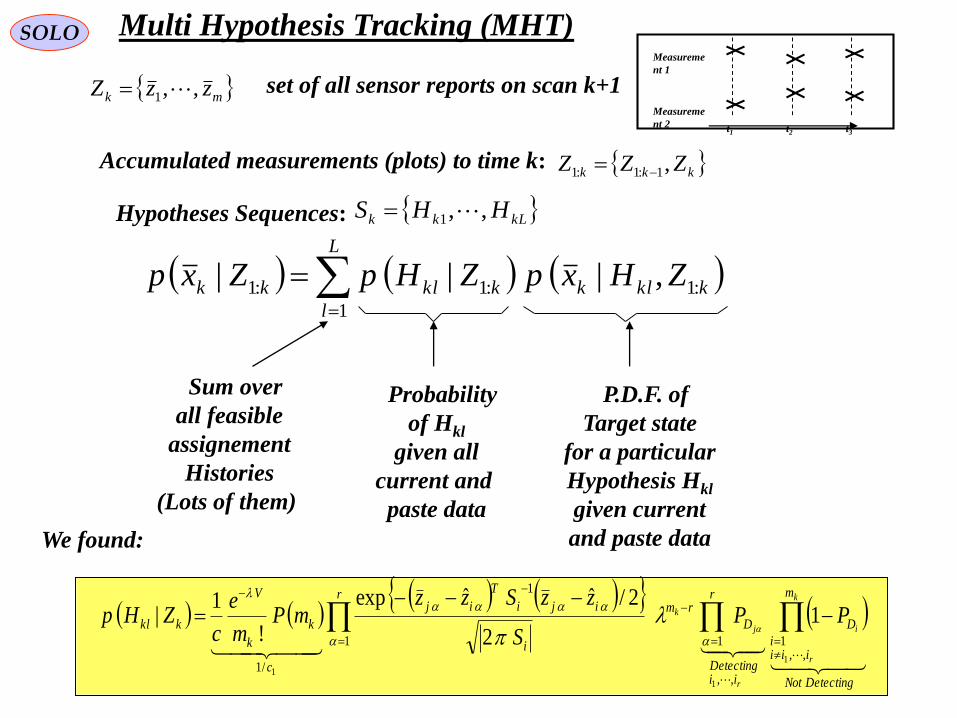
334
SOLO Multi Hypothesis Tracking (MHT)
set of all sensor reports on scan k+1 mk zzZ ,,1
Sum over
all feasible
assignement
Histories
(Lots of them)
Measureme
nt 2
Measureme
nt 1
t1 t2 t3
Accumulated measurements (plots) to time k: kkk ZZZ ,1:1:1
Hypotheses Sequences: kLkk HHS ,,1
L
l
kklkkklkk ZHxpZHpZxp1
:1:1:1 ,|||
Probability
of Hkl
given all
current and
paste data
P.D.F. of
Target state
for a particular
Hypothesis Hkl
given current
and paste data
DetectingNot
m
iiii
D
iiDetecting
r
D
rmr
i
iji
T
ij
c
k
k
V
kkl
k
r
i
r
j
k PPS
zzSzzmP
m
e
cZHp
,,1
,,
11
1
/11
1
1
12
2/ˆˆexp
!
1|
We found:

335
Sensor # 1
Sensor # 2
Estimator
1v
xx
1z
2z2v
SOLO
Multi-Sensor Estimate
Consider a system comprised of two sensors,
each making a single measurement, zi (i=1,2),
of a constant, but unknown quantity, x, in the
presence of random, dependent, unbiased
measurement errors, vi (i=1,2). We want to design an optimal estimator that
combines the two measurements.
110
01122112
2
2
22222
2
1
2
11111
vEvvEvE
vEvEvEvxz
vEvEvEvxz
In absence of any other information, we chose an estimator that combines, linearly,
the two measurements:
2211ˆ zkzkx
where k1 and k2 must be found such that:
1. The Estimator is Unbiased: 0~ˆ xExxE
011
~ˆ
2121
0
22
0
11
2211
xkkxEkkvEkvEk
xvxkvxkExExxE
x
121 kk
Sensors Fusion

336
Sensor # 1
Sensor # 2
Estimator
1v
xx
1z
2z2v
SOLO
Multi-sensor Estimate (continue – 1)
2211ˆ zkzkx
where k1 and k2 must be found such that:
1. The Estimator is Unbiased: 0~ˆ xExxE 121 kk
2. Minimize the Mean Square Estimation Error: 2
,
2
,
~minˆmin2121
xExxEkkkk
2111
2
2
2
1
2
1
2
12111
2
2
2
1
2
1
2
1
2
2111
2
2111
2
,
121min121min
1min1minˆmin
1
212
22
1
1
1121
kkkkvvEkkvEkvEk
vkvkExvxkvxkExxE
kk
kkkk
0212122121 211
2
21
2
112111
2
2
2
1
2
1
2
1
1
kkkkkkk
k
21
2
2
2
1
21
2
112
21
2
2
2
1
21
2
21
2
ˆ1ˆ&2
ˆ
kkk
2
2
2
1
21
2
2
2
1
22
2
2
12 ,2
1~min
xE Reduction of Covarriance Error
Estimator:
Sensors Fusion

337
Sensor # 1
Sensor # 2
Estimator
1v
xx
1z
2z2v
SOLO
Multi-sensor Estimate (continue – 2)
21
2
1
1
2
2
2
1
1
2
1
1
2
211
2
1
1
2
2
2
1
1
2
1
1
2
1
2
21
2
2
2
1
21
2
11
21
2
2
2
1
21
2
2
22
22ˆ
zz
zzx
2
2
2
11
2
1
1
2
2
2
1
2
21
2
2
2
1
22
2
2
12 ,2
1
2
1~min
xE
1. Uncorrelated Measurement Noises (ρ =0)
2
12
2
2
1
2
21
12
2
2
1
2
1ˆ zzx
0~min 2 xE
2. Fully Correlated Measurement Noises (ρ =±1)
3. Perfect Sensor (σ 1 = 0)
1ˆ zx 0~min 2 xE The estimator will use the perfect sensor as expected.
21
2
1
1
1
211
2
1
1
1
1ˆ zzx
Sensors Fusion

338
Sensor # 1
Sensor # 2 Estimator
1v
xx
1z
2z2v
Sensor # n
nznv
SOLO
Multi-sensor Estimate (continue – 3)
Consider a system comprised of n sensors,
each making a single measurement, zi (i=1,2,…,n),
of a constant, but unknown quantity, x, in the
presence of random, dependent, unbiased
measurement errors, vi (i=1,2,…,n). We want to design an optimal estimator that
combines the n measurements.
nivEvxz iii ,,2,10
or
RVEVVEVEVE
v
v
v
x
z
z
z
nnnnn
nn
nn
T
V
n
UZ
n
2
2211
22
2
22112
112112
2
1
2
1
2
1
0
1
1
1
ZK
z
z
z
kkkzkzkzkx T
n
nnn
2
1
212211 ,,,ˆEstimator:
Sensors Fusion

339
Sensor # 1
Sensor # 2 Estimator
1v
xx
1z
2z2v
Sensor # n
nznv
SOLO
Multi-sensor Estimate (continue – 4)
ZKx TˆEstimator:
1. The Estimator is Unbiased:
01ˆ~
0
VEKxUKxVKxUKExxExE TTTT
01UK T
2. Minimize the Mean Square Estimation Error: 2
1
2
1
ˆmin~min xxExE
UK
K
UK
KTT
KRKKVVEKVKVKExE T
UK
K
TT
UK
K
TTT
UK
K
UK
KTTTT 111
2
1
minminmin~min
Use Lagrange multiplier λ (to be determined) to include the constraint 01UK T
1 UKKRKKJ TT 0
UKRKJ
K
11 URUUK TT URURUK T 111 112
1
~min
URUxE T
UK
KT
1
1
1
:
U
URK 1
Sensors Fusion

340
Multi Sensors Data FusionSOLO
Transducer 1
Feature Extraction,
Target Classification,
Identification,
and Tracking
Sensor 1Fusion Processor
- Associate
- Correlate
- Track
- Estimate
- Classify
- Cue
Cue
Target
Report
Cue
Target
Report
Transducer N
Feature Extraction,
Target Classification,
Identification,
and Tracking
Sensor N
Sensor – level Fusion
Sensor 1
Fusion Processor
- Associate
- Correlate
- Track
- Estimate
- Classify
- Cue
Central – level Fusion
Cue
Minimally
Processed
Data
Sensor N
Cue
Minimally
Processed
Data
Sensor 1
Central-Level
Fusion Processor
- Associate
- Correlate
- Track
- Estimate
- Classify
- Cue
Hybrid Fusion
Sensor N
Sensor 1
Processing
Sensor N
Processing
Sensor 2
Sensor 2
Processing
Sensor-Level
Fusion Processor
Multi Sensors Systems Architectures

341
Multi Sensors Data FusionSOLO
Multi Sensors Systems Architectures
Centralized versus Distributed Architecture
Advantages Disadvantages
• Simple and Direct Logic • High Data Transfer
• Direct and Simple
Misalignment Correction
• Requires Additional Logic
for Track-to-Track
Association and Fusion
• Susceptible to Data Transfer
Latency
• Accurate Estimation
& Data Association
• Complex Misalignment
Correction
• More Vulnerable to ECM
and Bad sensor Data
Cen
trali
zed
Dis
trib
ute
d • Moderate Data Transfer
• Direct and Simple
Misalignment Correction
• Less Vulnerable to ECM
and Bad sensor Data
• Less Accurate Data
Association and Tracking
Performance
Return to Table of Content

342
Sensors FusionSOLO
Sensor A
Track i
Sensor B
Track j
j
kk
i
kk
j
kk
i
kk
ij
k xxxxd ||||~~ˆˆ:
Track-to-Track of Two Sensors, Correlation and Fusion
We want to determine if the Track i from Sensor A and Track j from Sensor B,
potentially represent the same target.
ikk
i
k
i
k
i
kk
i
k
i
k
i
kk
i
k
i
k
i
k
i
kk
i
kk vxHKxHKIxHzKxx 1|1|1||ˆˆˆˆ
DynamicsTargetReal
PredictorFilterˆˆ
11111
111|111|
kkkk
i
kk
kk
i
kk
i
k
i
kk
wuGxx
uGxx
In the same way:
11|111|1|~ˆ:~
k
j
kk
j
kk
j
kk
j
kk wxxxx
j
k
j
k
j
kk
j
k
j
kk
j
kk
j
kk vKxHKIxxx |||~ˆ:~
Define:
11|111|1|~ˆ:~
k
i
kk
i
kk
i
kk
i
kk wxxxx
i
k
i
k
i
kk
i
k
i
k
i
k
i
kk
i
kk
i
k
i
kk
i
kk
i
kk vKxHKIvKxxHKIxxx |1|||~ˆˆ:~
Tj
kk
j
kk
Ti
kk
j
kk
Tj
kk
i
kk
Ti
kk
i
kk
Tj
kk
i
kk
j
kk
i
kk
Tijijij
kk
xxExxExxExxE
xxxxEddEU
||||||||
|||||
~~~~~~~~
~~~~:
j
kk
ji
kk
ij
kk
i
kk
ij
kk PPPPU |||||
Prediction
Estimation

343
Sensors FusionSOLO
Sensor A
Track i
Sensor B
Track j
Track-to-Track of Two Sensors, Correlation and Fusion (continue – 1)
i
k
i
k
i
kk
i
k
i
kk
i
kk
i
kk vKxHKIxxx |||~ˆ:~
11|111|1|~ˆ:~
k
i
kk
i
kk
i
kk
i
kk wxxxx
In the same way:
11|111|1|~ˆ:~
k
j
kk
j
kk
j
kk
j
kk wxxxx
j
k
j
k
j
kk
j
k
j
kk
j
kk
j
kk vKxHKIxxx |||~ˆ:~
Ti
kk
i
kk
i
kk
Ti
kk
i
kk
i
kk xxEPxxEP 1|1|1||||~~&~~
Tj
kk
j
kk
j
kk
Tj
kk
j
kk
j
kk xxEPxxEP 1|1|1||||~~&~~
Tj
k
j
k
ij
kk
i
k
i
k
Tj
k
Tj
k
i
k
i
k
Tj
k
j
k
Tj
kk
i
k
i
k
Tj
k
Tj
k
i
kk
i
k
i
k
Tj
k
j
k
Tj
kk
i
kk
i
k
i
k
Tj
kk
i
kk
ij
kk
HKIPHKIKvvEKHKIxvEK
KvxEHKIHKIxxEHKIxxEP
|1
00
|1
0
|1|1|1|||
~
~~~~~:
111|111111|11|111|1|1|~~~~: k
Tj
k
ij
kk
i
k
T
kk
Tj
k
Tj
kk
i
kk
i
k
Tj
kk
i
kk
ij
kk QPwwExxExxEP
111|111|1|1|~~: k
Tj
k
ij
kk
i
k
Tj
kk
i
kk
ij
kk QPxxEP
Tj
k
j
k
ij
kk
i
k
i
k
Tj
kk
i
kk
ij
kk HKIPHKIxxEP |1|||~~:
Prediction
Estimation
Prediction
Estimation

344
SOLO
Gating
Then the Track i of Sensor A and Track j of Sensor B are from
the same Target if:
with probability PG determined by the
Gate Threshold γ. Here we described
another way of determining γ, based on
the chi-squared distribution of dk2.
Tail probabilities of the chi-square and normal densities.
9.2111.34
13.28
234
0.01
01.01Pr2
typicallydP kG
28.13;4,01.0
34.11;3,01.0
21.9;2,01.0
z
z
z
n
n
n
ij
k
ij
kk
Tij
kk dkUdd1
|
2 :
Since dk2 is chi-squared of order nd
distributed we can use the chi-square
Table to determine γ
k
i tS
1|ˆkk
j ttz
ktxz ,
1|ˆkk
i ttz
k
j tS
Trajectory i
Trajectory j
Measurements
at scan k
Track-to-Track of Two Sensors, Correlation and Fusion (continue – 2)

345
Sensors FusionSOLO
Track-to-Track of Two Sensors, Correlation and Fusion (continue – 3)
We want to combine the data from those two sensors by using:
where C has to be defined i
kk
j
kk
i
kk
c
kk xxCxx ||||~~~~
Suppose that , then Track i from Sensor A and Track j from Sensor B,
potentially represent the same target.
ij
k
ij
kk
Tij
kk dUdd1
|
2 :
0~~~~
0
|
0
|
0
||
i
kk
j
kk
i
kk
c
kk xExECxExE
Ti
kk
j
kk
i
kk
i
kk
j
kk
i
kk
Tc
kk
c
kk
c
kk xxCxxxCxExxEP |||||||||~~~~~~~~
TTi
kk
i
kk
Tj
kk
i
kk
Ti
kk
j
kk
Tj
kk
j
kk
Ti
kk
j
kk
Tj
kk
j
kk
TTi
kk
i
kk
Tj
kk
i
kk
Ti
kk
i
kk
CxxExxExxExxEC
xxExxECCxxExxExxE
||||||||
||||||||||
~~~~~~~~
~~~~~~~~~~
Ti
kk
ij
kk
Tij
kk
j
kk
Tij
kk
j
kk
Ti
kk
ij
kk
i
kk CPPPPCPPCCPPP |||||||||
We will determine C by requiring c
kkC
Ptrace |min
022 |||||||
i
kk
ij
kk
Tij
kk
j
kk
i
kk
ij
kk
c
kk PPPPCPPPtraceC
1
|||
1
||||||
*
ij
kk
i
kk
ij
kk
i
kk
ij
kk
Tij
kk
j
kk
i
kk
ij
kk
UPP
PPPPPPC
02 |||||2
2
i
kk
ij
kk
Tij
kk
j
kk
c
kk PPPPPtraceC
Minimization Condition

346
Sensors FusionSOLO
Sensor A
Track i
Sensor B
Track j
Compute Difference
j
kk
i
kk
ij
k xxd ||ˆˆ
Compute χ2 Statistics
ij
k
ij
k
Tij
kk dUdd12
ijd Perform
Gate Test
Assignment
i
kkx |ˆ
j
kkx |ˆ
11| ,,,, k
i
k
i
k
i
k
i
kk QHKP
11| ,,,, k
j
k
j
k
j
k
j
kk QHKP
i
kk
j
kk
ij
kk
ij
kk
i
kk
i
kk
c
kk xxUPPxx ||
1
|||||ˆˆˆˆ
Recursive Track Estimate
c
kkx |ˆ
ij
kkU |
i
kkx |ˆ
j
kkx |ˆ
Track-to-Track of Two Sensors, Correlation and Fusion (continue – 4)
Summary
Tij
kk
ij
kk
j
kk
i
kk
ij
kk PPPPU |||||
00|0111|11|
ijTj
k
j
kk
Tj
k
ij
kk
i
k
i
k
i
k
ij
kk PHKIQPHKIP
Tij
k
ij
k
ij
kk ddEU :|
Tij
kk
i
kk
ij
kk
ij
kk
i
kk
i
kk
c
kk
Tccc
kk
PPUPPPP
xxEP
||
1
|||||
|ˆˆ:
Compute
and
Return to Table of Content
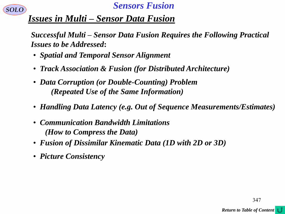
347
Sensors FusionSOLO
Issues in Multi – Sensor Data Fusion
Successful Multi – Sensor Data Fusion Requires the Following Practical
Issues to be Addressed:
• Spatial and Temporal Sensor Alignment
• Track Association & Fusion (for Distributed Architecture)
• Data Corruption (or Double-Counting) Problem
(Repeated Use of the Same Information)
• Handling Data Latency (e.g. Out of Sequence Measurements/Estimates)
• Communication Bandwidth Limitations
(How to Compress the Data)
• Fusion of Dissimilar Kinematic Data (1D with 2D or 3D)
• Picture Consistency
Return to Table of Content

348
Multi Target TrackingSOLO
References
S.S. Blackman, “Multiple-Target Tracking with Radar Applications”, Artech House, 1986
S.S. Blackman, R. Popoli , “Design and Analysis of Modern Tracking Systems”,
Artech House, 1999
Y. Bar-Shalom, T.E. Fortmann, “Tracking and Data Association”, Academic Press, 1988
E. Waltz, J. Llinas, “Multisensor Data Fusion”, Artech House, 1990
Y. Bar-Shalom, Ed., “Multitarget-Multisensor Tracking, Applications and Advances”,
Vol. II, Artech House, 1992
Y. Bar-Shalom, Xiao-Rong Li., “Multitarget-Multisensor Tracking: Principles and
Techniques”, YBS Publishing, 1995
Y. Bar-Shalom, W.D. Blair,“Multitarget-Multisensor Tracking, Applications and Advances”,
Vol. III, Artech House, 2000
Y. Bar-Shalom, Ed., “Multitarget-Multisensor Tracking, Applications and Advances”,
Vol. I, Artech House, 1990
Y. Bar-Shalom, Xiao-Rong Li., “Estimation and Tracking: Principles, Techniques
and Software”, Artech House, 1993
L.D.Stone, C.A. Barlow, T.L. Corwin, “Bayesian Multiple Target Tracking”,
Artech House, 1999

349
Multi Target TrackingSOLO
References (continue – 1)
Ristik, B. & Hernanadez, M.L., “Tracking Systems”, 2008 IEEE Radar Conference,
Rome, Italy
Return to Table of Content
Karlsson, R., “Simulation Based Methods for Target Tracking”,
Linköping University, Thesis No. 930, 2002
Karlsson, R., “Particle Filtering for Positioning and Tracking Applications”,
PhD Dissertation, Linköping University, No. 924, 2005

350
Multi Target TrackingSOLO
References
S.S. Blackman, “Multiple-Target Tracking with Radar Applications”, Artech House, 1986
S.S. Blackman, R. Popoli “Design and Analysis of Modern Tracking Systems”,
Artech House, 1999
L.A. Klein, “Sensor and Data Fusion”, Artech House,

351
Multi Target TrackingSOLO
References
D. Hall, J. Llinas,“Handbook of Multisensor Data Fusion”, Artech House,
D. Hall, S. A. H. McMullen, “Mathematical Techniques in Multisensor Data Fusion”.
Artech House
M.E. Liggins, D. Hall, J. Llinas, Ed.“Handbook of Multisensor Data Fusion:
Theory and Practice”, 2nd Ed., CRC Press, 2008

352
Multi Target TrackingSOLO
References
Y. Bar-Shalom, Ed.,“Multitarget-Multisensor Tracking, Applications and Advances”,
Vol. II, Artech House, 1992
Y. Bar-Shalom, W.D. Blair Ed.,“Multitarget-Multisensor Tracking, Applications and
Advances”, Vol. III, Artech House,
L.D.Stone, C.A. Barlow, T.L. Corwin, “Bayesian Multiple Target Tracking”,
Artech House, 1999

353
Multi Target TrackingSOLO
References
From left-to-right: Sam Blackman, Oliver Drummond,
Yaakoov Bar-Shalom and Rabinder MadanFrom left-to-right: Fred Daum, X. Rong Li, Tom Kerr and
Sanjeev Arulambalam
A Raytheon THAAD radar, which uses Yaakov’s Bar-Shalom
JPDAF algorithm
httf://esplab1.ee.uconn.edu/AESmagMae02.htm The Workshop on Estimation, Tracking and Fusion:
A Tribute to Yaakov Bar-Shalom, 17 May 2001
354
Multi Target TrackingSOLO
References
“Special Issue in Data Fusion”, Proceedings of the IEEE, January 1997
Klein, L. A., “Sensor and Data Fusion Concepts and Applications”, 2nd Ed.,
SPIE Optical Engineering Press, 1999
355“Proceedings of the IEEE”, March 2004, Special Issue on:
“Sequential State Estimation: From Kalman Filters to Particle Filters”
Julier, S.,J. and Uhlmann, J.,K., “Unscented Filtering and Nonlinear Estimation”,
pp.401 - 422

356
Branko Ristic Marcel L. Hernandez
Fredrik Gustafsson Niclas Bergman Rickard Karlsson

357
SOLO
Technion
Israeli Institute of Technology
1964 – 1968 BSc EE
1968 – 1971 MSc EE
Israeli Air Force
1970 – 1974
RAFAEL
Israeli Armament Development Authority
1974 – 2013
Stanford University
1983 – 1986 PhD AA
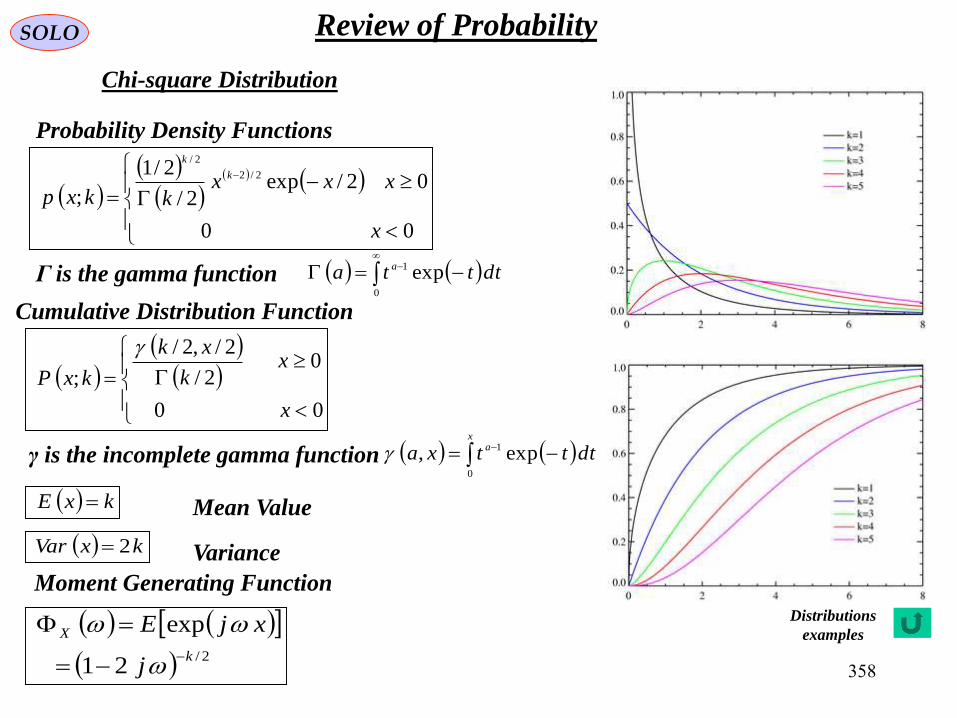
358
SOLO Review of Probability
Chi-square Distribution
00
02/exp2/
2/1
;
2/2
2/
x
xxxkkxp
k
k
kxE
kxVar 2
2/21
exp
k
X
j
xjE
Probability Density Functions
Cumulative Distribution Function
Mean Value
Variance
Moment Generating Function
00
02/
2/,2/
;
x
xk
xk
kxP
Γ is the gamma function
0
1 exp dttta a
x
a dtttxa0
1 exp,γ is the incomplete gamma function
Distributions
examples
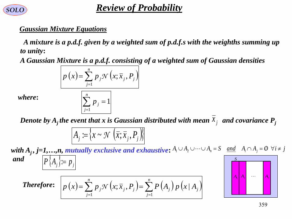
359
SOLO Review of Probability
Gaussian Mixture Equations
A mixture is a p.d.f. given by a weighted sum of p.d.f.s with the weighths summing up
to unity:
n
j
jjj Pxxpxp1
,;N
A Gaussian Mixture is a p.d.f. consisting of a weighted sum of Gaussian densities
where:1
1
n
j
jp
jjj PxxxA ,;~: N
Denote by Aj the event that x is Gaussian distributed with mean and covariance Pjjx
with Aj , j=1,…,n, mutually exclusive and exhaustive:
and S
1A 2A nA
jj pAP :
jiOAAandSAAA jin 21
n
j
jj
n
j
jjj AxpAPPxxpxp11
|,;NTherefore:

360
SOLO Review of Probability
Gaussian Mixture Equations (continue – 1)
A Gaussian Mixture is a p.d.f. consisting of a weighted sum of Gaussian densities
n
j
jj
n
j
jjj AxpAPPxxpxp11
|,;N
The mean of such a mixture is:
n
j
jj
n
j
jjj xpPxxEpxpxEx11
,;N
The covariance of the mixture is:
n
j
j
T
jj
n
j
jj
T
jj
n
j
j
T
jjj
n
j
jj
T
jj
n
j
jj
T
jjjj
n
j
jj
TT
pxxxxpAxxExx
pxxAxxEpAxxxxE
pAxxxxxxxxE
pAxxxxExxxxE
110
10
1
1
1

361
SOLO Review of Probability
Gaussian Mixture Equations (continue – 2)
The covariance of the mixture is:
PpPpxxxxpAxxxxExxxxEn
j
jj
n
j
j
T
jj
n
j
jj
T
jj
T ~
111
where:
n
j
j
T
jj pxxxxP1
:~
Is the spread of the mean term.
Tn
j
j
T
jj
n
j
j
TT
x
n
j
jj
x
n
j
j
T
j
n
j
j
T
jj
xxpxx
pxxxpxpxxpxxP
T
1
1
1111
:~
Tn
j
j
T
jj
n
j
jj
TxxpxxpPxxxxE
11
Note: Since we developed only first and second moments of the mixture, those relations
will still be correct even if the random variables in the mixture are not Gaussian.

362
SOLO Probability
Total Probability Theorem
Table of Content
nAAAS 21
jiOAA ji
1A2A
nAB
jiOAAandSAAA jin 21If
we say that the set space S is decomposed in exhaustive and
incompatible (exclusive) sets.
The Total Probability Theorem states that for any event B,
its probability can be decomposed in terms of conditional
probability as follows:
n
i
i
n
i
i BPBABAB11
|Pr,PrPr
Using the relation:
llll AABBBABA Pr|PrPr|PrPr
klOBABABAB lk
n
k
k ,1
n
k
k BAB1
PrPr
For any event B
we obtain:

363
SOLO Probability
Statistical Independent Events
n
i
i
n
n
kjikji i
i
n
jiji i
i
n
i
i
tIndependenlStatisticaA
n
i
i
n
n
kjikji
kji
n
jiji
ji
n
i
i
n
i
i
AAAA
AAAAAAAA
i
1
13
,.
3
1
2
.
2
1
1
1
1
13
,.
2
.
1
11
Pr1PrPrPr
Pr1PrPrPrPr
From Theorem of Addition
Therefore
n
i
i
tIndependenlStatisticaA
n
i
i AA
i
11
Pr1Pr1
n
i
i
tIndependenlStatisticaA
n
i
i AA
i
11
Pr11Pr
Since OAASAAn
i
i
n
i
i
n
i
i
n
i
i
1111
&
n
i
i
n
i
i AA11
PrPr1
n
i
i
tIndependenlStatisticaA
n
i
i AA
i
11
PrPr If the n events Ai i = 1,2,…n are statistical independent
than are also statistical independentiA
n
i
iA1
Pr
n
i
i
MorganDe
A1
Pr
n
i
i
tIndependenlStatisticaA
A
i
1
Pr1
nrAAr
i
i
r
i
i ,,2PrPr11
Table of Content

364
SOLO Probability
Theorem of Multiplication
12112312121 |Pr|Pr|PrPrPr AAAAAAAAAAAAA nnn
Proof
ABABA /PrPrPr Start from
12121 /PrPrPr AAAAAAA nn
2131212 /Pr/Pr/Pr AAAAAAAAA nn
in the same way
12122112211 /Pr/Pr/Pr nnnnnnn AAAAAAAAAAAAA
From those results we obtain:
12112312121 |Pr|Pr|PrPrPr AAAAAAAAAAAAA nnn
q.e.d.
Table of Content
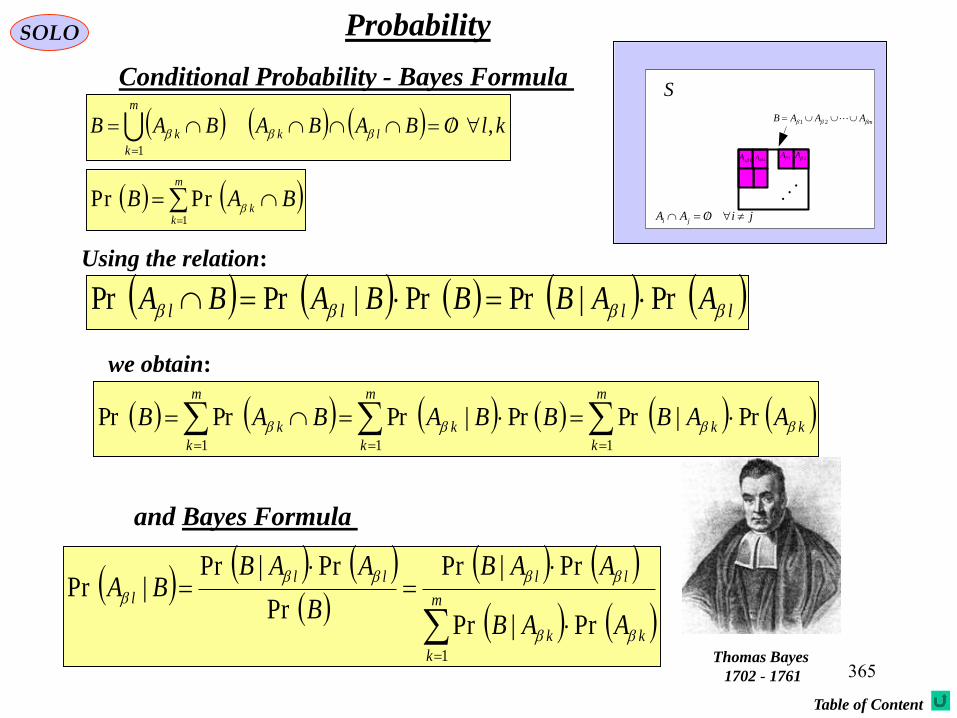
365
SOLO Probability
Conditional Probability - Bayes Formula
Using the relation:
llll AABBBABA Pr|PrPr|PrPr
klOBABABAB lk
m
k
k ,1
m
kk
BAB1
PrPr
we obtain:
m
k
kk
llll
l
AAB
AAB
B
AABBA
1
Pr|Pr
Pr|Pr
Pr
Pr|Pr|Pr
and Bayes Formula
Thomas Bayes
1702 - 1761
S
jiOAA ji
1A
mAAAB 21
2A 1A 2A
Table of Content
m
k
kk
m
k
k
m
k
k AABBBABAB111
Pr|PrPr|PrPrPr