1 Time Synchronizationand Calibrationin Wireless Sensor Networks

Kay Romer, Philipp Blum, Lennart Meier

ETH Zurich, Switzerland

In this chapter, we review time synchronization and calibration for wireless sensornetworks. We will first consider time synchronization in Sections 1.1–1.6, beforeturning to calibration in Section 1.7. We will show that time synchronization can beconsidered as a calibration problem and many observations about time synchroniza-tion can be transferred to calibration.

In Section 1.1, we discuss applications of synchronized time in sensor networks,present challenges of sensor networks, and discuss why traditional synchronizationapproaches fail to meet these challenges. Section 1.2 presents models of sensornodes, of hardware clocks, and of communication. Section 1.3 gives an overviewof the various classes of synchronization. In Section 1.4, we present common syn-chronization techniques. Section 1.5 examines current synchronization algorithms.Section 1.6 presents common techniques for evaluating synchronization algorithmsand selected evaluation results.

1.1 INTRODUCTION

Sensor networks are used to monitor real-world phenomena. For such monitoringapplications, physical time often plays a crucial role. We will discuss these applica-tions of time in Section 1.1.1. Providing synchronized physical time is a complextask due to various challenging characteristics of sensor networks. In Section 1.1.2,we present these challenges and discuss why synchronization algorithms for tradi-tional distributed systems often do not meet these challenges.

i

ii

(a)

(b)

(c)

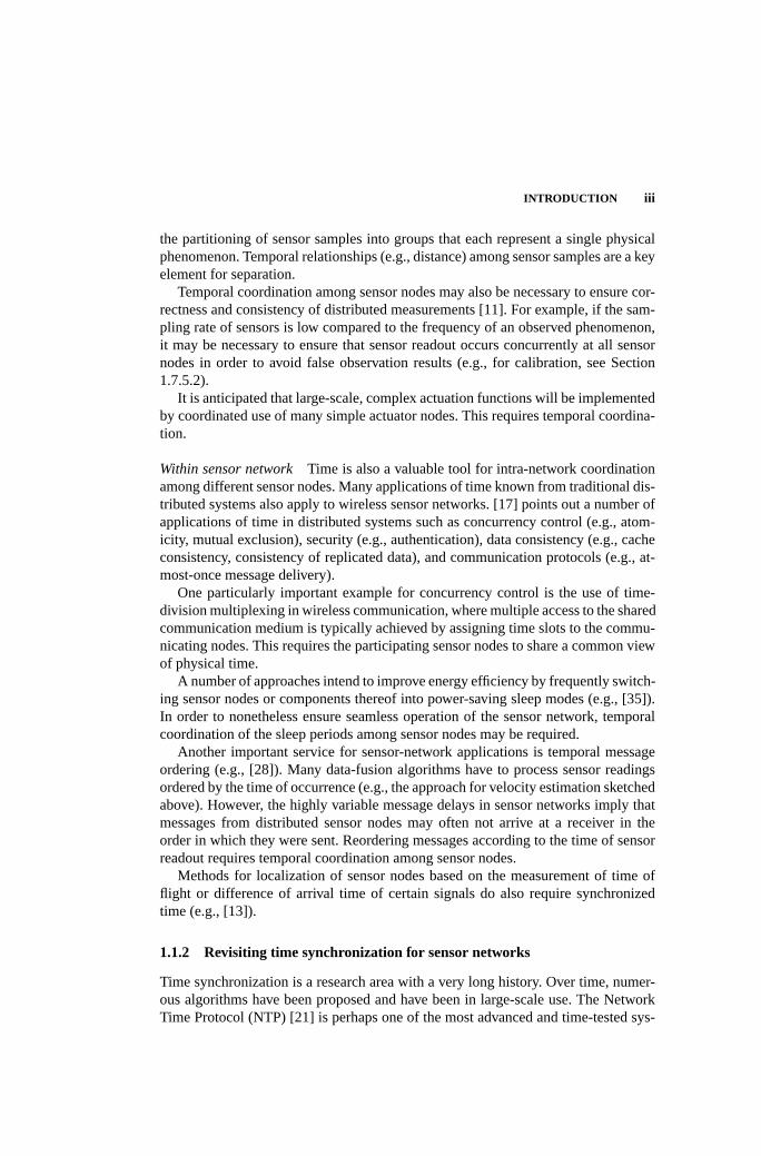
Fig. 1.1 Applications of physical time: (a) interaction of an external observer with the sensornetwork, (b) interaction among sensor nodes, and (c) interaction of the sensor network withthe real world.

1.1.1 The need for synchronized time

Physical time plays a crucial role for many sensor-network applications. While manytraditional applications of time also apply to sensor networks, we will focus here onareas specific to sensor networks. Figure 1.1 illustrates a rough classification of ap-plications of physical time: (a) at the interface between the sensor network and anexternal observer, (b) among the nodes of the sensor network, and (c) at the inter-face between the sensor network and the observed physical world. The followingparagraphs will discuss applications of time in these three domains. Note that someapplications are hard to assign to a single domain. In such cases, we picked the mostappropriate domain.

Sensor network – observerIn many applications, a sensor network interfaces toan external observer for tasking, reporting results, and management. This observermay be a human operator or an autonomous computing system. Tasking a sensornetwork often involves the specification of time windows of interest such as “onlyduring the night”. As a sensor network reports observation results to an externalobserver, temporal properties of observed physical phenomena may be of interest.For example, the times of occurrence of physical events are often crucial for theobserver to associate event reports with the originating physical events. Physical timeis also crucial for determining properties such as speed or acceleration.

Sensor network – real world In sensor networks, many sensor nodes may observe asingle physical phenomenon. One of the key functions of a sensor network is hencethe assembly of those distributed observations into a coherent estimate of the originalphenomenon — this process is known as data fusion. Time is a key ingredient fordata fusion. For example, if sensors can only detect the proximity of an object, thenhigher-level information (such as speed, size, or shape) can be obtained by correlat-ing data from multiple sensor nodes. The velocity of a mobile object, for example,can be estimated by the quotient of the spatial and temporal distances between twoconsecutive sightings of the object by different sensor nodes.

Since many instances of a physical phenomenon can occur within a short time,one of the tasks of a sensor network is the separation of sensor samples, that is

INTRODUCTION iii

the partitioning of sensor samples into groups that each represent a single physicalphenomenon. Temporal relationships (e.g., distance) among sensor samples are a keyelement for separation.

Temporal coordination among sensor nodes may also be necessary to ensure cor-rectness and consistency of distributed measurements [11]. For example, if the sam-pling rate of sensors is low compared to the frequency of an observed phenomenon,it may be necessary to ensure that sensor readout occurs concurrently at all sensornodes in order to avoid false observation results (e.g., for calibration, see Section1.7.5.2).

It is anticipated that large-scale, complex actuation functions will be implementedby coordinated use of many simple actuator nodes. This requires temporal coordina-tion.

Within sensor network Time is also a valuable tool for intra-network coordinationamong different sensor nodes. Many applications of time known from traditional dis-tributed systems also apply to wireless sensor networks. [17] points out a number ofapplications of time in distributed systems such as concurrency control (e.g., atom-icity, mutual exclusion), security (e.g., authentication), data consistency (e.g., cacheconsistency, consistency of replicated data), and communication protocols (e.g., at-most-once message delivery).

One particularly important example for concurrency control is the use of time-division multiplexing in wireless communication, where multiple access to the sharedcommunication medium is typically achieved by assigning time slots to the commu-nicating nodes. This requires the participating sensor nodes to share a common viewof physical time.

A number of approaches intend to improve energy efficiency by frequently switch-ing sensor nodes or components thereof into power-saving sleep modes (e.g., [35]).In order to nonetheless ensure seamless operation of the sensor network, temporalcoordination of the sleep periods among sensor nodes may be required.

Another important service for sensor-network applications is temporal messageordering (e.g., [28]). Many data-fusion algorithms have to process sensor readingsordered by the time of occurrence (e.g., the approach for velocity estimation sketchedabove). However, the highly variable message delays in sensor networks imply thatmessages from distributed sensor nodes may often not arrive at a receiver in theorder in which they were sent. Reordering messages according to the time of sensorreadout requires temporal coordination among sensor nodes.

Methods for localization of sensor nodes based on the measurement of time offlight or difference of arrival time of certain signals do also require synchronizedtime (e.g., [13]).

1.1.2 Revisiting time synchronization for sensor networks

Time synchronization is a research area with a very long history. Over time, numer-ous algorithms have been proposed and have been in large-scale use. The NetworkTime Protocol (NTP) [21] is perhaps one of the most advanced and time-tested sys-

iv

tems. However, several unique characteristics of sensor networks often preclude theuse of existing synchronization techniques in this domain.

In the following, we discuss sensor-network challenges that impact the design oftime-synchronization approaches. Using NTP as an example, we will outline whytraditional approaches often do not meet the requirements of sensor networks (seealso [9]). Note that some of the illustrated shortcomings of NTP are relatively easyto fix, while others are not. To provide the necessary background, we will first givean overview of NTP.

NTP was designed for large-scale networks with a rather static topology (such asthe Internet). Nodes are externally synchronized to a global reference time that isinjected into the network at many places via a set of master nodes (so-called “stra-tum 1” servers). These master nodes are synchronized out of band, for example viaGPS (which provides global time with a precision significantly below 1µs). Nodesparticipating in NTP form a hierarchy: leaf nodes are called clients, inner nodes arecalled stratumL servers, whereL is the level of the node in the hierarchy. The parentsof each node must be specified in configuration files at each node. Nodes frequentlyexchange synchronization messages with their parents and use the obtained informa-tion to adjust their clocks by regularly incrementing them.

Energy and other resourcesSensor-network applications often require sensor nodesto be small and cheap. This has a number of important implications. First of all, theamount of energy that can be stored in or scavenged by small devices is typicallyvery limited due to the low energy density of available and foreseeable technology.To ensure longevity despite this limited energy budget, energy-efficient design bothin hardware and software becomes a dominating goal. Additionally, computing, stor-age, and communication capabilities of individual sensor nodes are rather limited dueto size and energy constraints.

These constraints may preclude the use of GPS or other technologies for out-of-band synchronization of NTP master nodes. NTP is also not optimized for energyefficiency, simply because this is not an issue in infrastructure-based distributed sys-tems. Energy overhead in NTP results from several sources. Firstly, the service pro-vided by NTP typically cannot be dynamically adapted to the varying needs of anapplication. Hence, with NTP all nodes would be continuously synchronized withmaximum precision, even though only subsets of nodes might occasionally needsynchronized time with less-than-maximum precision.

Secondly, NTP uses the processor and the network in ways that would lead tosignificant overhead in energy expenditure in sensor networks. For example, NTPmaintains a synchronized system clock by regularly adding small increments to thesystem-clock counter. This behavior precludes the processor from being switched toa power-saving idle mode. In addition, NTP servers must be prepared to receive syn-chronization requests at any point in time. However, constantly listening is an energy-wise costly operation in sensor networks; many sensor-network protocols thereforeswitch off the radio whenever possible.

INTRODUCTION v

Network dynamics Due to their deployment in the physical environment, sensornetworks are subject to a high degree of network dynamics. Sensor nodes can bemobile, die due to depleted batteries or due to environmental influences, and newsensor nodes may be added at any point in time. This results in relatively frequentand unpredictable changes in the network topology and possibly even in (temporary)network partitions. Mobile nodes can transport messages across partition boundariesby storing a received message and forwarding it as soon as a new partition is entered.The end-to-end delay of such message paths is very unstable and hard to predict.

The operation of NTP is independent of the underlying physical network topol-ogy. In the NTP overlay hierarchy, a master and a client can be separated by manyhops in the physical network, even though they are neighbors in the overlay hierar-chy. Due to the above mentioned effects, multi-hop paths may be very unstable andunpredictable in a sensor network. NTP, however, depends on the ability to accu-rately estimate the delay characteristics of network links.

NTP implicitly assumes that network nodes that shall be synchronized are a prioriconnected by the network. However, this assumption may not hold in dynamic sen-sor networks with mobile nodes. Consider for example an application where mobilesensor nodes with sporadic network connectivity time-stamp sensor readings and de-liver these records to an observer as they pass by a base station (e.g., [15]). The basestation may then want to compare time stamps generated by different sensor nodesin order to evaluate the collected data. However, in the above scenario, there mightnot be a network connection between the various originators of the time-stampedmessages at any point in time. Hence, NTP cannot be applied in such settings.

Infrastructure In many applications, sensor networks have to be deployed in re-mote, unexploited, or hostile regions. Sensor networks therefore often cannot relyon sophisticated hardware infrastructure. For example, under dense foliage or insidebuildings, GPS cannot be used since there is no free line of sight to the GPS satellites.

In order to improve the precision and availability of synchronization in large net-works, NTP injects the reference time at many points into the network. Hence, anynode in the network is likely to find a source of reference time in a distance of onlya few hops. Note that shorter paths tend to be more reliable and more predictable,since they include fewer sources of error and unpredictability.

However, such an approach requires an external infrastructure of reference-timesources which have to be synchronized with some out-of-band mechanism. Wherethis is not feasible, NTP would have to operate with a single master node, whichuses its local time as the reference time. In large sensor networks, the average pathlength from a node to this single master is long, leading to reduced precision. This isparticularly problematic when collocated sensor nodes require very precise mutualsynchronization, for example to cooperate in observing a nearby physical event. Witha single master node, the collocated nodes might end up using different synchroniza-tion paths, which results in different synchronization errors (i.e., time offsets) withrespect to the master node.

vi

Configuration After initial deployment, it is often infeasible to physically accessthe sensor nodes for hardware or software maintenance. The large number of nodesalso precludes manual configuration of individual nodes. While traditional networkssuch as the Internet do also consist of a large number of nodes, there is an accordinglylarge number of human network administrators, such that each one takes care of amanageable number of computers. With sensor networks, however, half a dozen ofhuman operators may be responsible for thousands of sensor nodes.

NTP requires the specification of one or more potential synchronization mastersfor each node. This is an appropriate solution for networks with a rather static topol-ogy, where configurations remain valid for extended periods of time. In sensor net-works, however, network dynamics necessitate a frequent adaptation of configurationparameters.

1.2 SYSTEM MODEL

In the sections ahead we will analyze various synchronization approaches. We willnow specify the system model for time synchronization that we use as the founda-tion of our analysis. First, we describe how we model clocks. We then specify thecharacteristics of communication between nodes in a sensor network.

All our modeling is done in terms of discrete time and events. An event can rep-resent communication between nodes, a sensor measurement, the injection of timeinformation at a node, etc. We denote the real time at which eventa occurs asta, andthe local time of nodeNi at that time ashi

a. Note that our model does not explicitlycontain node mobility or network dynamics; these aspects are included implicitly bythe absence or existence of corresponding communication events.

1.2.1 Clock models

Digital clocks measure time intervals. They typically consist of a counterh (whichwe will also refer to as “the (local) clock”) that counts time steps of an ideally fixedlength; we denote the reading of the counter at real timet ash(t). The counter isincremented by an oscillator with a rate (or frequency)f . The rate f at time t isgiven as the first derivative ofh(t): f (t) = dh(t)/dt. An ideal clock would have rate1 at all times, but the rate of a real clock fluctuates over time due to changes insupply voltage, temperature, etc. If the fluctuation were allowed to be arbitrary, theclock’s reading would obviously give no information at all. Fortunately, it is limitedby known bounds. Different types of bounds on the rate fluctuation lead to differentclock models:

Constant-rate model The rate is assumed to be constant. This is reasonable if therequired precision is small compared to the rate fluctuation.

SYSTEM MODEL vii

Bounded-drift model The deviation of the rate from the standard rate 1 is assumedto be bounded. We call this deviation the clock’sdrift ρ(t) = f (t)−1= dh(t)/dt−1,and denote the corresponding bound withρmax:

−ρmax≤ ρ(t)≤ ρmax ∀t . (1.1)

A reasonable additional assumption isρi(t) >−1 for all timest. This means that aclock can never stop (ρi(t) =−1) or run backward (ρi(t) <−1). Thus, if two eventsa, b with ta < tb occur at a nodeNi whose clock’s driftρi is bounded according to(1.1), then nodeNi can compute lower and upper bounds∆l

i [a,b], ∆ui [a,b] on the

real-time difference∆[a,b] := tb− ta as:

∆li [a,b] :=

hi(tb)−hi(ta)1+ρmax

∆ui [a,b] :=

hi(tb)−hi(ta)1−ρmax

. (1.2)

This model is typically reasonable, since bounds on the oscillator’s rate are givenby the hardware manufacturer. Sensor nodes usually contain non-expensive oscilla-tors, and thus we haveρmax∈ [10 ppm,100 ppm]1. Note that in this model, the driftcan jump arbitrarily within the bounds specified in (1.1). The next model limits thevariation of the drift.

Bounded-drift-variation model The variationϑ(t) = dρ(t)/dt of the clock drift isassumed to be bounded:

−ϑmax≤ ϑ(t)≤ ϑmax ∀t . (1.3)

This assumption is reasonable if the drift is influenced only by gradually chang-ing conditions such as temperature or battery voltage. It makes drift compensationpossible: A node can estimate its current drift and compute bounds on its drift forfuture times.

We can also assume both (1.1) and (1.3).

1.2.2 Software clocks

A synchronization algorithm can either directly modify the local clockh or otherwiseconstruct a software clockc. A software clock is a function taking a local clock valueh(t) as input and transforming it to the timec(h(t)). This time is the final resultof synchronization, and we therefore call it the synchronized time. For example,c(h(t)) = t0 +h(t)−h(t0) is a software clock that starts with the correct real timet0and then runs with the same speed as the local clockh. In general, we require that asoftware clock is a piecewise continuous, strictly monotonically increasing function.

1Parts per million, that is 10−6. A clock with a drift of 100 ppm drifts 100 seconds in a million seconds,or 100µs in one second.

viii

1.2.3 Communication models

Communication is needed to obtain and maintain synchronization. In the following,we identify different communication parameters that affect time synchronization.

Unicast vs. multicast If a message is sent by one network node and is received byat most one other network node, we call this unicast or point-to-point communica-tion. Multicast communication occurs when a message is sent by one network nodeand is received by an arbitrary number of other network nodes. The case where allnodes within transmission range are recipients is called broadcast. Wireless sensornetworks typically use simple broadcast radios, such that a sensor node’s transmis-sion is overheard by all nodes within its transmission range.

Symmetrical vs. asymmetrical linksIf we assume that nodeA can receive messagessent by nodeB if and only if nodeB can receive messages sent by nodeA, we saythat the link between these two nodes is symmetrical. Otherwise, it is asymmetrical.An example for an asymmetrical link is the link between a base station with hightransmit power and a mobile device with low transmit power: Beyond a certain dis-tance between the two, only communication in direction from the base station to themobile device is possible. In wireless sensor networks, it is reasonable to assume thatthere is a large number of small sensor nodes, and a small number of more powerful(regarding energy, memory, processing power, and transmit power) nodes. The linksbetween these two types of nodes would clearly be asymmetrical.

Implicit vs. explicit synchronizationWhen comparing clock-synchronization ap-proaches, it is important to distinguish whether synchronization information can besent only with the messages that the sensor-network application transmits (“piggy-back”), or whether additional communication (i.e., messages sent only for the sakeof synchronization) is allowed. There is a trade-off between the amount of additionalcommunication and the achievable synchronization quality. Additional communica-tion incurs additional energy consumption and can reduce the bandwidth availablefor application data. Piggy-backed time information does typically not reduce band-width significantly, since there are no additional message headers to be transmittedor transmission slots to be occupied, and the time information is small in size.

Delay uncertainty As far as synchronization is concerned, the goal of communica-tion is to convey time information. The delay of the messages sent between nodeshas to be taken into account when extracting this time information; we will explorethis in Section 1.4.1. The message delay consists of

• the send time, lasting from when the application issues the send command towhen the node actually starts trying to send; it is caused by kernel processing,context switches, and system calls, and hence varies with the current systemload,

SYSTEM MODEL ix

• the (medium) access time, lasting from when the node is ready to send towhen it actually starts the transmission; this is the time that is spent waitingfor access to the wireless channel, and hence depends on the current networkload,

• the propagation time, which is the time it takes for the radio signal to travelfrom the sender to the receiver; it is constant for any pair of nodes with constantdistance, and is negligible compared to the other delay components in wirelesssensor networks (since distances are small and radio signals travel very fast),and

• the receive time, lasting from the reception of the signal to the arrival of thedata at the application.

The send and receive time (and especially the uncertainty about them) can be re-duced by implementing the time-stamping of outgoing and incoming messages ata very low level, for instance in the MAC layer. As a general rule, message-delayuncertainties in typical wireless sensor networks are rather large compared to thosein wired networks. This is due to the lower link reliability and bandwidth (see Sec-tion 1.1.2).

1.2.4 Sources of synchronization errors

Clock-synchronization algorithms face two problems: The information a node hasabout the local time of another node degrades over time due to clock drift (the twoclocks “drift apart”), and its improvement through communication is hindered bymessage-delay uncertainty.

The influence of drift and delay uncertainty on the quality of synchronization canto a large extent be studied separately. The influence of the clock drift may dominateover that of the message delays. This is the case in those sensor networks wherecommunication isinfrequent. The reason for this is that with decreasing frequencyof communication, the uncertainty due to clock drift increases, while the uncertaintydue to message delays remains constant.A numeric example:Suppose the messagedelay contributes 1 millisecond to a node’s uncertainty, and the clock drift is boundedby ρmax= 10 ppm. After 50 seconds, the drift’s contribution to the uncertainty equalsthat of the delay. After one hour, it is 72 times larger. In this setting, neglecting thedelay uncertainty is acceptable.

The time information that is obtained through communication has to be processedto achieve synchronization. As we will show in Sections 1.4.1 and 1.4.2, the com-putation power and memory size required to do this in a timely fashion can increase(even nonlinearly) with the amount of communication and thus become very large.There is a trade-off between computational power and storage capacity spent andachievable synchronization.

x

1.3 CLASSES OF SYNCHRONIZATION

Synchronization is commonly understood as “making clocks show the same time”,but there are actually many different types of synchronization. In the following, wewill give an overview of the various choices available for synchronization. Whenchoosing the synchronization approach for a given sensor-network application, themaxim is to fulfill the application’s requirements with the smallest possible effort interms of computation, memory, and especially energy.

1.3.1 Internal vs. external

The synchronization of all clocks in the network to a time supplied from outside thenetwork is referred to asexternalsynchronization. NTP performs external synchro-nization, and so do sensor nodes synchronizing their clocks to a master node. Notethat it makes no difference whether the source of the common system time is also anode in the network or not.

Internalsynchronization is the synchronization of all clocks in the network, with-out a predetermined master time. The only goal here is consistency among the net-work nodes. External synchronization requires consistency within the networkandwith respect to the externally provided system time.

In everyday life, we are mostly faced with external synchronization, namely withkeeping wristwatches and clocks in computers, cell phones, PDAs, cars, microwaveovens, etc. synchronized to the legal time.

1.3.2 Lifetime: continuous vs. on-demand

Thelifetimeof synchronization is the period of time during which synchronization isrequired to hold. If time synchronization iscontinuous, the network nodes strive tomaintain synchronization (of a given quality) at all times. For some sensor-networkapplications,on-demandsynchronization can be as good as continuous synchroniza-tion in terms of synchronization quality, but much more efficient. During the (pos-sibly long) periods of time between events, no synchronization is needed, and com-munication and hence energy consumption can be kept at a minimum. As the timeintervals between successive events become shorter, a break-even point is reachedwhere continuous and on-demand synchronization perform equally well. There aretwo kinds of on-demand synchronization:

Event-triggeredon-demand synchronization is based on the idea that in order totime-stamp a sensor event, a sensor node needs a synchronized clock only immedi-ately after the event has occurred. It can then compute the time-stamp for the momentin the recent past when the event occurred. Post-facto synchronization [8] is an ex-ample for event-triggered synchronization.

We usetime-triggeredon-demand synchronization if we are interested in obtain-ing sensor data from multiple sensor nodes for a specific time. This means that thereis no event that triggers the sensor nodes, but the nodes have to take a sample atprecisely the right time. This can be achieved viaimmediatesynchronization (where

CLASSES OF SYNCHRONIZATION xi

sensor nodes receive the order to immediately take a sample and time-stamp it) oranticipatedsynchronization (where the order is to take the sample at some futuretime, thetarget time). Anticipated synchronization is necessary if it cannot be guar-anteed that the order can be transmitted rapidly and simultaneously to all involvedsensor nodes. This is especially the case if sensor nodes are more than one hop awayfrom the node giving the order.

Note that for successful anticipated synchronization, it is sufficient to maintaina synchronization quality which guarantees that the target time is not missed. Thismeans that the required synchronization quality grows as the real time approachesthe target time. There is no need to synchronize with maximum quality right fromthe beginning.

Analogously to the event-triggered post-facto synchronization, we might refer totime-triggered synchronization as pre-facto synchronization.

N3

N5

N4

N2

N1

a) b)

Space

Time

N3

N5

N4

N2

N1

Scope

Life

time

Scope

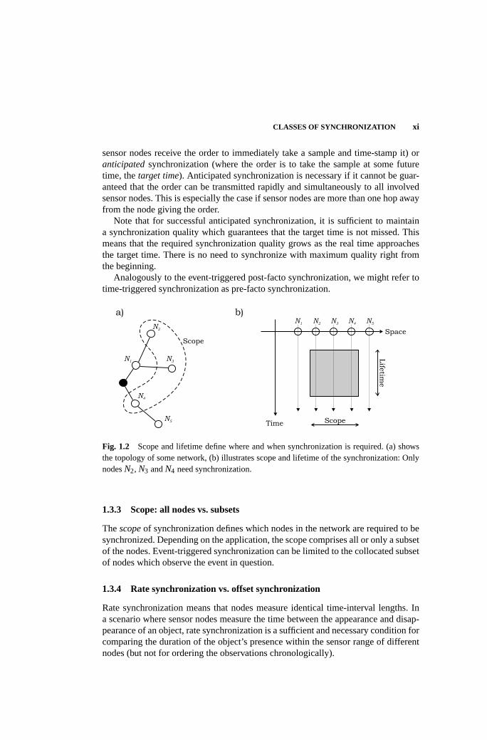
Fig. 1.2 Scope and lifetime define where and when synchronization is required. (a) showsthe topology of some network, (b) illustrates scope and lifetime of the synchronization: OnlynodesN2, N3 andN4 need synchronization.

1.3.3 Scope: all nodes vs. subsets

Thescopeof synchronization defines which nodes in the network are required to besynchronized. Depending on the application, the scope comprises all or only a subsetof the nodes. Event-triggered synchronization can be limited to the collocated subsetof nodes which observe the event in question.

1.3.4 Rate synchronization vs. offset synchronization

Rate synchronization means that nodes measure identical time-interval lengths. Ina scenario where sensor nodes measure the time between the appearance and disap-pearance of an object, rate synchronization is a sufficient and necessary condition forcomparing the duration of the object’s presence within the sensor range of differentnodes (but not for ordering the observations chronologically).

xii

Offset synchronization means that nodes measure identical points in time, that isat some timet, the software clocks of all nodes in the scope showt. Offset synchro-nization is needed for combining time stamps from different nodes.

The difference between rate and offset synchronization is illustrated in Figure 1.3.NodeN2 can compute the bird’s speed all by itself by dividing the distance betweenthe bird’s positions at eventsa andb by the corresponding local-time difference. Forthis, the node’s clock must be rate-synchronized to the real-time rate 1. Alternatively,data from nodesN2 andN3 can be combined to compute the bird’s speed; here, wewould use eventsb andc. The nodes’ clocks have to be offset-synchronized for this.

cN

3

N2 N

1

a

b

Fig. 1.3 At eventsa, b, andc, nodesN2 andN3 measure the position of the bird and time-stamp this data with their current local time. Rate or offset synchronization is needed dependingon how the data from the three events is to be combined.

1.3.5 Timescale transformation vs. clock synchronization

Time synchronization can be achieved in two fundamentally different ways. We cansynchronize clocks, that is make all clocks display the same time at any given mo-ment. To achieve this, we have to perform rate and offset synchronization (or contin-uous offset synchronization, which however is costly in terms of energy and band-width and requires reliable communication links). The other approach is to transformtimescales, that is to transform local times of one node into local times of anothernode.

Both approaches are equal in the sense that if we have either perfect clock syn-chronization or perfect timescale transformation, the distributed sensor data can becombined as if it had been collected by a single node. The approaches differ inthat clock synchronization requires either communication across the whole network(for internal synchronization) or some degree of global coordination (for externalsynchronization). This calls for communication over multiple hops (which howevertends to degrade synchronization quality), or well-distributed infrastructure whichfor instance guarantees that every sensor node is only a few hops away from a nodeequipped with a GPS receiver. Timescale transformation does not have these draw-backs, but may instead incur additional computation and memory overhead.

We illustrate the difference between clock synchronization and timescale trans-formation using the example shown in Figure 1.3. If the clocks of all three nodes aresynchronized, nodeN1 can directly combine the sensor data from nodesN2 andN3,

SYNCHRONIZATION TECHNIQUES xiii

since the time stamps refer to the same timescale. If the clocks are not synchronized,a timescale transformation on the received time stamps is necessary. The final resultis identical to that of using synchronized clocks.

1.3.6 Time instants vs. time intervals

Time information can be given by specifying time instants (e.g., “t = 5”) or time in-tervals (“t ∈ [4.5,5.5]”). In both cases, the time information can be refined by addinga statement about its quality. For instance, the time information may be guaranteedto be correct with a certain probability, or even probability distributions for the timecan be given. A measure for the quality of the time information can then be defined;we will speak of its inverse, thetime uncertainty.

For sensor networks, the use of guaranteed time intervals can be very attractive.Interestingly, this approach has not received much attention, although it has a numberof advantages over using time instants: (i) Guaranteed bounds on the local times atwhich sensor events occurred allow to obtain guaranteed bounds from sensor-data fu-sion. (ii) The concerted action (sensing, actuating, communicating) of several nodesat a predetermined time always succeeds: each node can minimize its uptime whileguaranteeing its activity at the predetermined time. (iii) The combination of severalbounds for a single local time is unambiguous and optimal, while the reasonablecombination of time estimates requires additional information about the quality ofthe estimates.

1.4 SYNCHRONIZATION TECHNIQUES

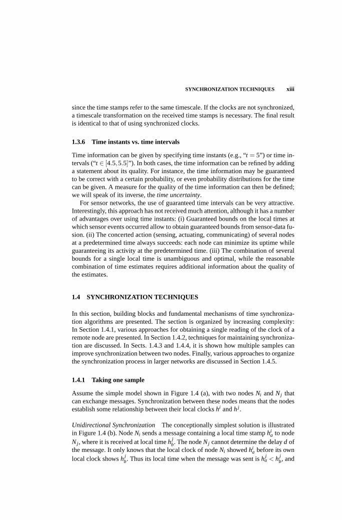
In this section, building blocks and fundamental mechanisms of time synchroniza-tion algorithms are presented. The section is organized by increasing complexity:In Section 1.4.1, various approaches for obtaining a single reading of the clock of aremote node are presented. In Section 1.4.2, techniques for maintaining synchroniza-tion are discussed. In Sects. 1.4.3 and 1.4.4, it is shown how multiple samples canimprove synchronization between two nodes. Finally, various approaches to organizethe synchronization process in larger networks are discussed in Section 1.4.5.

1.4.1 Taking one sample

Assume the simple model shown in Figure 1.4 (a), with two nodesNi andNj thatcan exchange messages. Synchronization between these nodes means that the nodesestablish some relationship between their local clockshi andh j .

Unidirectional Synchronization The conceptionally simplest solution is illustratedin Figure 1.4 (b). NodeNi sends a message containing a local time stamphi

a to nodeNj , where it is received at local timeh j

b. The nodeNj cannot determine the delayd ofthe message. It only knows that the local clock of nodeNi showedhi

a before its ownlocal clock showsh j

b. Thus its local time when the message was sent ish ja < h j

b, and

xiv

a)

Nj

Ni

c)

hi

hj

D

Ni Nj

d

d'

b)

hi

hj

Ni Nj

ha

i

d

d)

hi

hj

Dj

Ni Nj

Di

d '1

d2

d1

d '2

hb

i

ha

j

hb

i

hc

ihb

j

ha

j

hc

j

Fig. 1.4 Uni- and bidirectional synchronization.a) A nodeNj determines the offset ofits local clock relative to that of another nodeNi , b) using unidirectional communication or c)and d) using bidirectional communication. In contrast to c), scheme d) allows both nodes tomeasure a round-trip time.

nodeNi ’s local time when the message is received ishib > hi

a. Time synchronization

consists of estimating eitherhib or h j

a.If a-priori bounds on the message delay are known, that isdmin ≤ d≤ dmax, then

the estimationh ja ≈ h j

b− 1/2(dmin + dmax) (or alternativelyhib ≈ hi

a + 1/2(dmin +dmax)) minimizes the synchronization error in the worst case. Alternatively,h j

b−dmax

andh jb− dmin are lower and upper bounds onh j

a (andhia + dmin andhi

a + dmax arebounds onhi

b).

Round-Trip SynchronizationA slightly more complex solution is illustrated in Fig-ure 1.4 (c). NodeNj sends a query message to nodeNi , asking for the time stamphi

b. NodeNj measures the round-trip timeD = h jc−h j

a, that is the length of the timeinterval between sending the request and receiving the reply. Without having a-prioriknowledge, nodeNj now knows that the delayd is bounded by 0 andD. If a-prioribounds on the message delay are known, that isdmin ≤ d≤ dmax, the nodeNj knowsthatd is bounded by max(D−dmax,dmin) and min(dmax,D−dmin).

The estimationh jb ≈ h j

c−D/2 minimizes the worst-case synchronization error;

h jc− (D−dmin) andh j

c−dmin are lower and upper bounds onh jb. Similarly, an esti-

mation and bounds forhic can be determined.

In comparison with the unidirectional approach, round-trip synchronization hasthe advantage of providing an upper bound on the synchronization error. The mech-anism known asprobabilistic time synchronization first presented in [5] uses this todecrease the synchronization error as follows: After receiving the reply message,Nj

checks whether the worst-case synchronization errorD/2−dmin is below a specifiedthreshold. If not, it sends a new request message toNi . This procedure is repeateduntil a pair of request and reply messages occurs that achieves the required syn-chronization error. The smaller the chosen threshold, the more messages have to beexchanged on average.

SYNCHRONIZATION TECHNIQUES xv

The main disadvantage of round-trip synchronization is that the amount of mes-sages increases linearly with the number of nodes that communicate withNi , while inthe unidirectional case, a single broadcast message sent byNi can serve an arbitrarynumber of nodes. A combination of the advantages of both approaches is knownaseavesdroppingor anonymous synchronizationand was first described in [7]. Thebasic idea is the following: NodeNj sends a broadcast message toNi and some addi-tional nodeNk, Ni replies with a broadcast message toNj andNk. NodeNk assumesthat the second message was produced after it had received the first message, thusnodeNk can do round-trip synchronization with the two local receive time stampsand the send time stamp fromNi without ever producing any messages itself.

In Figure 1.4 (d), two modifications of round-trip synchronization are illustrated.Firstly, it is not necessary thatNi replies immediately to query messages. NodeNi caninstead measure the durationDi between receiving the query message and sendingthe reply, and the nodeNj can then account for this duration in its calculations.Secondly, the message exchange shown in Figure 1.4 (c) is asymmetrical, that isonlyNj can do round-trip synchronization. Therefore, at least one additional messagefrom Nj to Ni is required, such that alsoNi can estimate or bound remote time stamps.

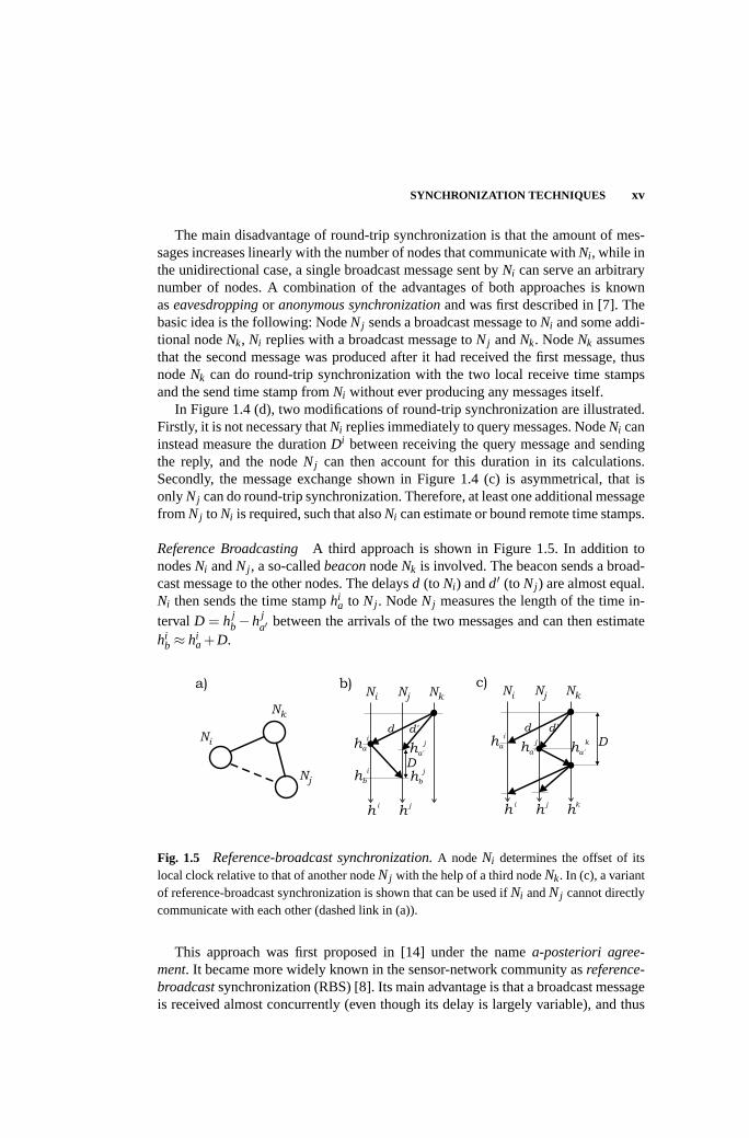
Reference BroadcastingA third approach is shown in Figure 1.5. In addition tonodesNi andNj , a so-calledbeaconnodeNk is involved. The beacon sends a broad-cast message to the other nodes. The delaysd (to Ni) andd′ (to Nj ) are almost equal.Ni then sends the time stamphi

a to Nj . NodeNj measures the length of the time in-tervalD = h j

b−h ja′ between the arrivals of the two messages and can then estimate

hib ≈ hi

a +D.

Nk

D

a) c)

d d'

Nj

Ni

Ni NkNj

hi

hk

D

b)

d d'

Ni NkNj

ha

i

hi

hj h

j

hb

i

ha'

j

hb

j

ha

i

ha'

kha'

j

Fig. 1.5 Reference-broadcast synchronization.A nodeNi determines the offset of itslocal clock relative to that of another nodeNj with the help of a third nodeNk. In (c), a variantof reference-broadcast synchronization is shown that can be used ifNi andNj cannot directlycommunicate with each other (dashed link in (a)).

This approach was first proposed in [14] under the namea-posteriori agree-ment. It became more widely known in the sensor-network community asreference-broadcastsynchronization (RBS) [8]. Its main advantage is that a broadcast messageis received almost concurrently (even though its delay is largely variable), and thus

xvi

the synchronization error typically is smaller than with unidirectional or round-tripsynchronization.

The reference-broadcast technique can be used in many variations. For example,Figure 1.5 (c) shows a solution presented in [6] for the case that nodesNi andNj ,while being able to receive messages fromNk, cannot communicate with each otherdirectly.Nj replies toNk, which then can estimate its own local timehk

a′ and send thisinformation in another broadcast message toNi andNj . In [8], yet another version isdescribed: All nodes report their time stamps to a single node, which then broadcastsall information.

The disadvantage of the reference broadcast approach is that physical broadcastsand a beacon node are required.

1.4.2 Synchronization in rounds

Typically, two local clocks do not run at exactly the same speed. Therefore time syn-chronization has to be refreshed periodically, the duration of the round dependingon the error budget and the amount of relative drift between the two clocks. Let thelength of a round beτround. Assume a round consists of a first period with lengthτsample, where one or more samples are taken according to one of the methods de-scribed in Section 1.4.1, and a second period where the nodes do nothing. Let usassume, that an application allows for a total error ofEtotal, the maximum error aftertaking the samples isEsample, and the maximal drift rate isρmax. Then the maximumlength of a roundτround has to satisfy

τround≤Etotal−Esample

ρmax.

The above relation implies that rounds can be longer ifEsampleandρmaxare small. Forexample, algorithms that use the round-trip technique can boundEsampleaccording tothe measured round-trip time and thus can dynamically increaseτround if the round-trip time was small. Other algorithms compensate the drift of the local clock andtherefore can compute a smaller effectiveρmax, which also allows to increaseτround.

In some applications,Etotal is smaller than what can be guaranteed by taking asingle sample. In such a case, multiple samples can be taken to achieveEsample<Etotal. Taking multiple samples increasesτsample. At the limit, τsample≈ τround; in thiscase, synchronization in rounds becomes a continuous process, rounds follow eachother seamlessly.

1.4.3 Combining multiple time estimates

We now discuss techniques for combining multiple estimates of the local time of aremote node. Figure 1.6 (a) illustrates the situation: Every circle stands for a singleestimate of nodeN j ’s local timeh j

a at some eventa, which occurs atNi ’s local timehi

a.

SYNCHRONIZATION TECHNIQUES xvii

hi

hj

hi

hj

a) b)

Fig. 1.6 Multiple samples improve on the synchronization error.(a) Every point rep-resents a sample, that is a local timehi of nodeNi and an estimated local timeh j of nodeNj .Using interpolation techniques improves on the synchronization error. The solid line resultsfrom a linear regression on the samples, the dashed line is the result of a phase-locked loop(PLL). (b) The same idea can be used for lower (5) and upper (4) bounds on the local timeof Nj . Also here, interpolation can considerably improve on the synchronization error (i.e., onthe uncertainty in this case). The solid lines are determined by the convex-hull approach, thedashed lines according to [30].

Linear Regression The most widely used technique is linear regression. A linearrelation h j = α + β · hi is postulated and the coefficientsα and β are determinedby minimizing the square of the difference between the fittedh j ’s and the actualsamples. This technique has a single parameter, that is the number of samples thatare accounted for when computing the coefficients. A large number of samples canimprove the regression quality, but requires a large amount of memory.

The coefficientβ can be interpreted as an estimation ofh j ’s drift relative tohi .Linear regression thus implicitly compensates for clock drift. If the drift is variable,the postulated linear relationship betweenh j andhi does not describe reality verywell. In such a situation, the number of samples accounted for should be small.

The linear regression can be computed on-line, that is incrementally whenever anew sample is taken. An efficient on-line implementation can be found in [26]. Adisadvantage of the linear-regression technique is that it weighs data points by thesquare of their error against the fitted line. Outliers thus have a particularly stronginfluence on the resulting coefficientsα andβ.

Phase-Locked LoopsAnother method for processing a continuous sequence ofsamples is based on the principle of phase-locked loops (PLL) [12]. The PLL con-trols the slope of the interpolation using a proportional-integral (PI) controller. Theoutput of a PI controller is the sum of a component that is proportional to the inputand a component that is proportional to the integral of the input. The input of thecontroller is the difference between the actual sample and the interpolated value. If

xviii

the interpolation is smaller than the sample, its slope is increased, otherwise it is de-creased. The main advantage of the PLL-based approach is that it requires far lessmemory than the linear-regression technique (in essence only the current state of theintegrator sum). The main disadvantage is that PLLs require a long convergence timeto achieve a stable rate [25]. The NTP algorithm uses a PLL [22].

1.4.4 Combining multiple time intervals

The techniques of Section 1.4.1 can also be used to derive lower and upper bounds onthe local time of a remote node. Figure 1.6 (b) shows a sequence of lower and upperbounds on the local timesh j of a remote nodeNj on the y-axis and the correspondinglocal timeshi of a nodeNi on the x-axis. In the previous section, the samples formeda single cloud and the interpolation was a line “through the middle of this cloud”.Here we have two clouds, one formed by the lower-bound samples, the other by theupper-bound samples.

The convex-hulltechnique [1, 36] interpolates the two clouds separately. Onecurve is drawn above all lower bounds, a second below all upper bounds. Whilelinear-regression and PLL techniques tend towards the average of the individual sam-ples, the convex-hull technique ignores average values and account for the sampleswith minimal or maximal error. This can result in improved robustness: While thecurrent average message delay can be very unstable, the minimal message delay re-mains stable, though it may occur more or less frequently.

In [30], it is proposed to interpolate lower- and upper-bound samples by a singleline as follows: First the steepest and flattest lines that do not violate any lower orupper bound are determined. The slopes of these lines represent bounds on the driftof clock h j relative tohi . The “average”-line of these two extremal solutions is usedas the final interpolation; for a more detailed description see Section 1.5.3.

1.4.5 Synchronization of multiple nodes

Sensor networks most often have a much more complicated topology than the simpleexamples shown in Figures 1.4 and 1.5, and not all sensor nodes can communicatewith each other directly. Thus, multi-hop synchronization is required, which adds anadditional layer of complexity. Clearly, this could be avoided by using an overlay net-work which provides virtual, single-hop communication from every sensor node to asingle master node. But as we have seen in Section 1.4.1, the synchronization errordirectly depends on the message delay, which is very difficult to control on a logicallink that is composed of many physical hops. Therefore, performant synchronizationschemes have to deal with the multi-hop problem explicitly.

Figure 1.7 illustrates various approaches to multi-hop synchronization. We nowdescribe these four schemes and use them as examples to discuss the main problemsof multi-hop synchronization.

Out-of-band synchronizationThe conceptionally simplest solution is to avoid theproblem: A large number of master nodes is distributed in the network such that every

SYNCHRONIZATION TECHNIQUES xix

a) b) c) d)

Fig. 1.7 Organizing synchronization in multi-hop networks.a) Single-hop synchro-nization with a set of master nodes which are synchronized out of band (e.g., using GPS). b)Single-hop synchronization in overlapping clusters, gateway nodes translate time stamps. c)Tree hierarchy with a single master node at the root. d) Unstructured.

node has a direct connection to at least one of these masters (e.g., [33]). The masternodes are synchronized among each other using some out-of-band mechanism. Theglobal positioning system (GPS) is well suited to this purpose as it provides timeinformation with sub-microsecond accuracy. However, GPS receivers are still rela-tively costly, consume a considerable amount of energy, and require a direct line ofsight to a number of satellites and thus cannot operate inside buildings.

Clustering The authors of the RBS algorithm propose to partition the network intoclusters [8]. All nodes within a cluster can broadcast messages to all other membersof the cluster and thus the reference-broadcast technique can be used to synchronizethe cluster internally. Some nodes are members of several clusters and participateindependently in all corresponding synchronization procedures. These nodes act astime gateways to translate time stamps from one cluster to the other. There is a trade-off in choosing the size of the clusters. On the one hand, a small number of largeclusters reduces the number of translations and thus improves the synchronizationerror; on the other hand, energy consumption grows quickly with increasing trans-mission range; this makes choosing many small clusters attractive. This trade-off hasbeen examined in [23].

Tree Construction The most common solution of the multi-hop synchronizationproblem is to construct a synchronization tree with a single master at the root [10,30, 32, 18]. Single-hop synchronization is applied along the edges of the tree. Vari-ous well-known algorithms can be used to construct such a tree [32]. As the accuracydegrades with the hop distance from the root, a tree with minimum depth is prefer-able. On the other hand, a small depth implies that the root has to serve many clients,and thus consumes far more energy than the other nodes.

Tree construction faces two main problems: Firstly, in sensor networks, the net-work topology may be dynamic; nodes may be mobile and repeatedly join or leavethe network. The multi-hop synchronization algorithms have to explicitly deal withsuch events. In particular, if the root node fails, a new root has to be elected [18].Secondly, two neighboring (in terms of physical location) nodes may have a large

xx

hop distance in the synchronization tree. In consequence, the accuracy of synchro-nization between these nodes is not as good as if they would synchronize directlywith each other.

Unstructured As illustrated in the tree-construction approach, the multi-hop syn-chronization problem can be interpreted as the problem of determining the linksand directions over which time information is disseminated. In contrast to tree-construction approaches,unstructuredapproaches do not first explicitly solve thisproblem and then perform pairwise synchronization. Instead, time information is ex-changed between any pair (or group) of nodes that communicate. Whereas in thetree-construction approach every pairwise synchronization is asymmetrical (i.e., be-tween a client and a local master), it is symmetrical in the unstructured approach (i.e.,between two equal peers). In [2], such an approach has been presented for interval-based synchronization. Two nodes combine their bounds on real time by selectingthe larger lower bound and the smaller upper bound. A similar approach for point-estimates isasynchronous diffusionproposed in [16]. Here, nodes that communicateadjust their synchronized clocks to the average of their synchronized times. Likethe interval-based solution from [2], this approach is completely local. As these ap-proaches do not maintain any global configuration, node mobility does not causeparticular problems. In contrast, clustering and tree-construction schemes requirethat the global configuration has to be updated whenever nodes move or fail or whennew nodes are added to the system.

As algorithms that follow the unstructured approach do not attempt to communi-cate with a particular node (e.g., the parent node in a synchronization tree), some ofthese algorithms piggyback time stamps on messages that are sent for some other,not synchronization-related reason (e.g., [27, 2]). It could be argued that these al-gorithms have virtually no communication overhead, as no messages are generatedexclusively for time synchronization.

1.5 CASE STUDIES

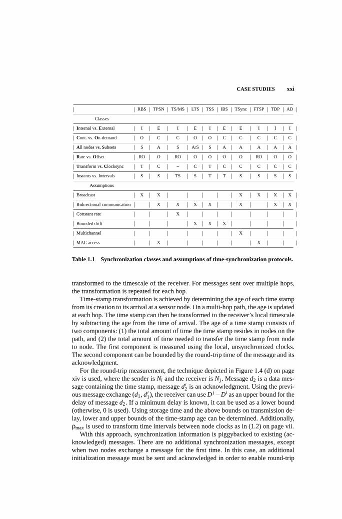
In the following subsections, we discuss a number of concrete synchronization algo-rithms from the literature (ordered by publication date). The goal here is to give anoverview of the approaches (with reference to the techniques and classes discussedearlier in this chapter), rather than to discuss all the details. In addition, for each algo-rithm we will give some experimental results. Table 1.1 summarizes the underlyingassumptions of the various protocols and classifies the approaches according to thecriteria discussed in Section 1.3.

1.5.1 Time-stamp Synchronization (TSS)

TSS [27] provides internal synchronization on demand. Node clocks run unsynchro-nized, that is time stamps are valid only in the node that generated them. However,when a time stamp is sent to another node as part of a message, the time stamp is

CASE STUDIES xxi

RBS TPSN TS/MS LTS TSS IBS TSync FTSP TDP AD

Classes

Internal vs.External I E I E I E E I I I

Cont. vs.On-demand O C C O O C C C C C

All nodes vs.Subsets S A S A/S S A A A A A

Rate vs.Offset RO O RO O O O O RO O O

Transform vs.Clocksync T C – C T C C C C C

Instants vs. Intervals S S TS S T T S S S S

Assumptions

Broadcast X X X X X X

Bidirectional communication X X X X X X X

Constant rate X

Bounded drift X X X

Multichannel X

MAC access X X

Table 1.1 Synchronization classes and assumptions of time-synchronization protocols.

transformed to the timescale of the receiver. For messages sent over multiple hops,the transformation is repeated for each hop.

Time-stamp transformation is achieved by determining the age of each time stampfrom its creation to its arrival at a sensor node. On a multi-hop path, the age is updatedat each hop. The time stamp can then be transformed to the receiver’s local timescaleby subtracting the age from the time of arrival. The age of a time stamp consists oftwo components: (1) the total amount of time the time stamp resides in nodes on thepath, and (2) the total amount of time needed to transfer the time stamp from nodeto node. The first component is measured using the local, unsynchronized clocks.The second component can be bounded by the round-trip time of the message and itsacknowledgment.

For the round-trip measurement, the technique depicted in Figure 1.4 (d) on pagexiv is used, where the sender isNi and the receiver isNj . Messaged2 is a data mes-sage containing the time stamp, messaged′2 is an acknowledgment. Using the previ-ous message exchange (d1, d′1), the receiver can useD j−Di as an upper bound for thedelay of messaged2. If a minimum delay is known, it can be used as a lower bound(otherwise, 0 is used). Using storage time and the above bounds on transmission de-lay, lower and upper bounds of the time-stamp age can be determined. Additionally,ρmax is used to transform time intervals between node clocks as in (1.2) on page vii.

With this approach, synchronization information is piggybacked to existing (ac-knowledged) messages. There are no additional synchronization messages, exceptwhen two nodes exchange a message for the first time. In this case, an additionalinitialization message must be sent and acknowledged in order to enable round-trip

xxii

measurement. An acknowledgment is not needed if the sender can overhear the re-ceiver forwarding the message to the next hop, which is typically the case in broad-cast networks.

Measurements in a wired network withρmax = 1 ppm showed that the averageuncertainty of the time-stamp interval is about 200µs for adjacent nodes. It increasesby an additional 200µs for each additional hop, and by about 2.5µs per age second.

1.5.2 Reference-Broadcast Synchronization (RBS)

RBS [8] provides synchronization for a whole network. The basic synchronizationprimitive is a reference broadcast to a set of client nodes in the one-hop neighbor-hood of a beacon node as illustrated in Figure 1.5 (b) on page xv. The beacon nodebroadcasts manage synchronization pulses. The clients then exchange their respec-tive reception times and use linear regression to compute relative offsets and ratedifferences to each other. Using offset and rate difference, each client can transforma local clock reading to the local timescale of any other client.

To extend this scheme to multi-hop networks, the network is clustered such that asingle beacon can synchronize all nodes in its cluster. Gateway nodes that participatein two or more clusters independently take part in the reference-broadcast procedureof all their clusters. By knowing offsets and rate differences to nodes in all adjacentclusters, gateway nodes can transform time stamps from one cluster to another.

Time synchronization across multiple hops is then provided as follows. Nodestime-stamp sensor data using their local clocks. Whenever time stamps are exchangedamong nodes, the time stamps are transformed to the receiver’s local time using off-set and rate difference.

In experiments it has been shown that adjacent Berkeley Motes can be synchro-nized with an average error of 11µs by using 30 broadcasts. Over multiple hops, theaverage error grows withO(

√n), wheren is the number of hops.

1.5.3 Tiny-Sync and Mini-Sync (TS/MS)

Tiny-Sync and Mini-Sync [30] are methods for pairwise synchronization of sensornodes. Both Tiny-Sync and Mini-Sync use multiple round-trip measurements anda line-fitting technique to obtain the offset and rate difference of the two nodes.For this, a constant-rate model (see page vi) is assumed. To obtain data points forline fitting, multiple round-trip synchronizations are performed as depicted in Figure1.4 (c) on page xiv, where the client isNj and the reference isNi . Each round-tripmeasurement results in a data point(hi

b, [hja,h

jc]). Then, the line-fitting technique

depicted in Figure 1.6 (b) on page xvii is used to calculate two lines with minimumand maximum slope. Slope and axis intercept of these two lines then give bounds forthe relative offset and rate difference of the two nodes. The line with average slopeand intercept of the two lines is then used as the offset and rate difference betweenthe two nodes.

Note that each of the two lines is unambiguously defined by two (a priori un-known) data points. The same results would be obtained if the remaining data points

CASE STUDIES xxiii

could be eliminated. Since the computational and memory overhead depends on thenumber of data points, it is a good idea to remove as many data points as possi-ble before the line fitting. Tiny-Sync and Mini-Sync only differ in this eliminationstep. Essentially, Tiny-Sync uses a heuristic to keep only two data points for each ofthe two lines. However, the selected points may not be the optimal ones. Mini-Syncuses a more complex approach to eliminate exactly those points that do not changethe solution. Hence, Tiny-Sync achieves a slightly suboptimal solution with minimaloverhead, Mini-Sync gives an optimal solution with increased overhead.

Measurements on a 802.11b network with 5000 data points resulted in an offsetbound of 945µs (3230µs) and a rate bound of 0.27 ppm (1.1 ppm) for adjacent nodes(nodes five hops away).

1.5.4 Lightweight Time Synchronization (LTS)

LTS [32] is a synchronization technique that provides a specified precision with littleoverhead, rather than striving for maximum precision as many other techniques.

Two algorithms are proposed: one that operates on demand for nodes that ac-tually need synchronization, and one that proactively synchronizes all nodes. Bothalgorithms assume the existence of one or more master nodes that are synchronizedout-of-band to a reference time. The proactive algorithm proceeds by constructingspanning trees with the masters at the root by flooding the network. In a secondphase, nodes synchronize to their parent in the tree by means of round-trip synchro-nization. The synchronization frequency is calculated from the requested precision,from the depth of the spanning tree, and from the drift boundρmax.

The on-demand version also assumes the existence of one or more master nodes.When a node needs synchronization, it sends a request to one of the masters usingany routing algorithm (this is not further specified). Then, along the reverse path ofthe request message, nodes synchronize using round-trip measurements. The syn-chronization frequency is calculated as in the proactive version described above. Inorder to reduce synchronization overhead, each node may ask its neighbors for pend-ing synchronization requests. If there are any such requests, the node synchronizeswith the neighbor, rather than executing a multi-hop synchronization with a referencenode.

The overhead of the algorithms was examined in simulations with 500 nodes uni-formly placed in a 120 m× 120 m area, a target precision of 0.5 s, and a durationof 10 hours. The centralized algorithm performed an average of 36 pairwise syn-chronizations per node. The distributed algorithm executed 4–5 synchronizations onaverage per node if 65% of all nodes request synchronization.

1.5.5 Timing-Sync Protocol for Sensor Networks (TPSN)

TPSN [10] provides synchronization for a whole network. First, a node is electedas a synchronization master (details for this are not specified), and a spanning treewith the master at the root is constructed by flooding the network. In a second phase,nodes synchronize to their parent in the tree by means of round-trip synchronization.

xxiv

Synchronization is performed in rounds and initiated by the root root broadcast-ing a synchronization-request message to its children. Each child then performs around-trip measurement to synchronize with the root. Nodes further down in the treeoverhear the messages of their parents and start synchronization when their parentshave synchronized. To eliminate message-delay uncertainties, time-stamping for theround-trip synchronization is done in the MAC layer. In case of node failures andtopology changes, master election and tree construction must be repeated.

Measurements showed that two adjacent Berkeley Motes can be synchronizedwith an average error of 16.9µs, which is a worse figure than the 11µs given forRBS in [8]. However, the authors of [10] claim that a re-implementation of RBSon their hardware resulted in an average error of 29.1µs between adjacent nodes,effectively claiming that TPSN is about twice as precise as RBS.

1.5.6 TSync

TSync [6] provides two protocols for external synchronization: the Hierarchy Ref-erencing Time Synchronization Protocol (HRTS) for proactive synchronization ofthe whole network, and the Individual-Based Time Request Protocol (ITR) for on-demand synchronization of individual nodes. Both protocols use an independent ra-dio channel for synchronization messages in order to avoid inaccuracies due to vari-able delays introduced by packet collisions. In addition, the existence of one or moremaster nodes with access to a reference time is assumed.

With HRTS, a spanning tree with the master at the root is constructed. Then,the master uses the reference broadcasting technique illustrated in Figure 1.5 (c) onpage xv to synchronize its children. Each child node now repeats the procedure forits subtree.

Measurements in a network of MANTIS sensor nodes showed a mean synchro-nization error of 21.2µs (29.5µs) for two adjacent nodes (nodes three hops away).For comparison, RBS was also implemented, giving an average error of 20.3µs (28.9µs).

1.5.7 Interval-Based Synchronization (IBS)

Interval-based synchronization was first proposed in [19], where a bounded-driftmodel (see page vi) is assumed. The network nodes perform external synchronizationby maintaining a lower and upper bound on the current time. During communicationbetween two nodes, the bounds are exchanged and combined by choosing the largerlower and the smaller upper bound. This amounts to intersecting the time intervalsdefined by each pair of bounds. Between communications, each node advances itsbounds according to the elapsed real time and the known drift bounds. In [29], themodel was refined by including bounded drift variation and fault-tolerance.

In [2], the simple approach from [19] was shown to be worst-case-optimal, wherethe worst case is the one where all clocks run with maximal drift. A considerable im-provement in the synchronization quality can be achieved by having each node store,maintain, communicate, and use the bounds from its last communications with other

CASE STUDIES xxv

nodes. In [20], it was shown that optimal interval-based synchronization can only beachieved by having nodes store and communicate their entire history. Obviously, thisbecomes prohibitive with growing network size and lifetime. In realistic settings, thevalue of a piece of history data decreases rapidly with its age. Therefore, efficientaverage-case-optimal synchronization can be obtained by using only recent data.

1.5.8 Flooding Time-Synchronization Protocol (FTSP)

FTSP [18] can be used to synchronize a whole network. The node with the lowestnode ID is elected as a leader that serves as a source of reference time. If this nodefails, then the node with the lowest ID in the remaining network is elected as the newleader. The leader periodically floods the network with a synchronization messagethat contains the leader’s current time. Nodes which have not received this messageyet record the contained time stamp and the time of arrival, and broadcast the mes-sage to their neighbors after updating the time stamp. Time-stamping is performedin the MAC layer to minimize delay variability and hence uncertainty.

Each node collects eight (time stamp, time of arrival) pairs and uses linear regres-sion on these eight data points to estimate offset and rate difference to the leader.

Measurements were performed in an eight-by-eight grid of Berkeley Motes, whereeach Mote has a direct radio link to its eight closest neighbors. With this setup, thenetwork synchronized in 10 minutes to an average (maximum) synchronization errorof 11.7µs (38µs), giving an average error of 1.7µs per hop.

1.5.9 Asynchronous Diffusion (AD)

AD [16] supports the internal synchronization of a whole network. The algorithmis very simple: each node periodically sends a broadcast message to its neighbors,which reply with a message containing their current time. The receiver averages thereceived time stamps and broadcasts the average to the neighbors, which adopt thisvalue as their new time. It is assumed that this sequence of operations is atomic, thatis the averaging operations of the nodes must be properly sequenced.

Simulations with a random network of 200 static nodes showed that the synchro-nization error decreases exponentially with the number of rounds.

1.5.10 Time Diffusion Synchronization (TDP)

TDP [31] supports the synchronization of a whole network. Initially, a set of mas-ter nodes is elected. For external synchronization, these nodes must have access toa global time. This is not required for internal synchronization, where masters areinitially unsynchronized.

Master nodes then broadcast a request message containing their current time, andall receivers send back a reply message. Using these round-trip measurements, amaster node calculates and broadcasts the average message delay and standard devi-ation. Receiving nodes record these data for all leaders. Then, they turn themselvesinto so-called “diffused leaders” and repeat the procedure. The average delays and

xxvi

standard deviations are summed up along the path from the masters. The diffusionprocedure stops at a given number of hops from the masters.

All nodes have now received from one or more mastersm the timehm at the initialleader, the accumulated message delay∆m, and the accumulated standard deviationβm. A clock estimate is computed as∑mωm(hm+∆m), where the weightsωm areinversely proportional to the standard deviationβm. After all nodes have updatedtheir clocks, new masters are elected and the procedure is repeated until all nodeclocks have converged to a common time.

In a simulation with 200 static nodes with 802.11 radios and a delay of 5 sec-onds between consecutive synchronization rounds, the deviation of time across thenetwork dropped to 0.6 seconds after about 200 seconds.

1.6 EVALUATION STRATEGIES

Evaluating the precision of time synchronization in wireless sensor networks is nota trivial task. For example, the authors of the RBS algorithm report 11µs precisionon the Berkeley Motes platform [8], while the authors of the TPSN algorithm report29 µs for RBS on the same platform, concluding that TPSN is better, as it achieves17µs [10]. Which numbers are correct? Probably all of them, but the evaluation wasdone slightly differently.

In this section, we discuss different evaluation strategies that have been appliedto time-synchronization algorithms for wireless sensor networks. There are variousaspects of the performance achieved by an algorithm than can be evaluated, for ex-ample the energy consumption or the message and memory overhead. The discussionin this section concentrates on various alternatives for the evaluation of theprecisionof time-synchronization algorithms.

1.6.1 What is precision?

Figure 1.2 (b) on page xi illustrates the scope and lifetime of synchronization in asensor network. The scope defines which nodes have to be synchronized and thelifetime defines when these nodes have to be synchronized. Thus it is natural toevaluate the precision in the shaded area of Figure 1.2 (b). The precision is a metricthat is closely related to the synchronization error. While the precision is a singlescalar value for a whole network, the synchronization error is a function of time fora single node. In the following, we discuss several alternatives to map such functionsto a single scalar precision valueP.

Combining the synchronization error of many nodesAt some timet within thelifetime of a sensor network, every nodeNi within the scope has a synchronized timeci(hi(t)). In the case of internal synchronization, theinstantaneous precision p(t) is

EVALUATION STRATEGIES xxvii

often defined as the maximal difference between any two synchronized times, that is

p(t) = maxi, j

{ci(hi(t))−c j(h j(t))

}for any nodesNi andNj within the scope. Some authors (e.g., [31]) use the standarddeviation among allci(hi(t)) as a measure for the instantaneous precision at timet.

In the case of external synchronization, the instantaneous precision is more oftendefined as the maximal synchronization error, that is

p(t) = maxi

{ci(hi(t))− t

}for any nodeNi within the scope. This variant of precision is sometimes calledaccu-racy. Alternatively, the precision can be defined as the average synchronization errorwithin the scope or the maximal synchronization error among the 90% (or 99%, etc.)nodes in the scope with the smallest synchronization error.

Steady State and Convergence TimeThe instantaneous precisionp(t) obviouslyvaries during the synchronization lifetime. The final precision metricP can be de-rived by taking the maximum ofp(t) for all t in the lifetime. Alternatively, the aver-age ofp(t) can be used.

It is clear that the precisionP improves in proportion to the time the synchroniza-tion process is active, and that at some point, the improvement stops. Usually, theprecisionP is evaluated after this point, that is the lifetime of synchronization startsafter the synchronization process, and the precisionP describes thesteady state.

Some authors evaluate theconvergence time, which is the length of the intervalfrom the start of the synchronization process to the point in time where the precisionP stops to improve or reaches a specific value. If the lifetime is defined, the conver-gence time indicates when the synchronization process has to be started such that thedesired precisionP is achieved before the start of the lifetime and is maintained untilthe end of the lifetime.

1.6.2 Goals of performance evaluation

There can be different reasons why the performance of an algorithm has to be evalu-ated, and different goals lead to different solutions.

The actual performance of a given synchronization algorithm strongly dependson properties of the target platform. It is difficult to identify and model all the in-fluence factors explicitly. Arealistic estimationof the achievable precision is thusbest obtained by usingmeasurements on the actual target platform, rather than usingsimulation of a simplified target platform.

Sometimes, realistic estimation of the performance is less important thanfairnessand repeatabilityof the evaluation. This is the case if several competing algorithmshave to be compared. Also in the optimization process of the parameters of a partic-ular algorithm, it is important that differences in the performance are due to differ-ences in the algorithm and not due to different conditions (e.g., message delays, clock

xxviii

drift). Here,simulation based on recorded or generated tracesis more appropriatethan direct measurements.

If the goal of analyzing a particular synchronization algorithm is to give worst-case guarantees on its performance, neither measurements nor simulation based onrecorded traces can be used, since both strategies only evaluate a finite number ofinstances. Instead, the worst-case has to be identified and the worst-case performancehas to be determined analytically.

1.6.3 Measurements

Measurement techniquesThree fundamentally different measurement strategies,which are illustrated in Figure 1.8, have been used in recent publications.

LogFile

LogFile

LogFile

LogFileLog

FileAnalyzer

a) b) c)

generate eventsout-of-band synchronization

virtual nodes on asingle physical node

Fig. 1.8 Precision-measurement techniques.a) Every node is synchronized out of bandand measures its own precision. b) Every node generates events, the evaluation is centralized.c) Some nodes are virtual nodes on the same hardware platform as the master node.

Consider Figure 1.8 (a). Every sensor node executes two synchronization proce-dures, synchronizing two different clocks. The first procedure is the actual synchro-nization algorithm under test, using only the means of the platform on which it isexecuted. The second procedure is another algorithm, which achieves a far betterprecision than the first. This is possible since this second synchronization uses re-sources that are not offered by the target platform, but which are introduced for themeasurements. A GPS receiver for every sensor node can serve this purpose. Alter-natively, cable connections can be used as an out-of-band mechanism with very lowdelay variability to provide a reference time (e.g., [24], [8], [3]). In [18], a single-hop RBS scheme is used to measure the precision achieved by the FTSP multi-hopalgorithm. This approach has the advantage that every node can evaluate and log itsown precision and these values can be collected at the end of the experiment (or evenon-line), providing complete information.

An alternative is shown in Figure 1.8 (b). All sensor nodes generate some directlyobservable event, for example a rising edge on a particular I/O pin, when their syn-chronized time reaches a particular valueX. An external analyzer device then recordsthe time interval between the instance when a node’s synchronized time isX and theinstance when it really isX. Such a procedure has been used for example in [10]. Its

EVALUATION STRATEGIES xxix

advantage is that the precision of the measurement is not limited by the resolution ofthe nodes’ clocks or the performance of a second synchronization procedure.

As illustrated in Figure 1.8 (c), [27] proposes to measure the precision achieved byoneclient node as follows: A client node synchronizes over several hops to a masternode. Master and client nodes are virtual nodes emulated on a single physical node,the intermediate nodes are all separate physical nodes. As the master and the clientshare a single hardware clock, the precision of the client can easily be evaluated.

Systems and TopologiesAll three approaches do not scale well. Therefore, onlysmall networks have been used so far for measurements. The largest experiment isdescribed in [18], where a 8-by-7 grid of Mica2 Motes is evaluated. In [10], a chainof 6 Mica Motes is used, [6] evaluates 5 MANTIS Nymph nodes, [27] evaluates achain of 7 standard PCs with 100 Mbit/s wired Ethernet, and [8] evaluates IPAQnodes communicating over 802.11b WLAN and Mica Motes.

How the synchronization error of hundreds of nodes should be measured is anopen question. Current evaluations of such large networks are all based on simula-tion.

Results We will now give some measurement results from recent publications. Ourintention is to give an idea about the order of magnitude of the achievable precisionand to illustrate that although all results are about precision, they are difficult tocompare. In [18], the convergence time of the FTSP algorithm in a 7-by-8 grid isreported to be 10 minutes. A maximal error of 38µs and an average error (over allnodes) of 12µs is reported. For the TPSN algorithm, [10] reports a maximal error of45 µs for one hop and 74µs for five hops. Average errors (over time) are 17µs forone hop and 38µs for five hops. The authors provide also the percentage of the timewhen the synchronization error was below the average error (> 60%). The authors ofRBS present in [8] the distribution of the synchronization error (over time) for onehop and the mean, median, 95% and 99% values over 300 trials for one to four hops.

Some authors evaluate the distribution of the synchronization quality in the sys-tem. At some timet, either the synchronized timesci(hi(t)) of all nodesi [31], oralternatively the corresponding synchronization errorsei(t) [10, 6], are shown in ahistogram.

1.6.4 Simulation

Performance evaluation through simulation has the advantage that the resulting pre-cision or accuracy of all nodes does not have to be measured but is directly accessible.Thus, much larger systems can be evaluated.

Systems and TopologiesIn [31], systems with 200 nodes are evaluated, in [16] and[32] up to 500 nodes, always randomly placed in a square area. The transmissionrange of the nodes is 10 m in a square of length 80 m [31] or 120 m [32]; in [16],various transmission ranges from 0.4 m to 1 m are used in a square of length 10 m.

xxx

In [2], the transmission range is varied between 0.1 and 0.5 times the width of thesquare area. In [30], a chain of 5 nodes is simulated.

Message Delays For simulation, a number of assumptions about the behavior of thesystem have to be made (e.g., about message delays). In [30], measured delay tracesfrom an 802.11 wireless LAN are used, [31] and [32] generate delay traces accordingto a normal distribution. In [31], an additional offset is added which increases whenthe medium is saturated, that is when more than 75% of the channel capacity isused. The authors of [2] assume zero message delay, arguing that the synchronizationerrors induced by delay uncertainty and drift can be studied separately.

Clock Drift In [31] and [2], every node is assigned an arbitrary but constant driftrate between−100 ppm and+100 ppm. In [32], all nodes have a drift rate of 50 ppm.

Results The main concern of [32] is to compare centralized and distributed versionsof the LTS algorithm in terms of required messages and achieved synchronization er-ror. The average error (over all nodes) is evaluated as a function of the hop distance tothe master node. [30] evaluates the synchronization error and the drift-compensationerror achieved by the TS/MS algorithms as a function of time. A node one hop awayfrom the master has an error of 1 ms after 83 minutes. A node with five hops dis-tance achieves 3 ms. In [2], the average synchronization error (over time and over allnodes) is evaluated as a function of the number of messages exchanged between thenodes. Also the impact of the transmission range and of the number of master nodesis evaluated. The authors of [16] mainly evaluate how quickly (number of rounds)a network synchronizes using the AD algorithm. This is evaluated as a function ofthe transmission range and as a function of the number of nodes in the system. Itis also shown that the synchronization error decreases exponentially with the num-ber of rounds. The speed of convergence is also evaluated in [31], here for the TDPand TPSN algorithms; the standard deviation of the nodes’ synchronization erroris shown as a function of time. It is argued that node mobility makes convergenceslower. In addition, histograms and three-dimensional plots of the distribution of thesynchronization error after convergence are presented.

1.6.5 Challenges of a benchmark

So far, we have presented how synchronization algorithms are evaluated in currentliterature. We have seen that results of different authors are quite incomparable dueto widely differing goals, assumptions and techniques. On the one hand, there is notyet a common understanding about the requirements on synchronization in sensornetworks. On the other hand, there is also disagreement about available resourcesand platforms.

A benchmark for comparing the various algorithms on common grounds has notyet been presented. In the following, we discuss why it is difficult to devise a bench-mark that can be used with a large number of algorithms. Ideally, the comparison ofalgorithms is based on simulation using system traces. Such traces should contain

CALIBRATION xxxi

the system and communication model (How many nodes are there? How many ofthem are master nodes? Which node communicates with which other node at whichtime?), and they should characterize the “adversary” of synchronization, namely allmessage delays and the drift rates of the nodes. But this would require to determineall communications before executing the algorithms. This is not possible for most ofthe algorithms, since they actively decide to generate messages, depending on previ-ous events. Furthermore, some algorithms require broadcast communication, whileothers do not.

1.7 CALIBRATION

In the previous sections, we have considered the problem of time synchronization,where the output of a hardware clock had to be mapped to a timescale. Sensor cali-bration is the problem of mapping the output of a sensor to a well-defined scale. Inthis section, we want to take a step back from time synchronization and consider themore general problem of calibration. As we will show, there is a close relationshipbetween calibration and time synchronization, since the latter can be considered aspecial case of the former. It might be somewhat unfamiliar to consider a hardwareclock as a sensor, but we will as show in Section 1.7.1 that the difference is rathersubtle. The remainder of this section is structured in a similar way as the discussionof time synchronization in the previous sections. Section 1.7.2 explains why newapproaches are required for calibration in sensor networks. Section 1.7.3 presentsour system model for sensors. Section 1.7.4 discusses various classes of calibration.Section 1.7.5 presents concrete calibration algorithms from current literature.

1.7.1 Time synchronization as calibration

Sensors are hardware devices that have an input and an output. The input is a certainphysical quantity in the real world, such as temperature, light intensity, acceleration,radio signal strength, etc. The output typically is a variable electrical signal such asa voltage or current. An analog-to-digital converter converts it to a digital number.

A hardware clock typically consists of four components: a physical system thathas a periodic behavior (e.g., an oscillating quartz, decaying Cesium, a pendulum),a sensor that converts the physical phenomenon to an electrical signal, an analog-to-digital converter (e.g., threshold detector) that converts the output of the sensor to aone-bit number, and a counter that counts the number of rising (or falling) edges seenso far in the digital output stream. Hence, a hardware clock contains, among otherthings, a sensorand the physical phenomenon to observe.

Despite this analogy, time as a physical quantity has some unique characteristics.For example, in many practical settings, observed physical quantities have a ratherlimited range of values (e.g., temperature∈ [−30◦C,+30◦C]). Given a bounded rel-ative sensor error (i.e., bounded drift), the absolute measurement error is then alsobounded. However, physical time eventually grows beyond all bounds. Hence, theabsolute error of a software clock is unbounded unless synchronization messages are

xxxii

exchanged. This explains the need for precise drift compensation and for repeatingsynchronization after a certain amount of time.

1.7.2 Revisiting calibration for sensor networks

Calibration is a very old problem, since it is needed for almost all measurement in-struments. Despite this, calibration in sensor networks has so far not received muchattention by researchers — at least when compared to time synchronization. How-ever, a number of challenges to calibration in sensor networks pose interesting ques-tions.

A large number of sensor nodes often cannot be calibrated manually and individ-ually. This is particularly true for pairwise calibration, where a sensor measures aquantity emitted by another device (i.e., an actuator). One example for this is mea-suring the radio signal strength to infer the distance between devices. In such a sce-nario, every sensor would have to be calibrated against every transmitter, resulting ina quadratic number of calibration steps.

Sensors may be exposed to significant changes of environmental parameters (e.g.,temperature, humidity) during the lifetime of a sensor network. Since the commonlyused low-cost sensors are rather sensitive to such changes, a one-time factory cali-bration may not be sufficient. In this case, periodical calibration during the lifetimeof the sensor network is necessary.

1.7.3 System model

The physical quantityq that is observed by a sensor is mainly a function of thesize of the sensor, of its orientation, of its location, and of timet. Since the sizeof a sensor is non-zero, sensors can typically only observe the accumulation (e.g.,weighted average) of a physical quantity over a certain area or volume. If we assumethat size, orientation, and location are constant properties of a sensori, we can denotethe time-dependent physical quantity observed by the sensor asqi(t). Often,q is areal-valued scalar function (e.g., for temperature sensors), but may also be morecomplex (e.g., for a location sensor,q might return triples(x,y,z)).

The output of a sensori under stimulusqi(t) is denoted ashi(t). Note thathi(t) fora givenqi(t) typically depends on a number of parameters, for example fabricationtolerance of the sensor, environmental parameters such as temperature and humidity,and wear of the sensor.

In analogy to software clocks, we introduce asoftware sensoras a functioncthat maps a sensor outputh(t) to c(h(t)). Software sensors are typically introducedto map a sensor output to a standard scale (e.g., the Celsius scale). Here, the goalof calibration is to find a suitablec for a given scale. Often,q does refer to sucha standard scale, in which case the goal of calibration could be to find ac whichapproximatesci(hi(t)) = qi(t) for all t.

As mentioned in the previous section, calibration may also be applied to actuators.An actuator can be considered a reverse sensor that accepts a digital valueh(t) asinput and produces a physical quantityq(t) as output. For example, a heater may

CALIBRATION xxxiii

accept a temperature specification as input and heat until this temperature is reached.A software actuator c−1 then maps a given valuev to c−1(v), which may be usedas an input to the actuator to produce a certain physical quantity (e.g., such thatq(t) = v).

1.7.4 Classes of calibration

In this section, we adapt the classes of time synchronization introduced in Section1.3 to calibration.

Internal vs. external For internal calibration, all software sensorsi should outputthe same valueci(hi(t)) if they are exposed to an identical stimulusq(t) (note that iffor instanceq(t) = 25◦C, thenc1(h1(t)) = c2(h2(t)) = 10◦C would mean that sensors1 and 2 are internally calibrated). For external calibration, the output of all softwaresensors must conform to a specified scale (e.g., ifq(t) = 25◦C, thenc1(h1(t)) =c2(h2(t)) = 25◦C is required).

Lifetime: continuous vs. on-demandAs some of the parameters that influencehmay change over time, calibration may have to be repeated to adapt to these param-eters. Calibration may be performed continuously or on demand.

Scope: all nodes vs. subsetsAll nodes or only subsets of nodes might participatein calibration. For example, only some nodes might be equipped with a certain typeof sensor, or the sensor might only be used by some nodes.

Rate vs. offset Sometimes it is sufficient if differencesci(hi(t1))− ci(hi(t2)) (e.g.,temperature differences) obtained from different sensor instances can be compared.In this case, rate calibration is sufficient. If, however, absolute valuesci(hi(t)) (e.g.,absolute temperature values) originating from different sensor nodes are to be com-pared, offset calibration is needed.

Scale transformation vs. global scaleRather than having all software sensors ad-here to a global scale, it might be advantageous (e.g., in terms of overhead) to main-tain local scales and transform sensor readings as they are sent to nodes with a dif-ferent scale (e.g., if node 1 uses the Celsius scale and node 2 uses the Fahrenheitscale, then the transformation function for transforming from node 1 to node 2 isc12(h1(t)) = 1.8h1(t)+32).

Point estimates vs. boundsSoftware sensors may either output point estimates (inanalogy to time instants for time synchronization) or bounds (in analogy to intervalsfor time synchronization).

xxxiv

1.7.5 Case studies

In this section, we present two calibration algorithms for sensor networks (orderedby publication date). As in Section 1.5, we outline the algorithm and give an idea ofits performance.

1.7.5.1 Calibration as Parameter Estimation (CPE)Calibration as ParameterEstimation [34] provides a framework for external calibration where sensors measurea quantity emitted by an actuator. Both the behavior of the actuator and of the sensorare unknown and must be taken into account for calibration. The general approachhere is the joint calibration of sensors and actuators such that the overall systemresponse is optimized.

The algorithm will be illustrated by pairwise distance measurements between sen-sor nodes using the time of flight of an ultrasound signal. Each node is equipped witha speaker (the actuator) and a microphone (the sensor). Assuming the nodes havesynchronized clocks, one node emits an acoustic signal containing a time stamp, theother receives the acoustic signal, computes the time of flight, and it multiplies withthe speed of sound to obtain a distance estimate.

For our discussion, we will consider a virtual distance sensor that directly out-puts a distance estimateh(t) given the true distance as the physical stimulusq(t).Due to reasons discussed below, distance estimates include various systematic er-rors. Hence, the goal of calibration is to find a functionc that maps the distanceestimateh(t) to the correct distanceq(t).

For CPE,c must now be parameterized, such that it is expressed as a functionof h and of parameters that describe the various error sources. These parameters arerelated to both the sensor and to the actuator. For example, the distanceh(t) outputby the sensor can be expressed in terms of the true distanceq(t) as follows:

h(t) = BT +BR+GTq(t)+GRq(t)

whereBT andBR refer to constant distance offsets caused by startup times for di-aphragm oscillation in the transmitter and in the receiver, respectively;GT andGR

represent the distance-dependent influence of the transmitter volume and of the re-ceiver sensitivity, respectively. Solving forc(h(t)) := q(t) we obtain:

c(h(t)) = (h(t)−BT −BR)/(GT +GR)

Although there is one instance of the above joint-calibration function for every trans-mitter–receiver pair, there is only one set of parameters(BT ,BR,GT ,GR) for each ofthe N nodes. Hence, we can formulate a linear equation system with 4N variables(i.e., the four above parameters for each node) and 4N equations, which requires4N pairs(h(t),c(h(t)) = q(t)) to solve. Alternatively, more samples can be collectedand least-squares optimization can be used to obtain more accurate estimates forthe parameters. Once the parameters(BT ,BR,GT ,GR) for each node are known, thecalibration functions are also known.

CALIBRATION xxxv

The authors performed an experiment with an 8× 4 square grid of Berkeley Moteswith a node distance of 30cm, such that the true distances between pairs of nodes canbe easily calculated. Each node emitted an ultrasound beacon, which allows all othernodes to estimate their distance to the transmitting node. The average error of theuncalibrated distance estimates is 74.6%. With the above calibration procedure, theaverage error could be reduced to 10.1%.

1.7.5.2 Collaborative In-Place Calibration (CIC) CIC [4] supports internal cal-ibration under a number of assumptions: the sensor nodes should be densely de-ployed, sensor orientation should have a negligible impact on the sensor output,spatial frequency of the observed physical quantity should be low, temporal fre-quency of the quantity should be high. Essentially, these assumptions ensure thatcollocated sensor nodes will see very similar stimuliq(t) that change quickly overtime. Additionally, it is assumed thatq, h, c are real-valued, scalar functions. Cal-ibration functionsc are assumed to be linear functions, although the method couldalso be adapted to non-linear functions. The algorithm consists of two phases. In thefirst phase, pairwise calibration among collocated nodes is performed. In the secondphase, calibration among remote nodes is performed.

In the first phase, collocated pairs of nodes are calibrated against each other. Letus assume node 1 has to be calibrated against node 2. Then the goal is to derive a lin-ear calibration functionc12 with c12(h1(t)) = h2(t). Firstly, both sensor nodes recordsensor readingshi(tx), such that both nodes read out the sensor concurrently attx,which requires clock synchronization. The sensor nodes exchange these readings, sothat node 1 obtains a set of data points(tx,h1(tx),h2(tx)). Sincec12 is assumed tobe linear, it can be derived by linear regression from this set of data points. How-ever, even though sensor readout is synchronized, it is possible that the two sensorsperceived different physical stimuliq1(tx) 6= q2(tx) due to their different locations.Hence, such data points have to be eliminated before regression.

For this, confidence values are assigned to the data data points, and the data pointswith low confidence values are eliminated. The confidence values are obtained byshifting a time window with a given size over the set of data points. For each windowposition, the linear correlation coefficientr ∈ [−1,1] for the contained data points iscalculated. The largerr is, the better the data points fall on a line (i.e., the closerq1(tx) andq2(tx) are). If r is positive, then each data point in the window is furtherexamined. If the data point contributes a positive addend tor, then the confidence ofthis data point is increased byr. The initial confidence of each data point is zero.

After this procedure, all data points with a confidence below a certain thresholdvalue are eliminated. With the remaining set, linear regression is performed to derivea linear calibration functionc12. This function is also assigned a confidence thatequals the linear correlation coefficient of the used data points.

Calibration functions for remote nodes are obtained by concatenating multiplecalibration functions for collocated nodes. For example, for two remote nodes 1 and3, the calibration functionsc12 andc23 may be concatenated to give a calibrationfunction c13(h1(t)) = c23(c12(h1(t))). However, there are typically many ways toconstruct a remote calibration function from many local function. Due to inconsis-

xxxvi

tencies it must be expected that for an alternate calibration functionc′13, we havec13(h1(t)) 6= c′13(h1(t)). Hence, the second phase of the algorithm computes moreconsistent non-local calibration functions ˆc.

The algorithm generates a new set of data points and uses linear regression tocompute ˆci j . To obtain the data points, the algorithm enumerates all concatenatedpaths up to a specified maximum length. Thek-th path{ci j

k } is assigned a confidence

r i jk by multiplying the confidences of the path segments. Using a set of random data

valuesxl , the data points are calculated as(xl ,1N ∑k r i j

k ci jk (xl )), whereN is the number

of concatenated pathsci jk .

The accuracy of the derived calibration functions for collocated sensors was mea-sured in an experiment, where 9 Berkeley Motes with temperature sensors wereplaced in a 3× 3 square grid with a node distance of 5cm. A slowly moving hairdryer was used as a heat source. About 70% of the pairwise calibration functionsdeviated by less than 5◦C. More than 10% were off by more than 10◦C.

1.8 SUMMARY

In this chapter, we discussed various aspects of time synchronization and calibrationin sensor networks. We outlined the applications of physical time and discussed whyexisting algorithms for time synchronization have to be revisited. We also presentedcommon classes of and techniques for synchronization, reviewed time-synchroniza-tion algorithms from the literature, and discussed evaluation strategies. Time syn-chronization was identified as a special case of calibration, and many of the observa-tions about time synchronization could be transferred to calibration.

While time synchronization for sensor networks is an established field of research,calibration has not received that much attention yet. However, we expect that calibra-tion becomes a more active field as sensor networks move beyond the lab and smallfield experiments. Unfortunately, calibration is a much more general and complexproblem than time synchronization. Hence, it is likely that research will first focuson more specific calibration problems. An interesting question is, whether techniquesdeveloped for time synchronization can be adapted to calibration problems.

The case studies of time-synchronization algorithms and the discussion of evalu-ation techniques illustrated the very real problem of evaluating and comparing syn-chronization algorithms. Note that these difficulties do also apply to calibration andmany other distributed algorithms. One of the challenges for future research is hencethe development of methods and tools for the evaluation of time synchronization andcalibration in large-scale sensor networks.

Current application-oriented projects (e.g., [15]) indicate that many simplifyingassumptions about sensor networks (e.g., immobile nodes, fixed network topology)may not hold in practice. Hence, future work might have to revisit existing ap-proaches for time synchronization and calibration under updated assumptions.

SUMMARY xxxvii

REFERENCES

1. Jean-Marc Berthaud. Time synchronization over networks using convex clo-sures.IEEE/ACM Transactions on Networking, 8(2):265–277, 2000.

2. Philipp Blum, Lennart Meier, and Lothar Thiele. Improved interval-based clocksynchronization in sensor networks. InThird International Symposium on In-formation Processing in Sensor Networks, pages 349–358, Berkeley, California,USA, April 2004.

3. Philipp Blum and Lothar Thiele. Clock synchronization using packet streams. InDahlia Malkhi, editor,DISC 2002, Brief Announcements, pages 1–8, 2002.

4. Vladimir Bychkovskiy, Seapahn Megerian, Deborah Estrin, and Miodrag Potkon-jak. A Collaborative Approach to In-Place Sensor Calibration. InIPSN, PaloAlto, USA, April 2003.

5. Flaviu Cristian. Probabilistic clock synchronization.Journal of Distributed Com-puting, 3:146–158, 1989.

6. Hui Dai and Richard Han. Tsync: A lightweight bidirectional time synchroniza-tion service for wireless sensor networks.ACM SIGMOBILE Mobile Computingand Communications Review, 8(1):125–139, January 2004.

7. Danny Dolev, Rudiger Reischuk, Ray Strong, and Ed Wimmers. A decentralizedhigh performance time service architecture. Technical Report 95/26, Institute forComputer Science, University of Lubeck, November 1995.

8. Jeremy Elson, Lewis Girod, and Deborah Estrin. Fine-grained network time syn-chronization using reference broadcasts. InFifth Symposium on Operating Sys-tems Design and Implementation (OSDI 2002), December 2002.

9. Jeremy Elson and Kay Romer. Wireless sensor networks: A new regime fortime synchronization. InFirst Workshop on Hot Topics In Networks (HotNets-I),Princeton, New Jersey, October 2002.

10. Saurabh Ganeriwal, Ram Kumar, and Mani B. Srivastava. Timing-sync protocolfor sensor networks. InFirst ACM Conference on Embedded Networked SensorSystems (SenSys), November 2003.

11. Deepak Ganesan, Silvia Ratnasamy, Hanbiao Wang, and Deborah Estrin. Cop-ing with Irregular Spatio-Temporal Sampling in Sensor Networks.SIGCOMMComputer Communication Review, 34(1):125–130, 2004.

12. Floyd M. Gardner.Phaselock Techniques. Wiley, 1979.

13. Lewis Girod, Vladimir Bychkovskiy, Jeremy Elson, and Deborah Estrin. Locat-ing tiny sensors in time and space: A case study. InInternational Conference onComputer Design ICCD, September 2002.

xxxviii

14. Joseph Y. Halpern and Ichiro Suzuki. Clock synchronization and the power ofbroadcasting.Distributed Computing, 5(2):73–82, 1991.

15. Philo Juang, Hidekazu Oki, Yong Wang, Margaret Martonosi, Li-Shiuan Peh,and D. Rubenstein. Energy-Efficient Computing for Wildlife Tracking: DesignTradeoffs and Early Experiences with ZebraNet. InASPLOS X, San Jose, USA,October 2002.

16. Qun Li and Daniela Rus. Global clock synchronization in sensor networks. InIEEE InfoCom, 2004.

17. Barbara Liskov. Practical uses of synchronized clocks in distributed systems. In10th Annual ACM Symposium on Principles of Distributed Computing (PODC’91),pages 1–10, August 1991.

18. M. Maroti, B. Kusy, G. Simon, and A. Ledeczi. The flooding time synchroniza-tion protocol. InSenSys, Baltimore, USA, November 2004.

19. Keith Marzullo and Susan Owicki. Maintaining the time in a distributed system.In Second annual ACM symposium on Principles of distributed computing, pages295–305. ACM Press, 1983.

20. Lennart Meier, Philipp Blum, and Lothar Thiele. Internal synchronization ofdrift-constraint clocks in ad-hoc sensor networks. InFifth ACM InternationalSymposium on Mobile Ad Hoc Networking and Computing, pages 90–97, Tokyo,Japan, May 2004.

21. David L. Mills. Internet time synchronization: The network time protocol.IEEETransactions on Communications, 39(10):1482–1493, October 1991.

22. David L. Mills. Improved algorithms for synchronizing computer network clocks.IEEE/ACM Transactions on Networks, 3(3):245–254, June 1995.

23. Sayan Mitra and Jesse Rabek. Power efficient clustering for clock synchroniza-tion in dynamic multi-hop networks. unpublished,http://theory.lcs.mit.edu/˜mitras/courses/6829/project/finalreport.ps, 2003.

24. Michael Mock, Reiner Frings, Edgar Nett, and Spiro Trikaliotis. Clock synchro-nization in wireless local area networks. In12th Euromicro Conference on RealTime Systems, pages 183–189, June 2000.

25. Raffaele Noro.Synchronization over Packet-Switched Networks: Theory and Ap-plications. PhD thesis, EPFL, Lausanne, Switzerland, 2000.

26. William H. Press, Saul A. Teukolsky, William T. Vetterli, and Brian P. Flannery.Numerical Recipes in C, 2nd Edition. Cambridge University Press, 1992.

27. Kay Romer. Time synchronization in ad hoc networks. InACM Symposium onMobile Ad-Hoc Networking and Computing, October 2001.

xxxix

28. Kay Romer. Temporal message ordering in wireless sensor networks. InIFIPMediterranean Workshop on Ad-Hoc Networks, pages 131–142, June 2003.

29. Ulrich Schmid and Klaus Schossmaier. Interval-based clock synchronization.Real-Time Systems, 12(2):173–228, 1997.

30. Mihail L. Sichitiu and Chanchai Veerarittiphan. Simple, accurate time synchro-nization for wireless sensor networks. InIEEE Wireless Communications andNetworking Conference (WCNC’03), March 2003.

31. Weilian Su and Ian F. Akyildiz. Time-diffusion synchronization protocol for sen-sor networks.IEEE/ACM Transactions on Networking, 2004. To appear.

32. Jana van Greunen and Jan Rabaey. Lightweight time synchronization for sensornetworks. In2nd ACM International Workshop on Wireless Sensor Networks andApplications, pages 11–19, September 2003.

33. Paulo Verissimo, Luis Rodrigues, and Antonio Casimiro. Cesiumspray: a preciseand accurate global time service for large-scale systems.Real-Time Systems,3(12):243–294, 1997.

34. Kamin Whitehouse and David Culler. Calibration as Parameter Estimation inSensor Networks. InWorkshop on Wireless Sensor Networks and Applications(WSNA) 02, Atlanta, USA, September 2002.

35. Wei Ye, John Heidemann, and Deborah Estrin. An energy-efficient mac protocolfor wireless sensor networks. InIEEE Infocom, New York, NY, USA, June 2002.

36. Li Zhang, Zhen Liu, and Cathy Honghui Xia. Clock synchronization algorithmsfor network measurements. InIEEE INFOCOM, 2002.