§ 1. the science of the nervous system - uidaho.edurwells/techdocs/biological signal...

Biological Signal Processing Richard B. Wells

Chapter 1

Introduction, Definitions, and Overview

§ 1. The Science of the Nervous System For centuries humankind has been fascinated by how the brain and the rest of the nervous

system work. Only in the twentieth century did we truly begin to develop the sort of scientific

understanding of this topic detailed enough to permit a quantitative treatment of the many

questions this study raises. Whatever one's philosophy may be over the question of "mind" vs.

"brain" – and there are many diverse opinions on this – the simple fact is that wherever we find

"mind" there also we find "brain." This makes the study of brain, spinal cord, and the peripheral

nervous system arguably the most human, and in some ways the most personal, of scientific

topics.

Wherever we find "mind" we find "brain"; but is the reverse true? Where we find "brain" do

we also find "mind"? This question is presently very problematical. An ant has a brain, but would

one be willing to say an ant has a mind? Until we reach a generally accepted scientific definition

of what is to be meant by "mind," this question is unscientific. An ant exhibits behaviors, and the

relationship of brain and behavior can be studied. Reber's Dictionary of Psychology warns us,

This term [mind], and what it connotes, is the battered offspring of the union of philosophy and psychology. At some deep level we dearly love and cherish it and see behind its surface great potential but, because of our own inadequacies, we continuously abuse it, harshly and abruptly pummeling it for imagined excesses, and occasionally even lock it away in some dark closet where we cannot hear its insistent whines [REBE: 436].

In this book we will not avoid talking about the psychological manifestations of the

phenomenon of human mind, but our primary focus will always be on the science of the nervous

system. Where we introduce psychological concepts, it will be with an emphasis on how

neuroscience treats these questions and on the biological questions science does feel a

competency to address. Our treatment will therefore be mechanistic and functional rather than

metaphysical, and it will be given with due regard to where scientific understanding of fact ends

and speculation begins.

Neuroscience is the name we give to a relatively young science born of a coalition of biology,

psychology, and system theory. It is a highly interdisciplinary science in which numerous other

specialties, such as pharmacology and genetics, also play a vital part. Neuroscience is such a

young discipline – barely into its scientific adolescence – that its different practitioners have not

yet come to share a common stated definition of the term. Some describe it as the science of

1

Chapter 1: Introduction and Overview

brain-mind. Some call it the science of brain and behavior. Others call it the science of the central

nervous system (brain and spinal cord, and their relationship to behavior). How one looks at

neuroscience depends in large measure on what one's background discipline and training is in.

For example, Nobel laureate Eric R. Kandel uses the term "neural science" in the following way:

The last frontier of the biological sciences – their ultimate challenge – is to understand the biological basis of consciousness and the mental processes by which we perceive, act, learn, and remember. In the past two decades a remarkable unity has emerged within biology. . . The next and even more challenging step in this unifying process within biology . . . will be the unification of the study of behavior – the science of the mind – and neural science, the science of the brain. . . Such a comprehensive approach depends on the view that all behavior is the result of brain function. What we commonly call the mind is a set of operations carried out by the brain. . . The task of neural science is to explain behavior in terms of the activities of the brain [KAND1: 5].

While Dr. Kandel's focus is clearly on the biological and psychophysical aspects of

neuroscience, others – most notably mathematicians and system theorists – tend to focus on the

formal and quantitative theory of brain and its relationship to physiological and psychological

phenomena. This specialty-within-neuroscience is called "theoretical neuroscience" by some and

"computational neuroscience" by others, although "mathematical neuroscience" might be a more

accurately descriptive term. Dayan and Abbott describe it this way:

Neuroscience encompasses approaches ranging from molecular and cellular studies to human psychophysics and psychology. Theoretical neuroscience encourages crosstalk among these subdisciplines by constructing compact representations of what has been learned, building bridges between different levels of description, and identifying unifying concepts and principles [DAYA: xiii].

Sejnowski and Poggio tell us,

Computational neuroscience is an approach to understanding the information content of neural signals by modeling the nervous system at many different structural scales, including the biophysical, the circuit, and the systems level. Computer simulations of neurons and neural networks are complementary to traditional techniques in neuroscience [ibid., pg. xi].

Finally, according to T.P. Trappenberg,

Computational neuroscience is the theoretical study of the brain to uncover the principles and mechanisms that guide the development, organization, information processing, and mental abilities of the nervous system [TRAP: 1].

Other descriptions and provisional definitions of computational neuroscience exist as well. We

can see from these examples that even very noted researchers in the field look at this young

science in slightly different – but still different – ways. To some it is merely "an approach." To

others it is a theoretical undertaking on par with the biology, psychology, and other disciplines

2


involved with neuroscience generally. This diversity of viewpoints is characteristic of a young

science just finding itself and its place in the scientific world.

Definitions are important in every field of science. Definitions set up the language used by the

scientists and make it possible for researchers to communicate with one another. Antoine

Lavoisier, the great 18th century chemist, wrote

The impossibility of separating the nomenclature of a science from the science itself is owing to this, that every branch of physical science must consist of three things: the series of facts which are the objects of the science, the ideas which represent these facts, and the words by which these ideas are expressed. Like three impressions of the same seal, the word ought to produce the idea, and the idea to be a picture of the fact. And, as ideas are preserved and communicated by means of words, it necessarily follows that we cannot improve the language of a science without at the same time improving the science itself; neither can we, on the other hand, improve a science without improving the language or nomenclature that belongs to it. However certain the facts of any science may be and however just the ideas we may have formed of these facts, we can only communicate false impressions to others while we want words by which these may be properly expressed.

In this book, we will use the following definition: Computational neuroscience is the scientific

discipline that applies the techniques of system theory, signal processing theory, and

information theory to develop quantitative theories of brain and spinal cord organization,

activities, and functions in order to understand the role of the central nervous system in

biological systems.

What is a "biological system"? Biologists define the term thusly: A biological system is a

physico-chemical system of sufficient complexity for the term "living" (or "dead") to be applied;

biological systems are usually cellular in organization and are identifiable from two basic

properties – 1) storage and replication of molecular information in the form of nucleic acid, and

2) the presence of enzyme catalysts. ٱ The two identifying properties called out in this definition,

nucleic acids and enzyme catalysts, allow biologists to avoid the numerous philosophical and

scientific problems historically associated with attempts to put precise definitions to the terms

"life" and "living organism." Until well into the 19th century, scientists regarded "life" as a

mysterious "something" – perhaps a "vital force"; perhaps some sort of "spirit" – that

distinguished "living things" from "non-living things." This attitude was called vitalism, and it

proved to be a hindrance to the life sciences because it implied that nothing could be learned

about "living things" from the study of "dead tissue."

That this attitude changed was due primarily to one man, Claude Bernard, who revolutionized

the approach taken by the life sciences. In his epoch work, An Introduction to the Study of

Experimental Medicine, Bernard wrote:

3


When an obscure or inexplicable phenomenon presents itself, instead of saying "I do not know," as every scientific man should do, physicians are in the habit of saying, "This is life," apparently without the least idea that they are explaining darkness by still greater darkness. We must therefore get used to the idea that science implies merely determining the conditions of phenomena; and we must always seek to exclude life entirely from our explanations of physiological phenomena as a whole. Life is nothing but a word which means ignorance, and when we characterize a phenomenon as vital, it amounts to saying that we do not know its immediate cause or its conditions. Science should always explain obscurity and complexity by clearer and simpler ideas. Now since nothing is more obscure, life can never explain anything.

The significance of the biologists' definition of biological systems in terms of nucleic acids and

enzyme catalysts is this: In everything we know that all of us agree to call "living," nucleic acids

and enzyme catalysts are present. Jointly, their actions provide a mechanistic account for

explaining locomotion, nutrition, reproduction, respiration – in short, all the observable

phenomena which have been taken to be the "signs of life" since the time of Aristotle.

Furthermore, in all things we all agree to call "non-living" (save only those things said to have

died), one or the other or both of these ingredients are absent. Thus, by taking nucleic acids and

enzyme catalysts as the signposts of biological systems, biology is able to avoid the thorny issues

attending the literal question of life and death. The biological definition leaves only the

classification of viruses in a problematic state. The virus stands on the boundary line between

things we call 'living' and things we call 'non-living.'

However, there is another factor that attends the practical definition of a biological system and

which is not brought out clearly in the biologists' definition cited above. Biological systems are

organized, i.e., they are said to be "organisms." If we merely dump nucleic acids and enzyme

catalysts into a test tube and stir, we do not get a living thing; we merely get a test tube full of

chemicals. This is the significance of the word "system" used in the biologists' definition.

Although it seems a strange and curious omission, the term "organism" does not appear in

Thain's and Hickman's Dictionary of Biology. To what, then, does the term "living organism"

refer? Sir John Arthur Thomson, writing for Encyclopædia Britannica, described it this way:

It is first essential to understand what is meant by a living organism. The necessary and sufficient condition for an object to be recognizable as a living organism, and so to be the subject of a biological investigation, is that it be a discrete mass of matter with a definite boundary, undergoing continual interchange of material with its surroundings without manifest alteration of properties over short periods of time and, as ascertained either by direct observation or by analogy with other objects of the same class, originating by some process of division or fractionation from one or two pre-existing objects of the same kind. The criterion of continual interchange of material may be termed the metabolic criterion, that of the origin from a pre-existing object of the same class, the reproductive criterion.

When we come to our definition of the word "system" in the next section, we will see that this

definition takes in the "organism" as described by Thomson.

4


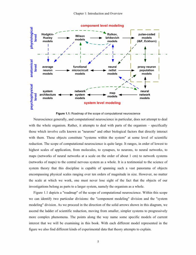
Figure 1.1: Roadmap of the scope of computational neuroscience

Neuroscience generally, and computational neuroscience in particular, does not attempt to deal

with the whole organism. Rather, it attempts to deal with parts of the organism – specifically

those which involve cells known as "neurons" and other biological factors that directly interact

with them. These objects constitute "systems within the system" at some level of scientific

reduction. The scope of computational neuroscience is quite large. It ranges, in order of lowest to

highest scales of application, from molecules, to synapses, to neurons, to neural networks, to

maps (networks of neural networks at a scale on the order of about 1 cm) to network systems

(networks of maps) to the central nervous system as a whole. It is a testimonial to the science of

system theory that this discipline is capable of spanning such a vast panorama of objects

encompassing physical scales ranging over ten orders of magnitude in size. However, no matter

the scale at which we work, one must never lose sight of the fact that the objects of our

investigations belong as parts to a larger system, namely the organism as a whole.

Figure 1.1 depicts a "roadmap" of the scope of computational neuroscience. Within this scope

we can identify two particular divisions: the "component modeling" division and the "system

modeling" division. As we proceed in the direction of the solid arrows shown in this diagram, we

ascend the ladder of scientific reduction, moving from smaller, simpler systems to progressively

more complex phenomena. The points along the way name some specific models of current

interest that we will be examining in this book. With each different model represented in the

figure we also find different kinds of experimental data that theory attempts to explain.

5


§ 2. Systems, Signals, and Information

§ 2.1. Systems and Models The science of system theory in its modern form came into being in the late 1950s, primarily

from the works of T.R. Bashkow, R.E. Bellman, and R.E. Kalman. Obviously, this science is

directed at things called "systems," but what is a system? As we might expect from a science with

the scope claimed by system theory, the definition is both broad and abstract. Webster's

Unabridged Dictionary gives us the following definition: A system is any set or arrangement of

things so related or connected as to form a unity or an organic whole.

Many people find a definition as broad and abstract as this to be unsatisfying because, as

stated in Webster's, the definition of a system would seem to suit almost anything. There is much

truth in the old saying, "That which explains everything explains nothing," and so we often find

various specialists within system theory applying more specialized definitions. Some of these

definitions are hardly any less abstract than the one just given. For example, A.D. Hall and R.E.

Fagen define a system as,

A system is a set of objects together with relationships between the objects and between their attributes [HALL].

If we take the word "object" to mean "thing" and assume that "relationships" implies these things

are related, this definition adds nothing to our previous definition except the idea that the things

making up the system have attributes, and that these attributes are also related to one another.

A great many system theorists – probably the majority – are engineers or work in an

engineering environment. Because engineers are usually concerned with being able to build

things, they prefer a tighter definition than either of those given so far. For example, Robert A.

Gabel and Richard A. Roberts defined a system this way:

A system is a mathematical model or abstraction of a physical process that relates inputs or external forces to the output or response of the system. Input and output share a cause-effect relationship [GABE: 2].

What we see added here to the definition of a system is the idea of how to describe it. We also see

something else coming into play here, namely a distinction between "the description of a physical

process" (the system) and the thing being described. Here a system is a "model" rather than the

thing being modeled. The earlier definitions were ontological (definitions of "things"); the Gabel-

Roberts definition is epistemological (definition in terms of one's knowledge of a thing).

Although this might seem like a mere difference in semantics or only a philosophical

distinction, the definition one chooses to use has an important bearing on how one thinks about a

6


scientific problem. A definition like that of Gabel and Roberts explicitly confesses that there are

things about the object being studied of which we remain ignorant, and implicitly suggests that

those things of which we are ignorant are also things with which we are unconcerned. The

obvious objection one might raise to this viewpoint is, "How do we know that the things of which

we are ignorant in our study of an object are things we can be unconcerned with?" This is the

perennial question that always comes up where mathematical science interfaces with physical

science.

Immanuel Kant, the great 18th century philosopher, recognized this issue in science more than

a century and a half before the birth of modern system theory. There is, he tells us, two sides to

the issue which, while distinct, are inseparable. These are: the epistemological side of the issue

and the practical side of the issue. Kant therefore bequeaths to us a two-pronged definition of

"system." Seen from the perspective of epistemology, a system is the unity of various knowledge

under one idea, and the object which contains this unity is called "the" system. But seen from a

practical perspective, a system is a set of interdependent relationships constituting an object

with stable properties, independently of the possible variations of its elements. If we are to call

what we do "science," we cannot separate what we know (or think we know) from the object of

our inquiry. A system, then, consists of both the object of our study and our representation

(model) of that object, and the first criterion of truth in system theory can then be seen to be the

congruence of the object with our representations of that object. This, of course, is the point

where observation and experiment enter in to science. A system theorist is not granted a license to

engage in free mathematical speculations independently of facts emerging from the laboratory.

Thus, while it is true that system theory is a largely mathematical science, it is at the same time

no less an experimental science. Its theories must have testable consequences.

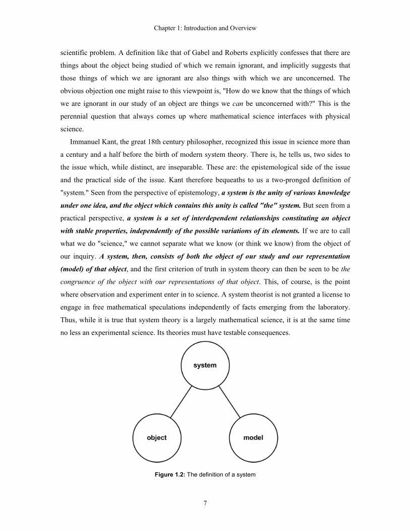
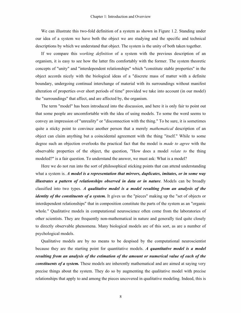
Figure 1.2: The definition of a system

7


We can illustrate this two-fold definition of a system as shown in Figure 1.2. Standing under

our idea of a system we have both the object we are studying and the specific and technical

descriptions by which we understand that object. The system is the unity of both taken together.

If we compare this working definition of a system with the previous description of an

organism, it is easy to see how the latter fits comfortably with the former. The system theoretic

concepts of "unity" and "interdependent relationships" which "constitute stable properties" in the

object accords nicely with the biological ideas of a "discrete mass of matter with a definite

boundary, undergoing continual interchange of material with its surroundings without manifest

alteration of properties over short periods of time" provided we take into account (in our model)

the "surroundings" that affect, and are affected by, the organism.

The term "model" has been introduced into the discussion, and here it is only fair to point out

that some people are uncomfortable with the idea of using models. To some the word seems to

convey an impression of "unreality" or "disconnection with the thing." To be sure, it is sometimes

quite a sticky point to convince another person that a merely mathematical description of an

object can claim anything but a coincidental agreement with the thing "itself." While to some

degree such an objection overlooks the practical fact that the model is made to agree with the

observable properties of the object, the question, "How does a model relate to the thing

modeled?" is a fair question. To understand the answer, we must ask: What is a model?

Here we do not run into the sort of philosophical sticking points that can attend understanding

what a system is. A model is a representation that mirrors, duplicates, imitates, or in some way

illustrates a pattern of relationships observed in data or in nature. Models can be broadly

classified into two types. A qualitative model is a model resulting from an analysis of the

identity of the constituents of a system. It gives us the "pieces" making up the "set of objects or

interdependent relationships" that in composition constitute the parts of the system as an "organic

whole." Qualitative models in computational neuroscience often come from the laboratories of

other scientists. They are frequently non-mathematical in nature and generally tied quite closely

to directly observable phenomena. Many biological models are of this sort, as are a number of

psychological models.

Qualitative models are by no means to be despised by the computational neuroscientist

because they are the starting point for quantitative models. A quantitative model is a model

resulting from an analysis of the estimation of the amount or numerical value of each of the

constituents of a system. These models are inherently mathematical and are aimed at saying very

precise things about the system. They do so by augmenting the qualitative model with precise

relationships that apply to and among the pieces uncovered in qualitative modeling. Indeed, this is

8


where specific relationships are introduced into a system. The vehicle by which these

relationships are introduced is called the structure of the system.

What is meant by this term? One of the best definitions given for this term was put forward by

the great twentieth century psychologist, Jean Piaget: A structure is a system of self-organizing

transformations such that: (1) no new element engendered by their operation breaks the

boundaries of the system; (2) the transformations of the system do not involve elements outside

it; and (3) the system may have sub-systems differentiated within the whole of the system and

have transformations from one sub-system to another. The obvious question raised by this

definition is: What is a "transformation"? That is what we will take up next.

§ 2.2 Signals, Information, and Transformations

To understand the quantitative concept of a transformation we must first understand what a

signal is. A signal is any physical quantity that can be represented as a single-valued function

of time and that is said to carry information. The idea of a "physical quantity" is clear enough.

By "single-valued function of time" we mean that at any particular moment in time the signal

must have a unique numerical or symbolic determination. But what does this word "information"

mean? That is a somewhat trickier question.

As it is used in the physical and mathematical sciences, the word information is employed in a

more restrictive sense than we use in everyday language. Indeed, it is used in a sense much closer

to its Latin root, informatio (a representation, an outline or sketch). The notion of information was

introduced into physics by Boltzmann in 1894, who described the thermodynamics concept of

"entropy" as a measure of "missing information." John von Neumann introduced it into quantum

mechanics and particle physics in 1932. It received a formal and rigorous treatment in the hands

of Claude Shannon in 1948 in his now classic work, "The Mathematical Theory of

Communications" (a two-part paper that appeared in The Bell System Technical Journal in 1948).

The idea was imported to biology applications by Norbert Wiener.

To appreciate how the term "information" is used here, and to clear away some of the possible

metaphysical sources of confusion that can otherwise attend its usage, let us start with the main

dictionary definitions of the verb "inform" and the noun "information."

inform, vt. [ME. informen; OFr. enformer; L. informare, to shape, fashion, represent, instruct; in, in, and formare, to form, from forma, form, shape.]

1. (a) to give form or character to; to be the formative principle of; (b) to give, imbue, or inspire with some specific quality or character; to animate.

2. to form or shape (the mind); to teach. [rare]

9


3. to give knowledge of something to; to tell; to acquaint with a fact, etc.

information, n. [OFr. information; L. informatio (-onis), a representation, an outline, sketch, from informare, to give form to, to represent, inform.]

1. an informing or being informed; especially, a telling or being told something.

2. something told; news; intelligence; word.

3. knowledge acquired in any manner; facts; data; learning; lore.

When specialized to its technical use, the word "information" takes on a connotation of how

"unexpected" or "surprising" the occurrence of a physical event is. Suppose we are measuring the

electric potential of the membrane of a neuron, and let us further suppose we observe that at any

particular moment in time this potential is either a static value of, say, -65 mV (the "resting

potential") or else it briefly pulses up to a value of, say, +20 mV (the "action potential"). The

science of information theory would then say that this neuron, viewed as an "information source,"

conveys at most 1 unit of information (the unit of measure is called a "bit"; this stands for "binary

digit") because the neuron displays only two possible activities ("rest" and "action"). More

generally, if something is capable of N distinct activities, it is said to represent at most log2(N)

"bits" of information.

An information theorist, particularly one who is interested in the theory of communication

systems, typically calls the distinct possible activities of an information source its "symbols" or

its "messages." Warren Weaver, one of the first researchers to get involved with Shannon's new

science, described "information" in the following way:

The word information, in this theory, is used in a special sense that must not be confused with its ordinary usage. In particular, information must not be confused with meaning. . . To be sure, this word information in communication theory relates not so much to what you do say, as to what you could say. That is, information is a measure of one's freedom of choice when one selects a message. If one is confronted with a very elementary situation where he has to choose one of two alternative messages, then it is arbitrarily said that the information, associated with this situation, is unity. Note that it is misleading (although often very convenient) to say that one or the other message conveys unit information. The concept of information applies not to the individual messages (as the concept of meaning would), but rather to the situation as a whole, the unit information indicating that in this situation one has an amount of freedom of choice, in selecting a message, which it is convenient to regard as a standard or unit amount [SHAN: 8-9].

The information said to be "carried" by a signal is thus a measure of the number of observable

unique ways in which that signal can behave over time. This is what is meant when one speaks of

the "degrees of freedom" an observed signal activity exhibits. (We would not say that a neuron

"chooses" what signal it is going to exhibit at any particular moment in time, and so "degrees of

freedom" is a more appropriate description than "freedom of choice"). The principal challenge in

10


applying information theory to biological signal processing lies in determining what constitutes

the "message" or "symbol" said to be represented by the signal. This is because information

theory is utterly silent on the topic of the "meaning" of a signal.

Any physical quantity said to constitute a "signal" always, by implied definition, is one that

conveys or produces a physical relationship between two or more of the objects that make up the

system. Specifically, this relationship is one of causality and dependency. The object that

generates (produces) the signal is called the source of the signal, and the object or objects upon

which this signal acts to produce some kind of physical change is called the destination of the

signal. The source is said to be a "cause" of activity (in the case where there are multiple sources

sending signals that converge on a common destination, a particular source is called a "partial

cause"). The way in which a signal affects the destination object is called its "effect." We may

note that this way of using the otherwise metaphysical terms cause and effect constitutes a

practical "working definition" of these terms in biological signal processing. (As Kant put it, this

kind of definition is one "which makes a concept useful in practice").

Now because a signal produces a change of some kind in the destination object, the way this

object responds to that signal, or to other subsequent signals it "receives," is called a

transformation, and the signal is said to effect a transformation in the behavior of the system.

When the signals involved are internal to the system (that is, the signals are regarded as neither

impinging upon the system from without nor merely leaving the system to serve as 'inputs' to

another system), the transformation effected is called a self-regulating transformation (because

we are dealing with a situation where the system is said to 'act upon itself'). Because there can be

many ways in which a system can 'act upon itself,' there can be many different transformations

possible within the system. The formal mathematical description of all these transformations,

subject to the other two constraints given earlier, is the mathematical structure of the system.

§ 2.3 System Modeling

Making the model of a system is called modeling the system. It is a necessary first step in

obtaining a quantitative description of the object being studied. Development or identification of

the mathematical structure of the system is always done first. The usual procedure is to begin

with the qualitative model deduced from experiments (either biological or psychological), and

then re-cast this model in a mathematical description. This will typically result in some set of

mathematical equations relating the various objects within the system.

In addition to the logical and mathematical relations and functions contained in this

description, the model equations will also contain two other distinguishable constituents:

11


variables and parameters. A mathematical variable represents something that can change in time

and which often represents a signal. A parameter is some quantity that describes the system but

which is typically not regarded as being representative of the activity of the system. Rather, it is

regarded as a quantity which determines how system activity is related to the signal variables. For

example, in Newton's famous F = m⋅a equation, F (force) and a (acceleration) are variables

whereas m (mass) is a parameter.

This seemingly simple description is often made more complicated by the fact that in many

systems (including the ones we deal with in this book), the parameters are not necessarily time-

invariant. For example, a rocket in flight uses up its rocket fuel as its engines burn, and the

consumption of this fuel causes the rocket's mass to be a function of time. Nonetheless, the mass

is regarded as a parameter of the rocket-system rather than a signal variable. In modeling a

system, what is to be regarded as a "variable" and what is to be regarded as a "parameter"

depends on the purpose for which the modeler has constructed his model. If I want to fly a rocket

to the moon, force and acceleration are signals (to me) and mass is a parameter. But if I want to

match up pairs of wrestlers for a tournament, the mass of each wrestler is a "variable" I use to

determine how the wrestling meet will be "structured." We can see that the structure of a model

depends on the reason for making the model, and this is where modeling embeds some of the

character of an art in with the science that goes into making a model. It is also the reason why

there is no one unique prescription for how to build a model.

In many scientific problems, one takes advantage of a body of known facts to guess what the

structure of an accurate model might look like. There are two ways to proceed with this guessing

(which scientists call "making an hypothesis"). One is to pre-select one particular model structure

that one has reason to think is probably "an accurate description" for the system being modeled.

This is perhaps the most common approach used in the sciences, and it is based in one part on the

qualitative model from which one begins, and in another part on what one knows generally of the

anatomical, physiological, or psychological principles (in the case of computation neuroscience)

thought to govern this particular class of systems in general. This approach works best when the

scientist making the model has a good deal of experience with, and well-founded training in, the

topic at hand. It works less well when one is inexperienced or lacks adequate background training

and/or knowledge of the literature in the field. Also worthy of note, because it is something not

infrequently overlooked, is that the modeler's decisions of what to leave out of a model are

sometimes just as important as the decisions about what to put in. It is impractical to "put

everything in" and absurd to "leave everything out"; good model-makers learn how to strike the

appropriate balance between these extremes.

12


Sometimes, though, not enough is known about the object under study to come up with just

one specific model structure for turning a qualitative model into a quantitative one. Rather, one

might come up with a whole class of possible structures, each of which cannot be ruled out a

priori through one's knowledge of the object. In this case, it is usually possible to use additional

experimental outcomes to narrow down the possible structures. In system theory this is called the

structure identification problem, and system theorists have developed a number of specialized

techniques for accomplishing this. Indeed, there is within system theory an entire sub-discipline

of specialists devoted to finding better practical techniques to carry out structure identification.

One could say these people are "the model-maker's model makers."

Once a structure has been identified – by whatever means – the next step in model-making is

the estimation of the parameters of the model. Naturally, this is called the parameter estimation

problem, and a number of practical techniques for efficiently accomplishing this task from

experimental data have also been developed. Not infrequently, scientists who specialize in

structure identification are also experts in parameter estimation since the two tasks are, in a

practical sense, joined at the hip.

Some models – particularly ones for relatively simple systems – can be deduced from first

principles. Such models are widespread, for instance, in engineering. But more often – and in the

case of biological signal processing and computational neuroscience this is always the case at our

present level of knowledge – it is not possible to deduce the correct model starting with

fundamental laws of physics. The systems are simply too complicated to permit this. In these

cases, the models employed are typically either based on arguments for plausible forms of

mathematical expression – based on physical arguments, not deductions – or on arbitrary

equations with parameters chosen so that the equations "fit the data." Models of this second class

are called statistical models. They are "curve fits." Such models aid in the analysis of a system

but do not contribute to making theoretical predictions about the system.

Models of the first class, although they usually also involve some curve-fitting, are expected

to have something statistical models usually do not, namely predictive power. They achieve this

predictive power (when they achieve it) because of the physical arguments that go into

postulating the mathematical form of the structure. These models are called phenomenological

models. A phenomenological model with an established track record of making good predictions

is called a theory. One of the most important theories in neuroscience, the justly famous

Hodgkin-Huxley model, is none other than a phenomenological model. Its discoverers, Alan

Hodgkin and Andrew Huxley, won the 1963 Nobel Prize in medicine for this model.

13


§ 3. Neurons and Glial Cells

From the viewpoint of the computational neuroscientist or the biological signal processing

theorist, the central nervous system is composed of two types of cells, called neurons and glial

cells. There is, of course, more to the brain than this – e.g. blood vessels and fluid-filled cavities –

but the arena of interest for these scientists is focused on neurons and glia. It is not an equal

partnership; neurons receive far more attention than glial cells in research by computational

neuroscientists. The reason for this is mainly traditional. Neurons have long been supposed to be

the "instruments" for signal processing in the brain and spinal cord, whereas glial cells were

supposed to provide merely mechanical support and nutrition for the neurons, and to provide

"electrical insulation" for the "wiring" that interconnects neurons.

One interesting fact about the brain is that neurons have no direct input connection from the

blood vessels. This is known as the "blood-brain barrier." Glia, on the other hand, do have a

direct connection from the blood vessels. Since oxygen and nutrients are blood-borne, and since

neurons do require both an oxygen supply and a supply a nutrients to support their metabolism, it

is fair and rather safe to conclude that glia do indeed carry out this "support function." The term

"glia" is derived from a Greek word that means "glue," and for a long time no one doubted that

glia were merely the glue that held the brain together.

Today we are not so sure. It has long been known that glia regulate the levels of various ions

in the fluid-filled spaces surrounding neurons, and it has likewise been known for a long time that

the electrical properties of neuronal behavior are determined in part by this "ion bath." Still, that

regulative function carried out by glial cells can be regarded, using electrical engineering

terminology, as a "bias function." This would make the vast network of glial cells a kind of

biological "biasing circuit." Since "bias" is not usually regarded as being part of signal processing

(the "bias variable" is said to carry no "information"), there was and is no reason, strictly on this

account, to regard glia as part of the signal processing system.

However, there have been experimental findings reported over the past decade that indicate

glial cells might have a signal processing role after all. Much of this is very speculative at this

time. However, there are some facts about glial cell activity that are very well established. One of

the most important of these (in the opinion of your author) is the finding that glial cells transfer

calcium ions (Ca2+) to various locations in the brain, and seem to do so in response to signaling

activities. Ca2+ is a very, very important chemical involved in the signal processing functions of

neurons, and the fact that glial cells transport it around implicates for them some important role in

the large scale behavior of neural network activity. Unfortunately, it is still far from clear just

14


what, precisely, the role of this "calcium signaling" might be. Still, it is not too bold to speculate

that the coming years will bring major changes in the way we look at and model biological signal

processing in the central nervous system (CNS).

The signal processing role of neurons is definitely far better established. The membrane of a

neuron cell is excitable – a term that means an electric potential is developed across it, and this

potential responds dramatically to input signals the neuron receives from other neurons. A typical

membrane potential, referenced to the fluid surrounding the neuron, is on the order of about –65

mV in experiments done in vitro. There is a great deal of variance in this value for different kinds

of neuron cells in vivo and in different regions of the CNS. The value of this potential difference

between the inside ("cytoplasm") and the outside ("extracellular region") of the neuron, in the

absence of activity at the neuron's inputs and outputs, is called the resting potential of the cell.

Most (but not all) neurons can be stimulated by their inputs into producing a large change in the

membrane potential – typically the potential shoots up to on the order of about +20 mV – for a

brief period of time (on the order of about 1 ms). This is called the action potential. Other

neurons, which do not produce an action potential "spike" in response to stimuli, nonetheless do

show a lesser but still significant (tens of mV) change in their membrane potential; in their case

this is called a graded response.1

Biologists estimate there is on the order of about ten thousand different species of neurons,

and within each species there are many variations. Nonetheless, from a functional point of view

most neurons can be represented in terms of a single general model composed of four basic signal

processing components. This is illustrated in Figure 1.3. The four components of the model

neuron are: (1) the input component; (2) the integrative component; (3) the conductile

component; and (4) the output component.

Figure 1.3: Model Neuron

1 It is worth noting that glial cells also have a non-zero membrane potential and also exhibit a graded response when their nearby neurons are active. However, the magnitude of this response is much, much less than that of a neuron (typically only a few millivolts). For this reason, glia are said to not be excitable. It is a relative terminology.

15


The input component is the part of the neuron that receives signals from other neurons. The

actual point of signal connection between the source neuron and the destination neuron is called a

synapse (the word is derived from a Greek word that means "to connect").2 Typically a synapse is

characterized by at least two parts, a part that is physically part of the source neuron (called the

"presynaptic component" of the synapse) and a part that is physically part of the destination

neuron (called the "postsynaptic component" of the synapse). Thus, a synapse is a biological

structure that "belongs" communally to both neurons. In biological terminology, the source

neuron is called the presynaptic cell, and the destination neuron is called the postsynaptic cell.

On the average, a typical neuron may have on the order of about 20,000 synapses (in the monkey

neocortex), although some neurons have far fewer than this and some have far more. (The

Purkinje cell in the human cerebellum is thought to have on the order of about 200,000 synaptic

inputs, and a typical motor neuron in the spinal cord has on the order of about 50,000 synaptic

inputs).

The integrative component, as the name implies, sums the postsynaptic signals resulting from

synaptic activity. Biologically, the quantities being summed are typically ion currents that were

produced by the postsynaptic cell's response to synaptic inputs. Positive ions flowing into the cell

(such as Na+ or Ca2+) and negative ions flowing out of the cell (such as Cl -) are said to be

excitatory because these currents tend to stimulate the neuron into producing and transmitting its

own signal to the output component. Positive ions flowing out of the cell (such as K+) are said to

be inhibitory because these currents tend to prevent the neuron from generating its own output

signal. Different types of synapses are characterized by the types of ion currents they produce,

and are thus called excitatory or inhibitory synapses. The integrative component also contains a

variety of membrane-spanning proteins (called voltage-gated channels) that open or close in

response to the electric potential induced by the ions currents entering and leaving the integrative

region of the neuron. When open, these proteins conduct additional ion currents into or out of the

cell. Thus, they act like a kind of electrically-stimulated valve. The region of highest

concentration of these voltage-gated channels (VGCs) is called the trigger zone because it is in

this region that the neuron's output response to its synaptic inputs is generated. In neurons that

generate an action potential response (called spiking neurons), the trigger zone is often an easily-

2 We are speaking here of the usual case. There is evidence that some neuron-to-neuron signaling takes place when one neuron produces and emits small molecules, such as nitrous oxide (NO), that easily pass through the cell membranes. In this case, there is no observable direct connection between the neurons and no synapse transmitting the signal. This is called "non-synaptic transmission" and we can think of it as the neuronal equivalent of "broadcasting." In neuroscience there is almost no statement we can make that is always true without exception, and this is something the non-biologist must get used to when reading the literature on neuroscience.

16


identifiable region of the cell. In neurons that produce a graded response (which we will call

graded neurons), the VGCs tend to be more widely distributed and the trigger zone is more

difficult to define. Some scientists would say that a graded neuron has no trigger zone, preferring

to reserve this term for spiking neurons only.

The conductile region, as the name suggests, conducts the neuron's response signal from the

integrative component to the neuron's output component. In many neurons, the conductile

component is an easily-identifiable part of the neuron called an axon. In neurons that have an

axon, the method of signal transmission is often very interesting. Rather than acting merely like a

cable that passively conducts current and voltage from one place to another, the axon acts more

like a repeater network. VGCs are spaced at intervals along the axon and regenerate the action

potential. (This is called saltatory conduction; the word saltatory comes from the Latin word

saltus, which means "jump" or "leap"). This is the primary means by which signals are

transmitted over long distances in the CNS. For example, some neurons in the motor cortex

region of the brain (located in the brain region nearest the top of the head in humans) project

axons that run to the bottom segments of the spinal cord. Some motor neurons in the spinal cord

project to the muscle tissue in the toes. Some axons are on the order of 1.5 meters in length, and

signal transmission in these cases would not be possible without this "repeater action" of the

conductile component.3

The output component is the part of the neuron that connects to other neurons (or, in the case

of motor neurons, to the muscle tissue these neurons stimulate). Graded neurons typically connect

to other neurons via a class of synapse called a gap junction. A gap junction synapse basically

acts like a valve that opens and allows direct ionic current flow to take place between neurons. In

most cases this current can flow in either direction and the gap junction can be modeled as a

simple electric resistor. Networks of neurons interconnected by these gap junctions effectively act

like one gigantic neuron. This kind of network is sometimes called a syncytium, although many

biologists dislike applying this term to neural networks.4 Networks of glial cells are also

interconnected by means of gap junctions. In some cases, a gap junction might conduct ion

current in only one direction. These are called rectifying gap junctions, and they are modeled as a

resistor in series with a diode.

In mammals, by far the most common type of output component converts the incoming

electrical signal to a chemical signal. This type of synapse is called a chemical synapse. The

3 Neurodegenerative diseases such as multiple sclerosis kill the glial cells that insulate the axon. This eventually results in failure of the saltatory conduction mechanism. 4 This dislike stems from a great controversy that took place at the end of the nineteenth and beginning of the twentieth century between what was known as the reticular theory and the cell theory.

17


arrival of an action potential at the presynaptic terminal of the source neuron stimulates the

secretion of chemicals into a tiny gap (called the synaptic cleft) that separates the presynaptic and

postsynaptic neurons. This process is called neurotransmitter exocytosis. These small molecule

neurotransmitters bind to receptor proteins in the postsynaptic cell, and thereby trigger a response

in that cell. This response is called the postsynaptic response. The action of a chemical synapse is

sometimes puckishly described as "communicating by smoke signals," which is, interestingly

enough, not too bad a metaphor.5

Despite the great variety in neuron types, most neurons can be placed in one of two general

classes. The first class is called the projection neuron class. Projection neurons are also

sometimes called principal neurons or relay neurons. The second class is called the interneuron

class (also called the intrinsic neuron class). Projection neurons are characterized by possession

of a well-defined single long axon that makes distant connections. The axon will also usually give

off branches, as suggested by the output section depicted in Figure 1.3. Large axons and their

branches are often (but not always) wrapped in a myelin sheath of covering glial cells, which

insulate the axon and improve signal propagation along it.

Interneurons have either a very short axon or no axon at all. In the latter case the neuron is

called an "anaxonal" or an "amacrine" (a, no, and macrine, long projection) or a "granule" cell.

Like the projection neuron, most interneurons do express other projections away from the cell

body. These projections are called dendrites. In a projection neuron dendrites are part of the

anatomical structure of the cell that serve the input function. In interneurons dendrites serve both

the input and the output functions. All neurons have a cell body, called the soma, that contains the

cell's nucleus. Thus, the soma, dendrites, and axon (when it has one) make up the anatomy of the

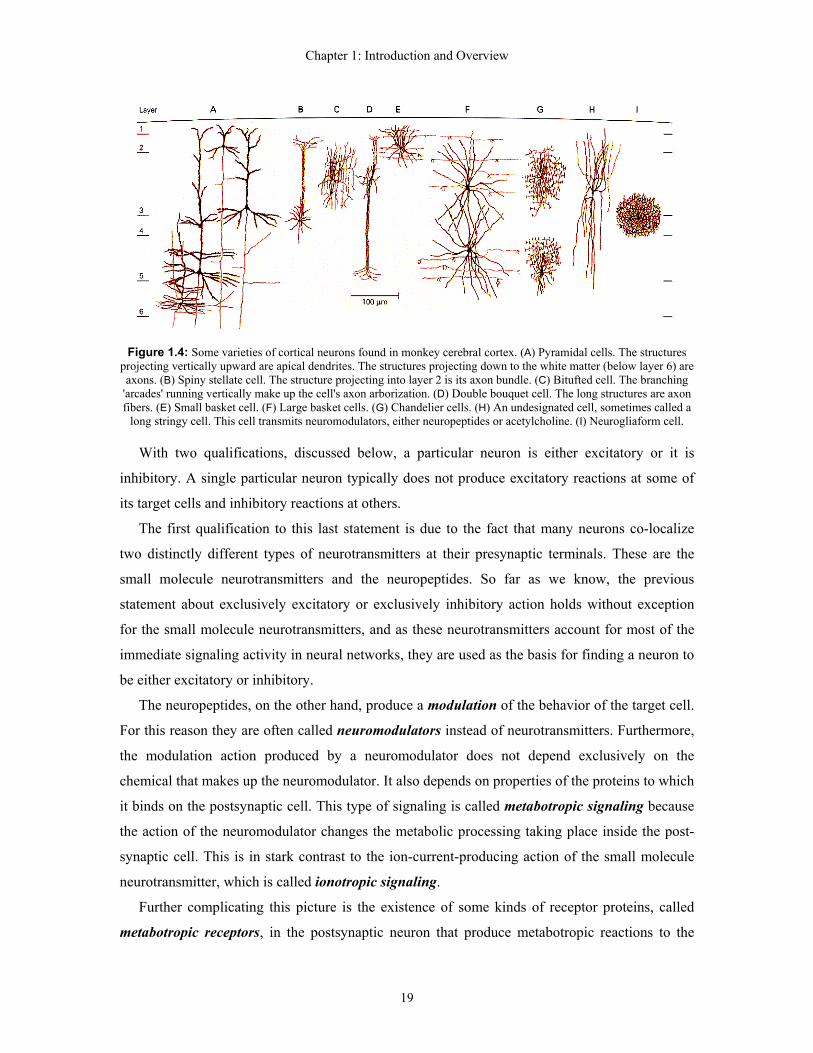
neuron. Some appreciation for the great variety of neurons can be gained from Figure 1.4, which

illustrates some of the various types of neurons found in the cerebral cortex of the monkey.

Neurons are also broadly classified as either excitatory or inhibitory cells. Excitatory cells

produce output signals that tend to either evoke or promote the generation of an output response

(typically an action potential) from their target destination cells. For the cells illustrated in Figure

1.4, the pyramidal cells (A) and the spiny stellate cell (B) are excitatory cells. All the others are

inhibitory cells. Inhibitory cells produce output signals that tend to inhibit the destination cells

from producing an output response.

5 This clean dichotomy is marred somewhat by the fact that some neurons do not fit into either class. In particular, some neurons express both gap junction and chemical synapses, and exhibit a small spiking response within a graded response. Neurons of this sort exist, for example, in the retina of the eye. As noted earlier, there are very few things we can say in general that do not have exceptions to the rule in neuro-science.

18


Figure 1.4: Some varieties of cortical neurons found in monkey cerebral cortex. (A) Pyramidal cells. The structures

projecting vertically upward are apical dendrites. The structures projecting down to the white matter (below layer 6) are axons. (B) Spiny stellate cell. The structure projecting into layer 2 is its axon bundle. (C) Bitufted cell. The branching

'arcades' running vertically make up the cell's axon arborization. (D) Double bouquet cell. The long structures are axon fibers. (E) Small basket cell. (F) Large basket cells. (G) Chandelier cells. (H) An undesignated cell, sometimes called a

long stringy cell. This cell transmits neuromodulators, either neuropeptides or acetylcholine. (I) Neurogliaform cell.

With two qualifications, discussed below, a particular neuron is either excitatory or it is

inhibitory. A single particular neuron typically does not produce excitatory reactions at some of

its target cells and inhibitory reactions at others.

The first qualification to this last statement is due to the fact that many neurons co-localize

two distinctly different types of neurotransmitters at their presynaptic terminals. These are the

small molecule neurotransmitters and the neuropeptides. So far as we know, the previous

statement about exclusively excitatory or exclusively inhibitory action holds without exception

for the small molecule neurotransmitters, and as these neurotransmitters account for most of the

immediate signaling activity in neural networks, they are used as the basis for finding a neuron to

be either excitatory or inhibitory.

The neuropeptides, on the other hand, produce a modulation of the behavior of the target cell.

For this reason they are often called neuromodulators instead of neurotransmitters. Furthermore,

the modulation action produced by a neuromodulator does not depend exclusively on the

chemical that makes up the neuromodulator. It also depends on properties of the proteins to which

it binds on the postsynaptic cell. This type of signaling is called metabotropic signaling because

the action of the neuromodulator changes the metabolic processing taking place inside the post-

synaptic cell. This is in stark contrast to the ion-current-producing action of the small molecule

neurotransmitter, which is called ionotropic signaling.

Further complicating this picture is the existence of some kinds of receptor proteins, called

metabotropic receptors, in the postsynaptic neuron that produce metabotropic reactions to the

19


small molecule neurotransmitters. These receptors are quite distinct from the ones that produce an

ionotropic reaction in the postsynaptic cell (which are called ionotropic receptors). The synapse

can contain both kinds of proteins at the same site. Finally, there are some kinds of small

molecule neurotransmitters (specifically, dopamine, serotonin, and norepinephrine6) that produce

metabotropic reactions in the target cell. These kinds of synapses constitute the second

qualification of our earlier statement. We presently know of no major ionotropic receptors for

dopamine or norepinephrine in the brain and only one ionotropic receptor (5HT3) for serotonin.

Ionotropic signaling is fast. Reactions to ionotropic signals take place on the order of about a 1

ms time scale. They are also short duration events, their effects disappearing within a few

milliseconds. Because of this, it is a reasonable hypothesis that ionotropic signals represent, to

use the language of signal processing theory, "real-time data processing." Metabotropic signaling,

on the other hand, is slower in onset and its effects last far longer. Metabotropic signals first

begin to show their effects tens of milliseconds to hundreds of milliseconds after the metabotropic

signal has been transmitted. Metabotropic effects can last from many tens of milliseconds, to

hundreds of milliseconds, to seconds, to minutes, to hours. Some metabotropic effects are so long

lasting as to be effectively permanent. These latter effects are thought to be the biological basis

for long-term memory and learning.

Thus, biological signal processing involves two distinct types of signaling activities. We

may call these "data processing activities" (ionotropic signaling) and "modulation, control, and

adaptation activities" (metabotropic signaling). The classifications are hypothetical at our present

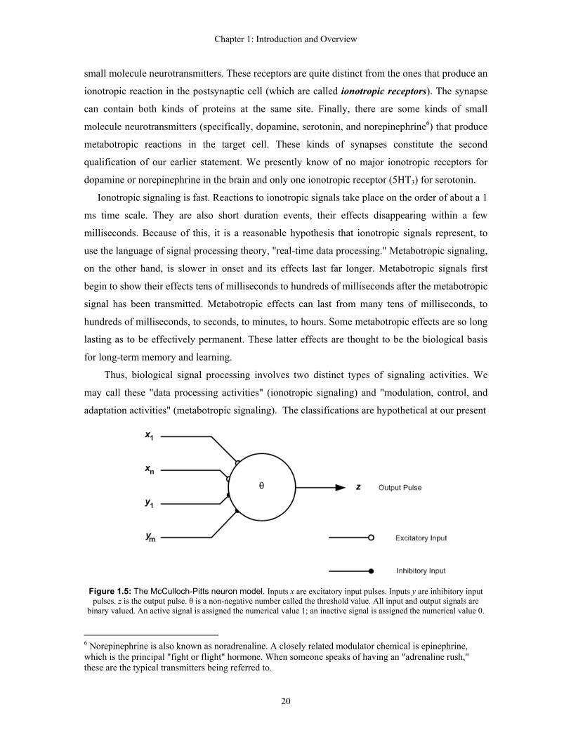
Figure 1.5: The McCulloch-Pitts neuron model. Inputs x are excitatory input pulses. Inputs y are inhibitory input pulses. z is the output pulse. θ is a non-negative number called the threshold value. All input and output signals are

binary valued. An active signal is assigned the numerical value 1; an inactive signal is assigned the numerical value 0.

6 Norepinephrine is also known as noradrenaline. A closely related modulator chemical is epinephrine, which is the principal "fight or flight" hormone. When someone speaks of having an "adrenaline rush," these are the typical transmitters being referred to.

20


state of knowledge. Nonetheless, this hypothesis seems to be a reasonable description of the

probable role of these two very different signal processes. Of these two signal processes, the

ionotropic signaling process is unquestionably the one that has received the most study. Our

knowledge of metabotropic signal processing is significantly less advanced at present.

§ 4. Early Neural Network Theory

The existence of spiking neurons was known well before Hodgkin and Huxley carried out

their epic research that led to the theory of the detailed physiology of neural signaling. In 1943

neurologist Warren S. McCulloch and his associate Walter Pitts published the first mathematical

model of the neuron and laid the foundations for the theory of neural networks [McCU]. Their

subsequent work [PITT] introduced theoretical issues that are still key research topics in neural

network theory today.

Figure 1.5 illustrates the original McCulloch-Pitts neuron model. Input signal vectors x and y,

and output signal z, are binary-valued pulses taking on values of either 0 (inactive) or 1 (active). θ

is a non-negative number called the threshold. The value of the output pulse z is determined by

the relationship between the excitatory inputs (x) and the inhibitory inputs (y) defined by

. (1.1)

>−

≤−

=

∑∑

∑∑

==

==

θif1

θif0

11

11m

jj

n

ii

m

jj

n

ii

yx

yxz

This simple model captured what was known of neurodynamics at that time. Such a simple

model probably would not have attracted much attention except for McCulloch's and Pitts' major

finding. They were able to prove that any finite logical proposition can be expressed by a network

of McCulloch-Pitts neurons. This result caused a great stir because in 1943 many people were

followers of a pseudo-philosophical attitude known as logical positivism. Among other things,

logical positivism speculated that formal logic constituted the basic rules by which thinking takes

place. This happy hypothesis has since been refuted by psychological research, but it was very

influential throughout the 1940s and 50s. If neural networks could implement any logic function,

the thinking went, then the McCulloch-Pitts theory drew the shades back from the great mystery

of how thinking works in the brain. In the long run, the McCulloch-Pitts model proved to be more

influential with computer scientists than with neurophysiologists, but it was nonetheless a seminal

work. The McCulloch-Pitts model still pops up from time to time in network research.

The work of McCulloch and Pitts soon came to the attention of one of the more remarkable

21


figures in twentieth century mathematics, John von Neumann. Von Neumann was able to prove

that any McCulloch-Pitts neuron could be built up from a small set of simpler McCulloch-Pitts

neurons, which von Neumann termed "organs" [NEUM1]. He used this fact in his pioneering

work that led to the development of the digital computer. Von Neumann's "organs" are today

known as "logic gates," and the central processing unit of the modern computer is nothing else

than an artificial neural network constructed from McCulloch-Pitts neurons. This, by the way, had

a lot to do with why early computers were popularly called "electronic brains" throughout the

1950s and on into the early 1960s. Indeed, von Neumann's speculations on the relationship

between computers and brains contain a number of remarkably prescient insights still important

today [NEUM2-3].

Von Neumann's early death from cancer left the task of developing the mathematical theory of

neural networks in the hands of other, mostly younger, pioneers. Two most notable early

explorers were psychologist Frank Rosenblatt and a young electrical engineer named Bernard

Widrow. Working independently, Rosenblatt and Widrow introduced, at almost the same time,

two significant and very similar extensions of the McCulloch-Pitts-von Neumann model.

Rosenblatt called his model the perceptron [ROSE1-3]; Widrow called his the Adaline [WIDR1-

3].

The perceptron and the Adaline both extended the capabilities of the McCulloch-Pitts model,

but, more importantly, both models introduced adaptation algorithms by which they could be

trained by examples to implement desired logic and signal processing functions. Rosenblatt called

his algorithm the perceptron rule. Widrow's algorithm was originally known as the Widrow-Hoff

or delta rule, but has since become more widely known as the LMS algorithm.7 Although both

models and even both algorithms are very similar – so similar that many young researchers today

mistakenly think the perceptron and the Adaline are one and the same8 – there are some very

important differences in how the two models perform [WIDR3]. Early perceptron researchers

made a number of speculations on what the perceptron was potentially capable of doing that

turned out to be untrue. These claims were brilliantly, and somewhat harshly, refuted in a 1968

book by Marvin Minsky (one of the early pioneers of artificial intelligence) and Seymour Papert

[MINS]. Minsky and Papert proved a number of theorems showing that what a perceptron could

really accomplish was, in fact, rather limited. Their work brought to an end the line of

investigation that originated from the original perceptron concept.

7 LMS stands for "least mean squared." 8 Only the adaptive threshold part of a perceptron is like an Adaline, but even here the differences are important.

22


The Adaline and the LMS algorithm proved to be more hardy. Although some of Minsky's and

Papert's theorems apply equally to the original Adaline, it turned out that networks of Adalines

(called Madaline networks; Madaline stands for "many Adalines") overcome a number of the

limitations of perceptron networks, and later enhancements to the original Adaline overcame even

more. Thus, the Adaline and Madaline networks are still alive and well today, particularly in the

field of neural network modeling of psychological phenomena.9 Furthermore, the linear core of

the Adaline (called the adaptive linear combiner) proved to have a multitude of important

applications in adaptive filtering and adaptive signal processing extending far outside the realm of

neural network theory. Today the LMS algorithm is probably the most widely used algorithm

across the entire field of adaptive signal processing and adaptive image processing.10

Minsky's and Papert's book also had an important unintended consequence. Their masterful,

rigorous, and authoritative treatment of the perceptron's limitations convinced program officers at

U.S. federal funding agencies that further funding of neural network research was throwing

money down a rat hole. The funding stopped and the decade of the 1970s became a kind of dark

age for neural network theory. Naturally, Minsky and Papert got blamed for this, and even today,

long after the rebirth of widespread neural network research in the 1980s, some older researchers

still bristle and snarl at the mere mention of Minsky and Papert.

Yet although there was this mass extinction event for active neural network researchers, the

species did not altogether die out in the 1970s. In Germany (where he was beyond the reach of

U.S. funding agencies), Christoph von der Malsburg [MALS1] was carrying out research that led

in time to the correlation theory of brain function, which is today one of the most important

fields of study in computational neuroscience [MALS2]. Paul Werbos discovered the

backpropagation algorithm [WERB]. As is not unusual for a dark age, Werbos' algorithm

remained in obscurity until it was re-discovered by Rumelhart et al. in 1985 [RUME1]. This re-

discovery brought the 1960s perceptron and Madaline networks line of research back from the

grave and re-populated the species of neural network theorists. The new twist in the neuron

models used in backpropagation schemes (and other schemes developed since then) is the

replacement of the binary-valued output of the perceptron and original Adaline models by a

9 Your author feels obligated to say that some of the more important issues raised by Minsky and Papert are probably (in his opinion) still issues even for today's modern versions of Madaline and other connectionist networks. The new Adaline derivatives are different enough that the conditions for the Minsky-Papert theorems no longer apply; but this only means there are no theorems telling us whether or not the old problems are still with us. It is a neglected area of mathematical neural network research. 10 Here it must be noted that there are actually two versions of the LMS algorithm. They are called the α-LMS and the µ-LMS algorithms [WIDR3]. It is the µ-LMS algorithm that finds the widest usage outside the field of neural network theory.

23


continuous-valued output function (now called the activation function). These extended models

are sometimes called generic connectionist models, and are sometimes called firing rate models.

But probably the most significant figure of this era was Stephen Grossberg. From his earliest

work in the 1960s and up to the present day, Grossberg is the father of a completely distinct

branch of neural network theory that has always been firmly rooted in neuroscience and remains

faithful to that research mission today [GROS1-10], [ELIA]. By the mid-1970s Grossberg's work

had led to the development of adaptive resonance theory (ART) [CARP1-5], [GROS5-6]. Every

passing year seems to bring more evidence to light that ART touches something fundamental

about brain function. He has from time to time been harsh and blunt in his criticisms of other

neural network modelers and theorists for engaging in romantic speculations not anchored in

psychophysical facts. This has not made him very popular, but his work is nonetheless widely

recognized as among the most important in computational neuroscience.

§ 5. Pulse-mode Neural Network Models

One feature common to all the post-McCulloch-Pitts models just discussed is their distance

from the individual biological neuron. Although the basic units employed in all these networks

are called "neurons" in the literature, the fact is that few biologists would recognize them as such

were they not told that these mathematical entities are "neurons." What these models do is

attempt to model the large-scale behavior of groups of many neurons. They are populations-of-

neurons models rather than neuron models. There is a great deal of pragmatism in this approach

because even very small patches of brain tissue involve hundreds to thousands of closely-

interconnected biological neurons. Current estimates place the total number of neurons in the

human brain as being on the order of 100 billion neurons with on the order of 100 trillion

synapses. Even relatively small areas of the brain that can be correlated to psychological

phenomena quickly run to hundreds of thousands or even millions of neurons. The computational

issues that attend modeling such vast numbers of neurons are staggering, and the problem of

interpreting what such models are doing is even more staggering. Sejnowski et al. comment,

One modeling strategy consists of a very large scale simulation that tries to incorporate as much of the cellular detail as is available. We call these realistic brain models. While this approach to simulation can be very useful, the realism of the model is both a weakness and a strength. As the model is made increasingly realistic by adding more variables and more parameters, the danger is that the simulation ends up as poorly understood as the nervous system itself. Equally worrisome, since we do not yet know all the cellular details, is that there may be important features that are being inadvertently left out, thus invalidating the results. Finally, realistic simulations are highly computation-intensive. Present constraints limit simulations to tiny nervous systems or small components of more complex systems. Only recently has sufficient computing power been available to go beyond the simplest models [SEJN1].

24


Much of the challenge in computational neuroscience is attending to the dual problems of

managing scale and connecting different levels of scale in an orderly hierarchy of scientific

reduction (figure 1.1). Models such as those discussed in §4 are aimed at understanding larger-

scale psychophysical phenomena. Coming up from the lower level of neuron-scale physiological

phenomena are the pulse-mode neuron and pulse-mode neural network models.

Unlike the case of the higher-level models of §4, a well-trained anatomist or physiologist can

look at these models and their outcomes and be able to quickly judge whether or not to believe

the model and to see how one could go about verifying the predictions of these models in the

laboratory. When the day arrives where we can trace an unbroken path from physiological neuron

models all the way up to the systematic models of the type described in figure 1.1, we will know

that neuroscience has matured to a degree matching the maturity of physics. Until that day, the

systematic populations-of-neurons models will labor under a well-justified suspicion that they

might be nothing more than Platonic exercises in mathematics. This is something every

computational neuroscientist needs to clearly understand. Our goal is to make biological theory

and psychophysical theory "meet in the middle."

A strong case can be argued for assigning the birthday of computational neuroscience to the

appearance in 1952 of Hodgkin's and Huxley's landmark paper [HODG], the work for which they

won the Nobel Prize. At that time the term "computational neuroscience" was still years away

from being introduced. Indeed, even "neuroscience" as an identifiable discipline was still years

away from being recognized. The Hodgkin-Huxley model was, and still is, regarded first and

foremost as a work of physiology. Computers were an expensive rarity at that time11, and there

was no question of, or probably even the thought of, running simulations based on the Hodgkin-

Huxley model. It would not be until the 1970s that we would see an explosive growth in the

development and use of Hodgkin-Huxley derivative models for providing theoretical explanations

of physiological findings of neuron behavior and for simulating small neural netlets of what

Sejnowski et al. called the "realistic models" class in the quote above.

Although the H-H model was phenomenological, the physical reasoning upon which it was

built gave a direction to research at the sub-neuron level. The much more recent confirmation at

the protein level of what must have been seen in 1952 as a highly speculative hypothesis, is a

stunning testimonial to Hodgkin's and Huxley's insight. Today Hodgkin-Huxley models set the

standard against which the accuracy of newer and less computationally-expensive pulse-mode

neuron models are judged.

Pulse-mode neuron modeling research has branched out from the H-H model in two different 11 International Business Machines (IBM) was still a year away from announcing its first computer.

25


directions. We can more or less accurately call these two branches the physiological branch and

the signaling branch. The physiological branch remains very closely tied to the physiologist's

laboratory, and it focuses on providing quantitative explanations for laboratory results. The 1952

Hodgkin-Huxley model was a quantitative model of the giant axon of the squid, not a "model of

everything." The enduring contribution of the H-H model is in (1) the physiological insight it

provided, and (2) its power and generality as a modeling method. (The latter is what is meant by

calling later models H-H derivatives). Work in the physiological branch faces in one of two

directions: either inside the neuron, to explain at a more primitive level the neuron's behavior, or

outside the neuron, to understand the physiological properties and behaviors of small assemblies

of neurons. Examples of the first kind are provided by the work of J.A. Connor [CONN1-2] and

the outstanding team of D.A. McCormick and J.R. Huguenard [McCO], [HUGU]. An excellent

representative of the second kind is provided by the work of H.R. Wilson [WILS1].

Neuron models tied closely to physiological mechanisms are computationally expensive and

this limits their applicability to only very small networks. The signaling branch of research

attempts to understand the signal processing going on in biological neural networks. Here greatly

simplified neuron models are employed, sacrificing physiological fidelity in favor of fidelity in

signaling properties within much larger neural network models, in order to make orders-of-

magnitude reductions in the computational costs of these models. Indeed, it is often misleading to

call the "neuron" models used in these networks "neurons" because what they often represent are

the cooperative behaviors of groups of neurons (but at a level of scale far lower than that of the

models of §4). The most widely used "neuron" models of this branch all belong to this class of

abstract cell-group models.

The simplest pulse-mode neuron model (after the McCulloch-Pitts model) is the integrate-

and-fire (IF) model [STEI], [KNIG]. This model can be derived by making many approximations

on the Hodgkin-Huxley equations. It comes in two forms, the oldest and more realistic of which

is called the leaky-integrate-and-fire (LIF) model (also known as the forgetful integrate-and-fire

model). The LIF is efficient to compute and captures enough of the dynamics for many different

types of neurons to be useful. For these reasons, it is perhaps the most widely used model for

pulse-mode neural networks today. The LIF has been shown by Gerstner and Kistler to be a

special case of a broader class of spiking neuron model known under the name spike response

model (SRM) [GERS1-2], [KIST].

Although the LIF model is efficient and useful, it does suffer from two conceptual handicaps.

Real neurons exhibit a refractory period after firing. This refractory period is divisible into two

phases, the absolute refractory time and the relative refractory time. During the absolute

26


refractory time no amount of biologically realistic input can induce the neuron to fire again.

During the relative refractory time the neuron can be re-triggered into firing again, but the amount

of input stimulus required (known as the firing threshold) is a decaying function, approximately

exponential, of time. That is to say, the difficulty in inducing the neuron to fire again is great for

time intervals shortly after the neuron has fired once, and decays over an interval of tens of

milliseconds back down to (and briefly even slightly below) its original firing threshold. The

absolute refractory time is easy to capture with the IF and LIF models, but the relative refractory

time is not captured.

The second drawback to the LIF model is that it is tricky to get groups of LIF neurons to

synchronize their firing with one another. This is an issue because experimental evidence

gathered over the past two decades has demonstrated that brain activity often takes the form of

synchronized firing by groups of closely coupled neurons. Such cell groups are thought to be able

to synchronize their responses to relatively poorly synchronized input stimuli.

Neither of these drawbacks is necessarily prohibitive if one LIF "neuron" is made to represent

the collective activity of a biological cell group. However, there are other limitations, which will

be discussed later, to using one LIF to represent a cell group. A slightly more complex but still

very efficient model that overcomes both limitations is the Eckhorn neuron (EN). This model

was first proposed by Eckhorn et al. in 1991 [ECKH1] and has proven to be useful in modeling a

number of network-scale signaling phenomena. The Eckhorn model has been used to successfully

capture the behavior of many experimental results. However, a key part of this model, called the

linking field, presently lacks a widely accepted biological explanation.

The pulse-mode models described so far capture reasonably well the signaling dynamics of

about 90% of the neuron types that have been studied to date. However, there are other types of

neurons, generically characterized as bursting neurons, stuttering cells, and a few other types,

that these models do not describe well. In recent years mathematicians working in the field of

nonlinear dynamics have discovered some phenomenological models capable of mimicking these

behaviors (as well as those of the majority of neurons). These models have no traceable links to

physiology discovered thus far, and may indeed have none at all, but they are extremely efficient

to compute and networks comprised of several hundred thousand of these neurons have been

successfully constructed and simulated.12 The best known of these nonlinear dynamics models

are Izhikevich's model [IZHI1] and Rulkov's model [RULK1].

12 Even larger networks, composed of millions of these neurons, have been built and run. While computationally this is a very impressive and unparalleled achievement, it is not at all clear that these networks have any real biological significance. In the opinion of this author, these simulations are more of a stunt than serious neuroscience.

27


This by no means exhausts all the different neuron models that have been proposed and used

over the years. A short synopsis and comparison of many of these was recently provided by

Izhikevich [IZHI2]. Some of these models are based on regarding "neurons" as oscillator

functions. Others are based on examining only the details of oscillation dynamics. Still others

successfully combine oscillator dynamics with spike production. The principal use for these

models lies in understanding the mathematics of coupled nonlinear systems and in uncovering

sufficient and necessary mathematical conditions for giving rise to synchronization, wave

generation, and wave propagation in complex nonlinear networks. Excellent representatives of

this research arena include [TERM1-2], [CAMP1-3], [MEDV], [KOPE], [COHE1-2], [ERME1-

3], [BRESS], [OSAN], [VREE], [FREE], [BUSH], and [BAZH].

§ 6. Neurologic: An emerging new research field

The historical connection between the McCulloch-Pitts model and von Neumann's develop-

ment of the digital computer makes it unsurprising that a great potential exists for neuroscience

findings to make collateral contributions to engineering in the arena of computing. Indeed, the

digital computer can be rightly regarded as the single greatest commercial contribution made by

neuroscience to date. However, as von Neumann pointed out in the last years of his life, an even

greater potential still exists for using neuroscience models and findings to advance the state of the

art in the development of "electronic brains" – computing machines that better approximate the

human ability to think, reason, and learn. Work in this field goes by the names "computational

intelligence" and "neurocomputing." What is less recognized is a great potential for this

engineering research to make collateral contributions to neuroscience proper.

The reason this potential exists is simple. Large-scale brain systems are extraordinarily

complex and the task of understanding them through a process progressing from the biological

neuron to large-scale neural systems could best be called "horrendous." On the other hand, a great

many methods and techniques for the design of large-scale digital systems have been developed

over time from the 1950s running to today. All these methods developed out of the original

McCulloch-Pitts-von Neumann model. However, there appears to be no fundamental barrier to

extending logic design mathematics to include the vastly richer signal processing capabilities of

modern neuron and population models. One could call this virgin and largely unexplored research

field by the name neurologic. Neurologic, as a new discipline, has great potential for an exciting

partnership between engineering and neuroscience proper. It is at this time a discipline waiting to

be born.

28

§ 1. the science of the nervous system - uidaho.edurwells/techdocs/biological signal...

Documents