1 the partitioning decision. introduction to embedded systems 2 partitioning hw and sw recall the...

1

The Partitioning Decision

Introduction to Embedded Systems2

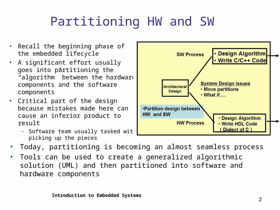
Partitioning HW and SW

• Recall the beginning phase of the embedded lifecycle

• A significant effort usually goes into partitioning the “algorithm” between the hardware components and the software components

• Critical part of the design because mistakes made here can cause an inferior product to result- Software team usually tasked with

picking up the pieces• Today, partitioning is becoming an almost seamless process• Tools can be used to create a generalized algorithmic solution (UML)

and then partitioned into software and hardware components


Partitioning: The duality of software and hardware

• The hardware and software in an embedded system work together to solve a problem ( algorithm )

• The decision about how to partition the software components and the hardware components is usually dictated by speed and cost- Dedicated hardware is fast, inflexible and expensive- Reconfigurable hardware is fast, flexible and more expensive- Software is slower, more flexible and cheaper

LASER PRINTER ENGINE

DATA TO BE PRINTED CARBON TONER ON PAPER

ALGORITHM

MECHANICALCONTROL

DATAFORMATTING

LASER CONTROL

ERROR HANDLING


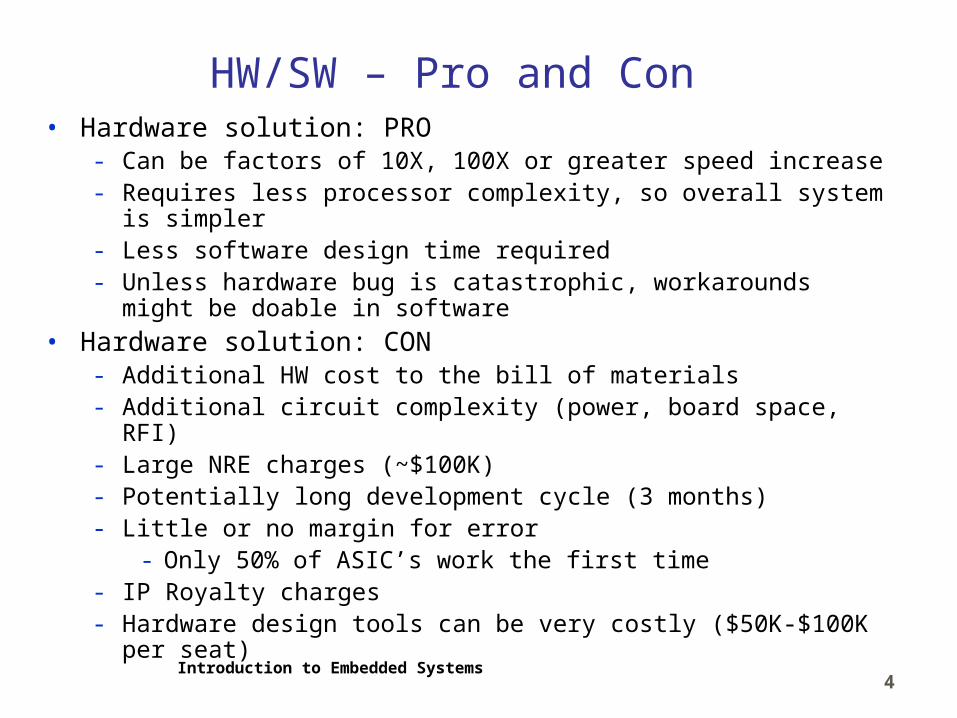
HW/SW – Pro and Con• Hardware solution: PRO

- Can be factors of 10X, 100X or greater speed increase- Requires less processor complexity, so overall system is

simpler- Less software design time required- Unless hardware bug is catastrophic, workarounds might be

doable in software• Hardware solution: CON

- Additional HW cost to the bill of materials- Additional circuit complexity (power, board space, RFI)- Large NRE charges (~$100K)- Potentially long development cycle (3 months)- Little or no margin for error

- Only 50% of ASIC’s work the first time- IP Royalty charges - Hardware design tools can be very costly ($50K-$100K per

seat)


HW/SW – Pro and Con• Software solution: PRO

- No additional impact on materials costs, power requirements, circuit complexity

- Bugs are easily dealt with, even in the field!- Software design tools are relatively inexpensive- Not sensitive to sales volumes

• Software solutions: CON- Relative performance versus hardware is generally far inferior- Additional algorithmic requirements forces more processing

power- Bigger, faster, processor(s)- More memory- Bigger power supply

- RTOS may be necessary (royalties)- More uncertainty in software development schedule- Performance goals may not be achievable in the time available- Larger software development team adds to development costs


HW/SW cost analysis example• Assume that we are

considering the addition of an ASIC to our embedded system

Annual volume

1,000 units 500,000 units

Cost per ASIC

$14.00 $6.00

Total cost $14,000 $3,000,000

• Assume that the cost of developing the ASIC can be summarized as follows:

Annual volume

1,000 units 500,000 units

Development cost (2 eng-

yrs)

$300,000 $300,000

NRE foundry charges

$200,000 $200,000

Amortized tool costs

$25,000 $25,000

Cost per device

$525 $5.25

Total cost $525,000 $525,000


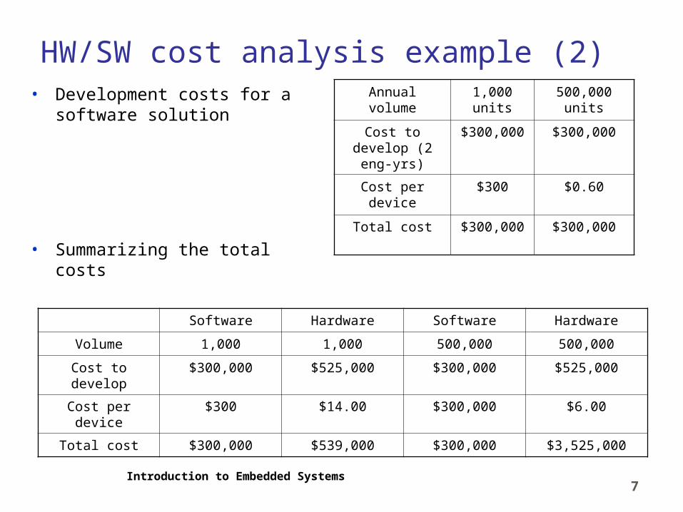
HW/SW cost analysis example (2)• Development costs for a

software solution

• Summarizing the total costs

Annual volume 1,000 units

500,000 units

Cost to develop (2 eng-yrs)

$300,000 $300,000

Cost per device

$300 $0.60

Total cost $300,000 $300,000

Software Hardware Software Hardware

Volume 1,000 1,000 500,000 500,000

Cost to develop $300,000 $525,000 $300,000 $525,000

Cost per device $300 $14.00 $300,000 $6.00

Total cost $300,000 $539,000 $300,000 $3,525,000


HW/SW cost analysis example (3)• Let’s assume that the product is an ink jet printer and that we can

judge the possible list price versus features

HW solution Software solution

Printing speed (Pages per minute)

4 1

Selling price $139 $89

• Question: What partitioning direction should we take?- Risk analysis:

- 30% probability that ASIC will require a second pass through foundry

- $200,000 + 2 months- Software teams have never come in on schedule

- Averaged 3 month overrun for last 4 projects- Consumer Electronics Show is in 4 months


Partitioning HW and Software

• There has been a revolution in hardware design called Hardware Description Languages (HDL)- Commonly known as Verilog and VHDL- Like C, but includes extensions for real time and other

hardware realities- Abstracts the design of hardware away from gates and wires

to algorithms and state machines• Hardware design is described in HDL and then compiles to

a recipe for the silicon FAB to build the circuit- Called Silicon Compilation

• A single HW designer can now develop an IC that required entire teams several years ago- This has led to whole new concept of Systems-on-a-chip, or

SOC


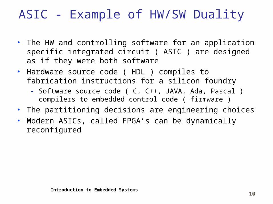
ASIC - Example of HW/SW Duality

• The HW and controlling software for an application specific integrated circuit ( ASIC ) are designed as if they were both software

• Hardware source code ( HDL ) compiles to fabrication instructions for a silicon foundry- Software source code ( C, C++, JAVA, Ada, Pascal ) compilers

to embedded control code ( firmware )

• The partitioning decisions are engineering choices• Modern ASICs, called FPGA’s can be dynamically

reconfigured

Introduction to Embedded Systems

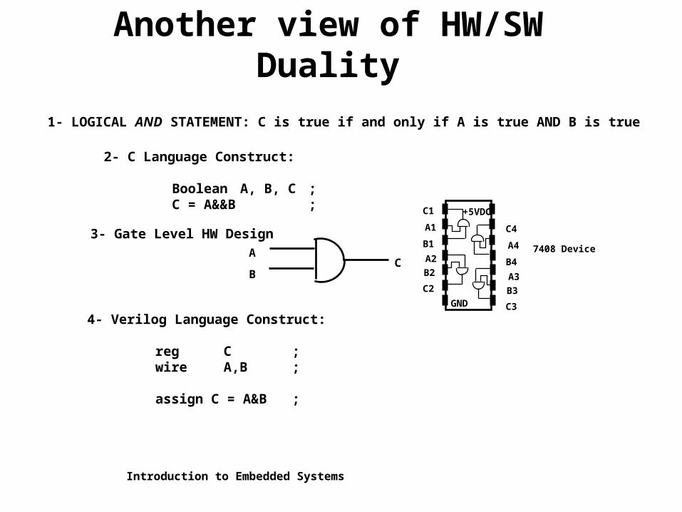
1- LOGICAL AND STATEMENT: C is true if and only if A is true AND B is true

2- C Language Construct:

Boolean A, B, C ;C = A&&B ;

A

BC

3- Gate Level HW Design

+5VDC

GND

C1

A1

B1

C2

A2

B2

C4

A4

B4

C3

A3

B3

4- Verilog Language Construct:

reg C ;wire A,B ;

assign C = A&B ;

Another view of HW/SW Duality

7408 Device


Another view of HW/SW Duality(2)


Boolean A, B, C ;

C = A&&B ;


Boolean A, B, C ;

C = A&&B ;

C Compiler/Assembler/Linker/Loader

Algorithm implements the AND function

Algorithm implements the AND function

Software Implementation


reg C ;wire A,B ;

assign C = A&B ;


reg C ;wire A,B ;

assign C = A&B ;

Verilog Compiler/IC Design Library/IC fabrication

Hardware createdTo implement AND

Hardware createdTo implement AND

Hardware Implementation


ASIC: a System-On-Chip ( SOC )

ASIC

Embedded Microprocessor

Commerciallyavailable

“devices” ( IP )

User designed elements

FIRMWARE

Analog I/O

Digital I/O


Hardware design at the gate level


Hardware design in VHDL


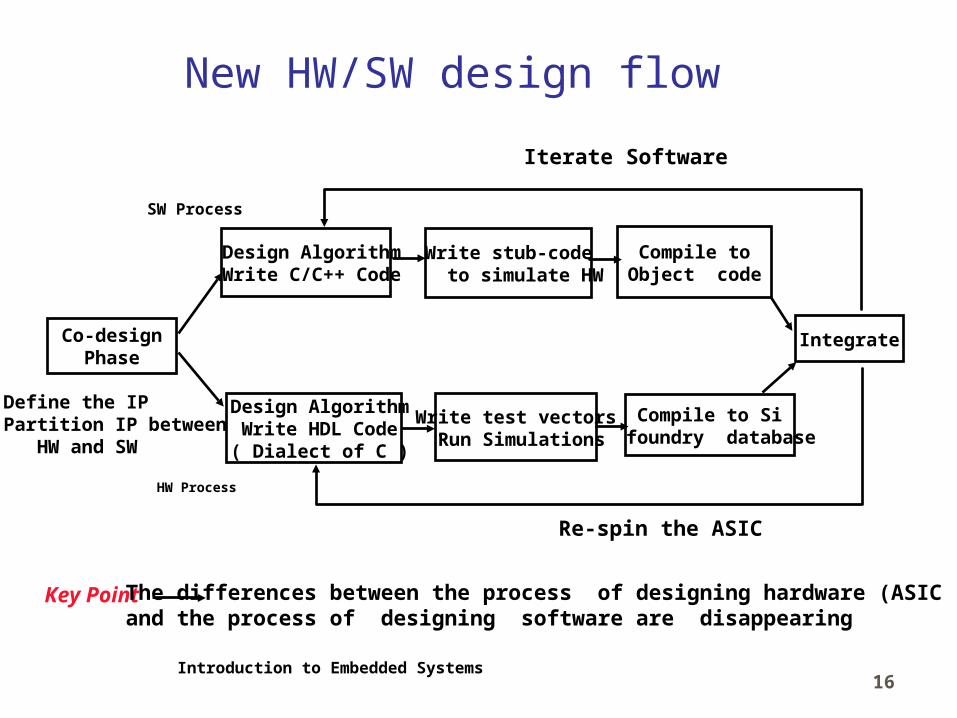
New HW/SW design flow

Co-designPhase

•Define the IP •Partition IP between HW and SW

Design Algorithm Write C/C++ Code

Design Algorithm Write HDL Code ( Dialect of C )

SW Process

HW Process

Write stub-code to simulate HW

• Write test vectors Run Simulations

Compile to Object code

Compile to Si foundry database

Integrate

Iterate Software

Re-spin the ASIC

Key Point The differences between the process of designing hardware (ASIC ) and the process of designing software are disappearing


What if…..?

• Suppose it was possible to eliminate the distinction between designing embedded hardware and embedded software

• Could focus on the algorithmic solution and let the partitioning be a natural consequence of the design

• Many of the barriers to effective development would be eliminated- No more, Throw it over the wall!

• Would design hardware and software at a higher level of abstraction

• Let’s first define Abstraction Level


Physical Hardware

Software Driver ( Firmware or BIOS )

Application

Operating System ( RTOS )

User Interface ( Command )

Abstraction layers ( software )


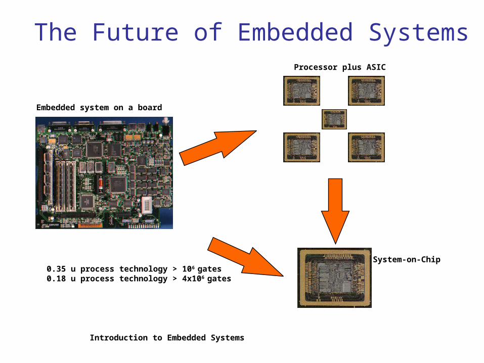
The Future of Embedded Systems

Embedded system on a board

Processor plus ASIC

System-on-Chip0.35 u process technology > 106 gates0.18 u process technology > 4x106 gates


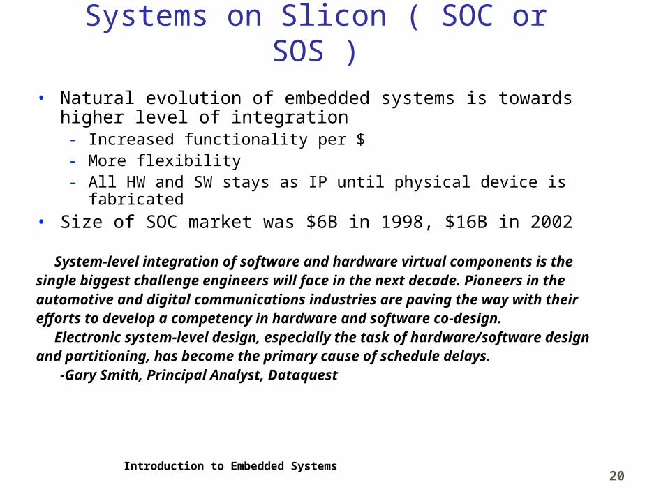
Systems on Slicon ( SOC or SOS )• Natural evolution of embedded systems is towards higher

level of integration- Increased functionality per $- More flexibility- All HW and SW stays as IP until physical device is fabricated

• Size of SOC market was $6B in 1998, $16B in 2002

System-level integration of software and hardware virtual components is the single biggest challenge engineers will face in the next decade. Pioneers in theautomotive and digital communications industries are paving the way with their efforts to develop a competency in hardware and software co-design. Electronic system-level design, especially the task of hardware/software designand partitioning, has become the primary cause of schedule delays.

-Gary Smith, Principal Analyst, Dataquest


UML and Co-design

• Two new technologies have emerged that address this desire to focus on the algorithm and not the partition- Unified Modeling Language (UML)

- iLogix, ObjecTime, Cadence, CoWare- HW/SW Codesign

- Synopsys, Mentor Graphics, VAST• UML products, such as Statemate and Rhapsody (iLogix) and

Co-design products, such as Seamless ( Mentor Graphics ) blur the distinction between hardware and software

• Output of UML tool is C++ application code and/or VHDL code- Partition decisions are made by which code is generated

• Objective: Design the algorithm in an implementation independent way- Let the automatic code generator do the grunt work


Unified Modeling Language

• UML is a way to represent the finite-state behavior of an embedded system:

A finite state machine is an abstract machine that defines a

set of conditions of existence ( called “states” ), a set of

behaviors or actions performed in each of these states, and a

set of events that cause changes in states according to a finite

and well-defined rule set.

• Consider some examples of a finite state machine- Vending machine

- Gas pump

- Flight control system


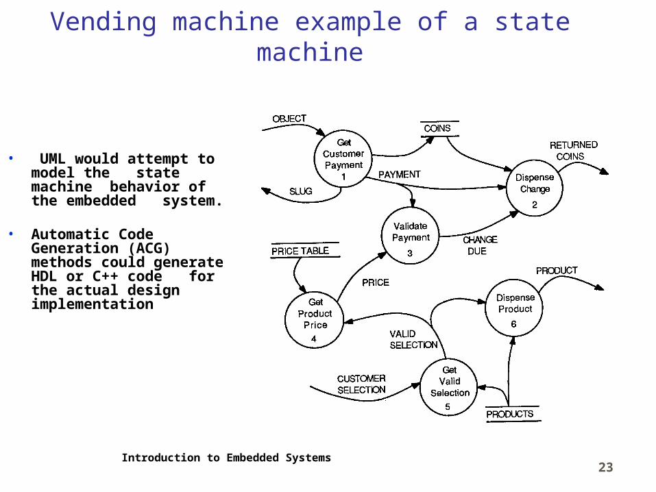
Vending machine example of a state machine

• UML would attempt to model the state machine behavior of the embedded system.

• Automatic Code Generation (ACG) methods could generate HDL or C++ code for the actual design implementation


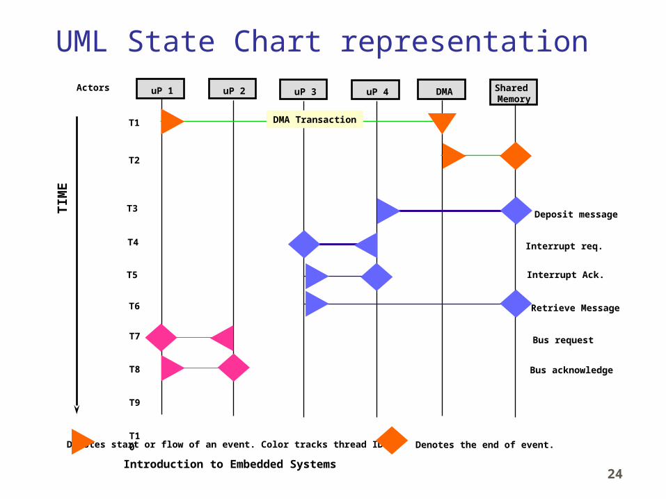
uP 1 uP 2 uP 3 uP 4 DMA Shared Memory

TIM

E

T1

T2

DMA Transaction

Deposit message

Interrupt req.

Interrupt Ack.

Retrieve Message

T3

T4

T5

T6

Actors

Denotes start or flow of an event. Color tracks thread ID. Denotes the end of event.

T7

T8

T9

T10

Bus request

Bus acknowledge

UML State Chart representation


Codevelopment design flow

Co-designPhase

•Define the IP •Partition IP between HW and SW

SW Process

HW Process

• Design Algorithm• Write C/C++ Code

• Design Algorithm• Write HDL Code ( Dialect of C )

• Write test vectors• Run Simulations

• Write stub-code to simulate HW

• Compile to Object code

•Compile to Si foundry database

Integrate

Iterate Software

Re-spin the ASIC

Key Point The distinctions between the process of designing hardware and the process of designing software are blurring

Co-verification• Exercise SW• Generate Vectors• Validate Interfaces

System Design• Move partitions• What if….•Simulate bus loading


Typical Embedded System Design Cycle

Architect & Specify

Software Development

Hardware Development

ProtosProtos Integrate & Test

•Spreadsheets•C Models•Domain - Specific ESDA Tools

•EDA SW Tools•ASIC Emulators

•Debuggers•Compilers•RTOS

•In-Circuit Emulators•ROM Monitors

•Post-release support tools??

Maintenance

Enhancement


HW/SW Co-verification• After a design is partitioned and separate HW and SW

development is proceeding, how do you know that you’ll get it right?- Re-spinning an ASIC is costly- Fixing a problem in software will reduce performance

• HW/SW Co-verification focuses on validating the correctness of the design across the HW/SW interface


Where design time is spent

SystemSpecification

& Design

HW & SWDesign/Debug

PrototypeDebug

Source: Dataquest Cost to fixa problem

12%37% 20% 31%

51% of Time51% of Time

SystemTest

Maintenance and upgrade


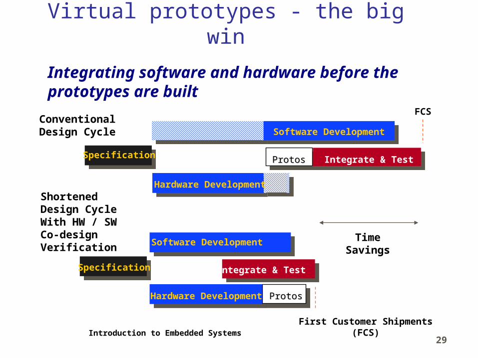
Virtual prototypes - the big win

TimeSavings

ShortenedDesign CycleWith HW / SWCo-design Verification

Specification

ConventionalDesign Cycle



Integrate & Test

FCS

First Customer Shipments(FCS)

Integrate & Test



Specification

ProtosProtos

ProtosProtos

Integrating software and hardware before the prototypes are built


Incremental HW/SW IntegrationSpecification

Partition

Develop Algorithms HDL

Develop Algorithms C or C++

Early iterations

Unit testing - Vectors Unit testing - Stub code

HW System Simulate

Integration

Synthesis/Layout/Fab Team builds object code

Fix it in SWASIC Spin

Maintenance & upgrade

“SW team is done”

Co

-ve

rifi

ca

tio

n


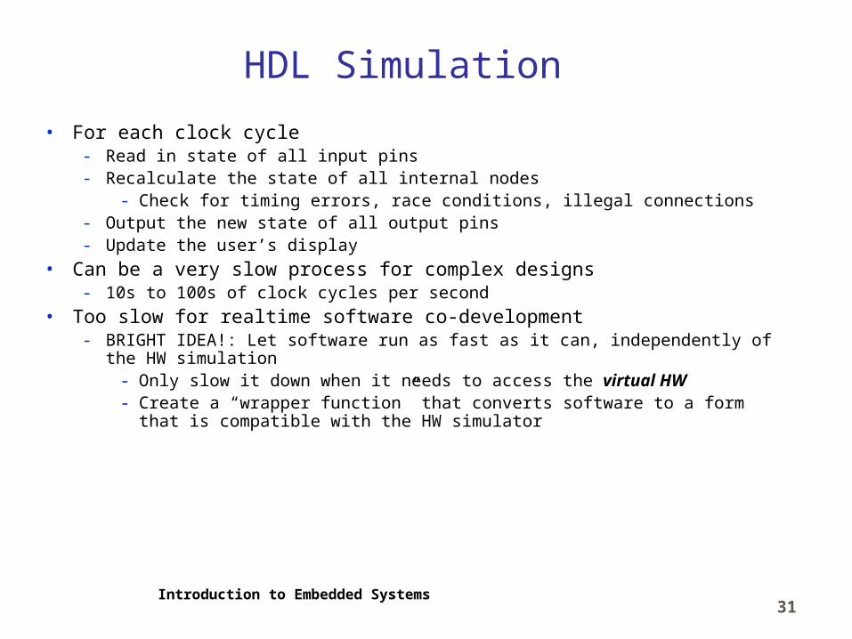
HDL Simulation

• For each clock cycle- Read in state of all input pins- Recalculate the state of all internal nodes

- Check for timing errors, race conditions, illegal connections- Output the new state of all output pins- Update the user’s display

• Can be a very slow process for complex designs- 10s to 100s of clock cycles per second

• Too slow for realtime software co-development- BRIGHT IDEA!: Let software run as fast as it can, independently of the HW

simulation- Only slow it down when it needs to access the virtual HW- Create a “wrapper function” that converts software to a form that is

compatible with the HW simulator


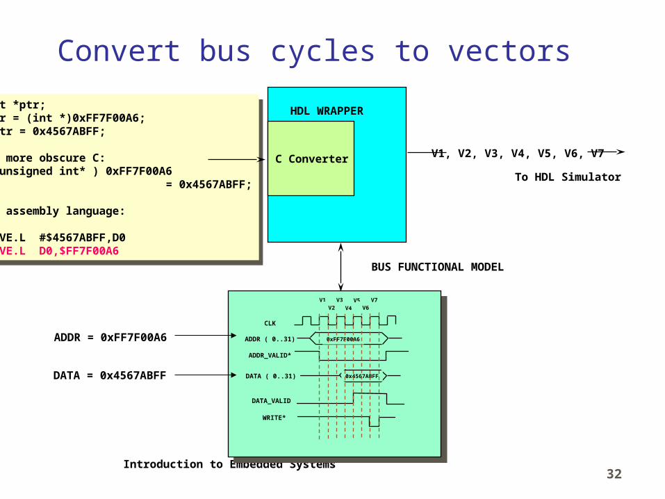
Convert bus cycles to vectors

HDL WRAPPER

BUS FUNCTIONAL MODEL

C Converter V1, V2, V3, V4, V5, V6, V7

To HDL Simulator

int *ptr;ptr = (int *)0xFF7F00A6;*ptr = 0x4567ABFF;

Or more obscure C:*(unsigned int* ) 0xFF7F00A6 = 0x4567ABFF;

or assembly language:

MOVE.L #$4567ABFF,D0MOVE.L D0,$FF7F00A6

int *ptr;ptr = (int *)0xFF7F00A6;*ptr = 0x4567ABFF;

Or more obscure C:*(unsigned int* ) 0xFF7F00A6 = 0x4567ABFF;

or assembly language:

MOVE.L #$4567ABFF,D0MOVE.L D0,$FF7F00A6

CLK

ADDR ( 0..31) 0xFF7F00A6

ADDR_VALID*

DATA ( 0..31) 0x4567ABFF

DATA_VALID

WRITE*

V1V2

V3

V4

V5V6

V7

ADDR = 0xFF7F00A6

DATA = 0x4567ABFF


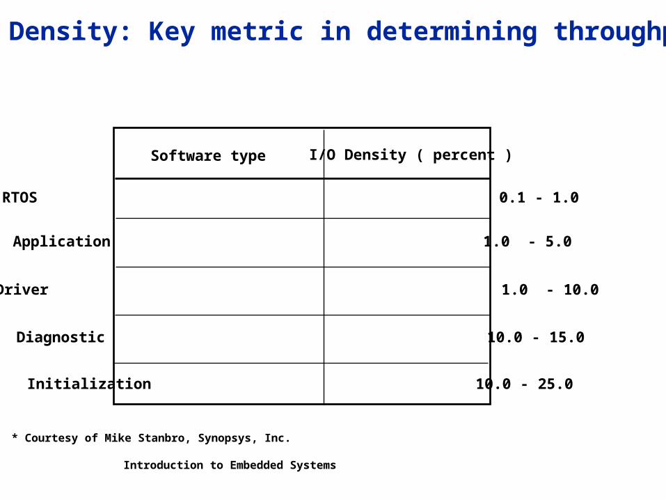
Software type I/O Density ( percent )

RTOS 0.1 - 1.0

Application 1.0 - 5.0

Driver 1.0 - 10.0

Diagnostic 10.0 - 15.0

Initialization 10.0 - 25.0

I/O Density: Key metric in determining throughput*

* Courtesy of Mike Stanbro, Synopsys, Inc.


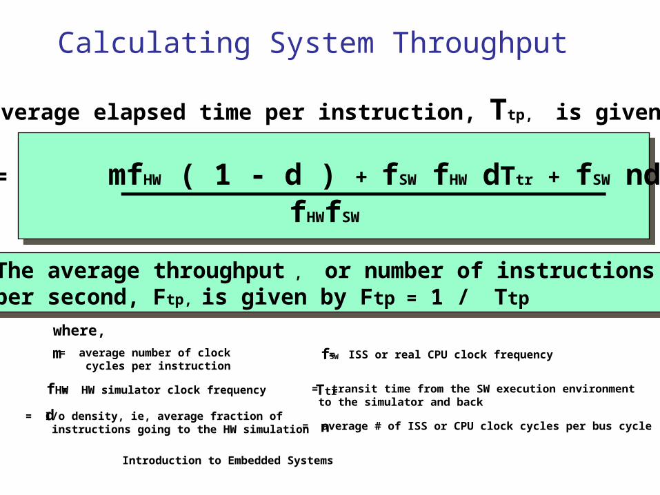
Calculating System Throughput

Ttp = mfHW ( 1 - d ) + fSW fHW dTtr + fSW ndfHWfSW

The average elapsed time per instruction, Ttp, is given by:

The average throughput , or number of instructions per second, Ftp, is given by Ftp = 1 / Ttp

The average throughput , or number of instructions per second, Ftp, is given by Ftp = 1 / Ttp

= HW simulator clock frequencyfHW

= I/o density, ie, average fraction of instructions going to the HW simulation

d

= transit time from the SW execution environment to the simulator and back

Ttr

= ISS or real CPU clock frequencyfSW = average number of clock cycles per instruction

m

= average # of ISS or CPU clock cycles per bus cyclen

where,


1.00E+03

1.00E+04

1.00E+05

1.00E+06

1.00E+07

0.001,HW =

100 Hz

0.002,HW =

100 Hz

0.005,HW =

100 Hz

0.010,HW =

100 Hz

0.020,HW =

100 Hz

0.050,HW =

100 Hz

0

5000

10000

15000

20000

25000

30000

35000

40000

Th

rou

gh

pu

t (

inst

ruct

ion

s p

er s

eco

nd

)

ISS or CPU Clock Speed ( Hz )

I/O Density

Throughput as a Function of Software Clock Speed and I/O Density for Remote Call Latency = 0.005 sec and HW Simulation Rate = 100 Hz

Low I/O Density View

35000-40000

30000-35000

25000-30000

20000-25000

15000-20000

10000-15000

5000-10000

0-5000

Plotting the results in Excel


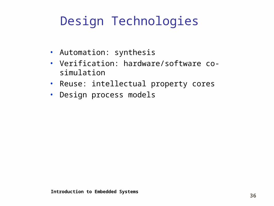
Design Technologies

• Automation: synthesis• Verification: hardware/software co-simulation• Reuse: intellectual property cores• Design process models


Introduction• Design task

- Define system functionality- Convert functionality to physical implementation while

- Satisfying constrained metrics- Optimizing other design metrics

• Designing embedded systems is hard- Complex functionality

- Millions of possible environment scenarios- Competing, tightly constrained metrics

- Productivity gap- As low as 10 lines of code or 100 transistors produced per

day


Improving productivity

• Design technologies developed to improve productivity• We focus on technologies advancing hardware/software

unified view- Automation

- Program replaces manual design- Synthesis

- Reuse- Predesigned components- Cores- General-purpose and single-purpose processors on single

IC- Verification

- Ensuring correctness/completeness of each design step- Hardware/software co-simulation

Reuse

Specification

Implementation

Automation

Verification


Automation: synthesis

• Early design mostly hardware• Software complexity increased with

advent of general-purpose processor• Different techniques for software design

and hardware design - Caused division of the two fields

• Design tools evolve for higher levels of abstraction

- Different rate in each field• Hardware/software design fields

rejoining- Both can start from behavioral

description in sequential program model- 30 years longer for hardware design to

reach this step in the ladder- Many more design dimensions- Optimization critical Implementation

Assembly instructions

Machine instructions Logic gates

Logic equations / FSM's

Register transfers

Sequential program code (e.g., C, VHDL)

Compilers(1960s,1970s)

Assemblers, linkers(1950s, 1960s)

Behavioral synthesis(1990s)

RT synthesis(1980s, 1990s)

Logic synthesis(1970s, 1980s)

Microprocessor plus program bits

VLSI, ASIC, or PLD implementation

The codesign ladder


Hardware/software parallel evolution

• Software design evolution- Machine instructions- Assemblers

- convert assembly programs into machine instructions

- Compilers - translate sequential programs

into assembly• Hardware design evolution

- Interconnected logic gates- Logic synthesis

- converts logic equations or FSMs into gates

- Register-transfer (RT) synthesis - converts FSMDs into FSMs, logic

equations, predesigned RT components (registers, adders, etc.)

- Behavioral synthesis- converts sequential programs

into FSMDs

Implementation

Assembly instructions

Machine instructions Logic gates

Logic equations / FSM's

Register transfers

Sequential program code (e.g., C, VHDL)

Compilers(1960s,1970s)

Assemblers, linkers(1950s, 1960s)

Behavioral synthesis(1990s)

RT synthesis(1980s, 1990s)

Logic synthesis(1970s, 1980s)

Microprocessor plus program bits

VLSI, ASIC, or PLD implementation

The codesign ladder


Increasing abstraction level

• Higher abstraction level focus of hardware/software design evolution- Description smaller/easier to capture

- E.g., Line of sequential program code can translate to 1000 gates- Many more possible implementations available

- (a) Like flashlight, the higher above the ground, the more ground illuminated- Sequential program designs may differ in performance/transistor count by

orders of magnitude- Logic-level designs may differ by only power of 2

- (b) Design process proceeds to lower abstraction level, narrowing in on single implementation

(a) (b)

idea

implementation

back-of-the-envelope

sequential programregister-transfers

logic

mod

elin

g co

st in

crea

ses

oppo

rtun

itie

s de

crea

se

idea

implementation


Synthesis

• Automatically converting system’s behavioral description to a structural implementation

- Complex whole formed by parts- Structural implementation must optimize design metrics

• More expensive, complex than compilers- Cost = $100s to $10,000s- User controls 100s of synthesis options- Optimization critical

- Otherwise could use software- Optimizations different for each user- Run time = hours, days


Gajski’s Y-chart

• Each axis represents type of description- Behavioral

- Defines outputs as function of inputs- Algorithms but no implementation

- Structural- Implements behavior by connecting

components with known behavior- Physical

- Gives size/locations of components and wires on chip/board

• Synthesis converts behavior at given level to structure at same level or lower

- E.g.,- FSM → gates, flip-flops (same level)- FSM → transistors (lower level)- FSM X registers, FUs (higher level)- FSM X processors, memories (higher

level)

Behavior

Physical

Structural

Processors, memories

Registers, FUs, MUXs

Gates, flip-flops

Transistors

Sequential programs

Register transfers

Logic equations/FSM

Transfer functions

Cell Layout

Modules

Chips

Boards


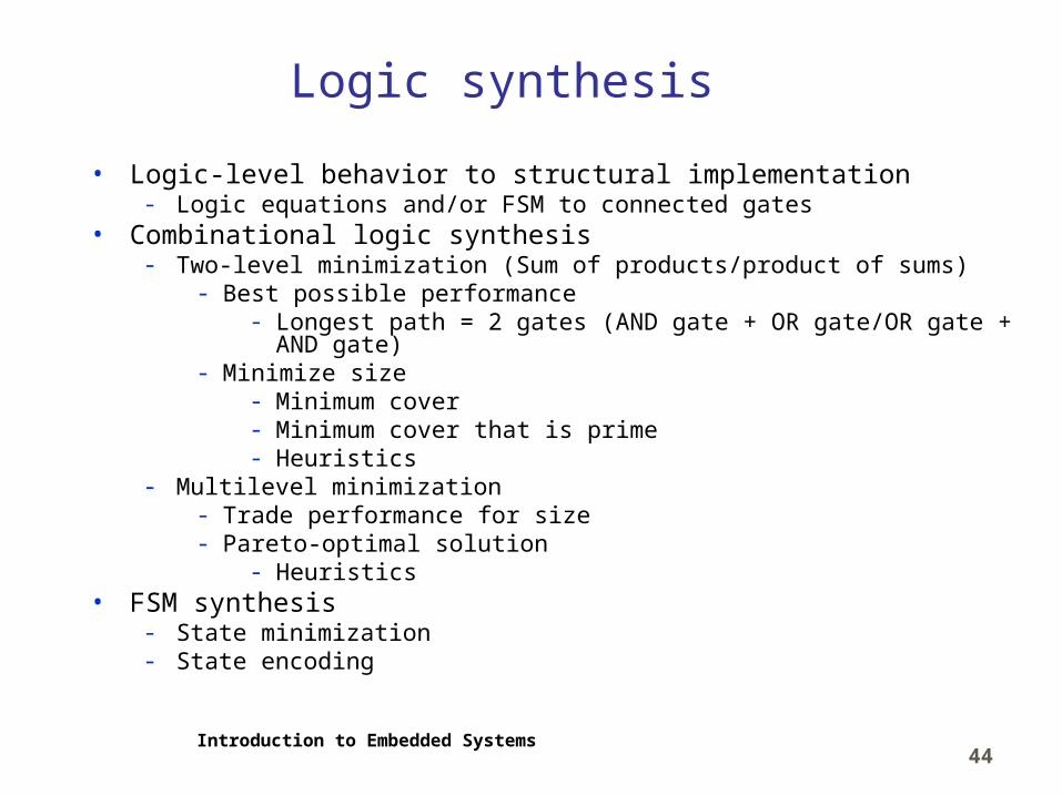
Logic synthesis

• Logic-level behavior to structural implementation- Logic equations and/or FSM to connected gates

• Combinational logic synthesis- Two-level minimization (Sum of products/product of sums)

- Best possible performance- Longest path = 2 gates (AND gate + OR gate/OR gate + AND

gate)- Minimize size

- Minimum cover- Minimum cover that is prime- Heuristics

- Multilevel minimization- Trade performance for size- Pareto-optimal solution

- Heuristics• FSM synthesis

- State minimization- State encoding


Two-level minimization• Represent logic function as sum of products

(or product of sums)- AND gate for each product- OR gate for each sum

• Gives best possible performance- At most 2 gate delay

• Goal: minimize size- Minimum cover

- Minimum # of AND gates (sum of products)

- Minimum cover that is prime- Minimum # of inputs to each AND gate

(sum of products)

F = abc'd' + a'b'cd + a'bcd + ab'cd

Sum of products

4 4-input AND gates and 1 4-input OR gate

→ 40 transistors

a

b

c

d

F

Direct implementation


Minimum cover

• Minimum # of AND gates (sum of products)• Literal: variable or its complement

- a or a’, b or b’, etc.

• Minterm: product of literals- Each literal appears exactly once

- abc’d’, ab’cd, a’bcd, etc.

• Implicant: product of literals- Each literal appears no more than once

- abc’d’, a’cd, etc.- Covers 1 or more minterms

- a’cd covers a’bcd and a’b’cd

• Cover: set of implicants that covers all minterms of function• Minimum cover: cover with minimum # of implicants


Minimum cover: K-map approach

• Karnaugh map (K-map)- 1 represents minterm- Circle represents implicant

• Minimum cover- Covering all 1’s with min # of

circles- Example: direct vs. min cover

- Less gates- 4 vs. 5

- Less transistors- 28 vs. 40

11

10 0 0

0 0 1 0

1 0 0 0

0 0 0

abcd

00

01

11

10

00 01 10

1

10 0 0

0 0 1 0

1 0 0 0

0 0 0

abcd

00

01

11

10

00 01 11 10

1

F=abc'd' + a'cd + ab'cd

a

bc

d

F

2 4-input AND gate1 3-input AND gates1 4 input OR gate → 28 transistors

K-map: sum of products K-map: minimum cover

Minimum cover

Minimum cover implementation


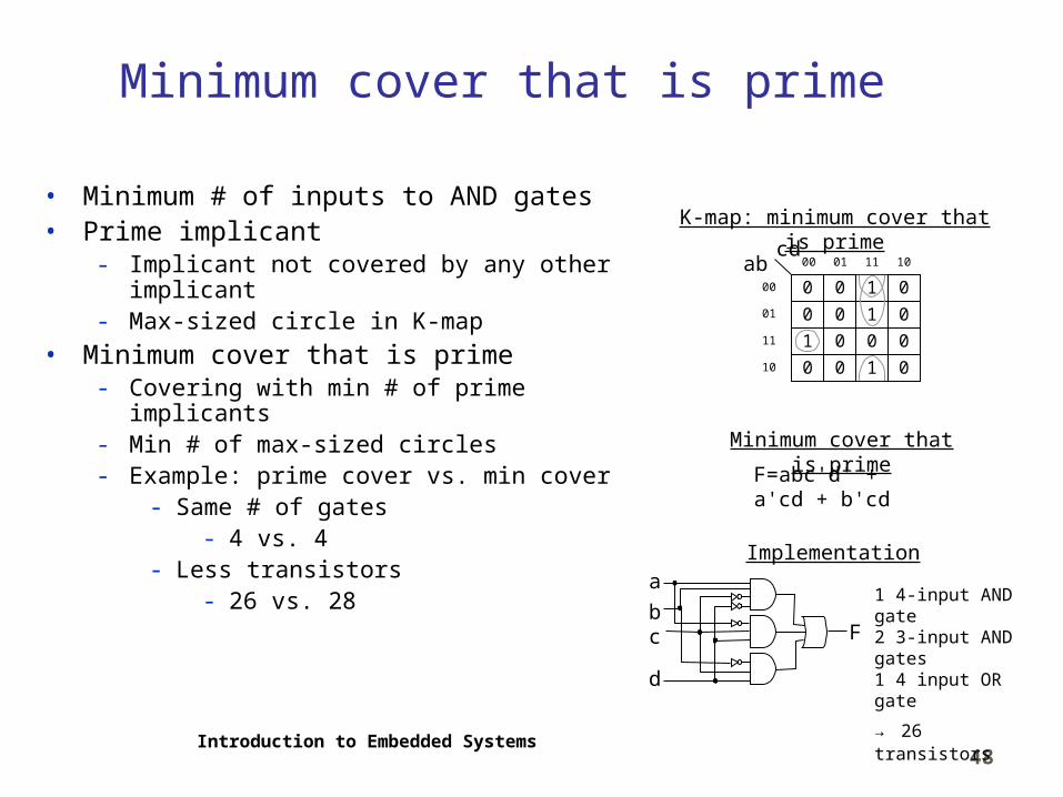
Minimum cover that is prime

• Minimum # of inputs to AND gates• Prime implicant

- Implicant not covered by any other implicant

- Max-sized circle in K-map• Minimum cover that is prime

- Covering with min # of prime implicants- Min # of max-sized circles- Example: prime cover vs. min cover

- Same # of gates- 4 vs. 4

- Less transistors- 26 vs. 28

10 0 0

0 0 1 0

1 0 0 0

0 0 0

abcd

00

01

11

10

00 01 11 10

1

K-map: minimum cover that is prime

Minimum cover that is prime

F=abc'd' + a'cd + b'cd

1 4-input AND gate 2 3-input AND gates1 4 input OR gate

→ 26 transistors

F

a

bc

d

Implementation


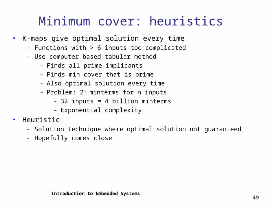
Minimum cover: heuristics• K-maps give optimal solution every time

- Functions with > 6 inputs too complicated- Use computer-based tabular method

- Finds all prime implicants- Finds min cover that is prime- Also optimal solution every time- Problem: 2n minterms for n inputs

- 32 inputs = 4 billion minterms- Exponential complexity

• Heuristic- Solution technique where optimal solution not guaranteed- Hopefully comes close


Heuristics: iterative improvement

• Start with initial solution- i.e., original logic equation

• Repeatedly make modifications toward better solution• Common modifications

- Expand- Replace each nonprime implicant with a prime implicant covering it- Delete all implicants covered by new prime implicant

- Reduce- Opposite of expand

- Reshape- Expands one implicant while reducing another- Maintains total # of implicants

- Irredundant- Selects min # of implicants that cover from existing implicants

• Synthesis tools differ in modifications used and the order they are used


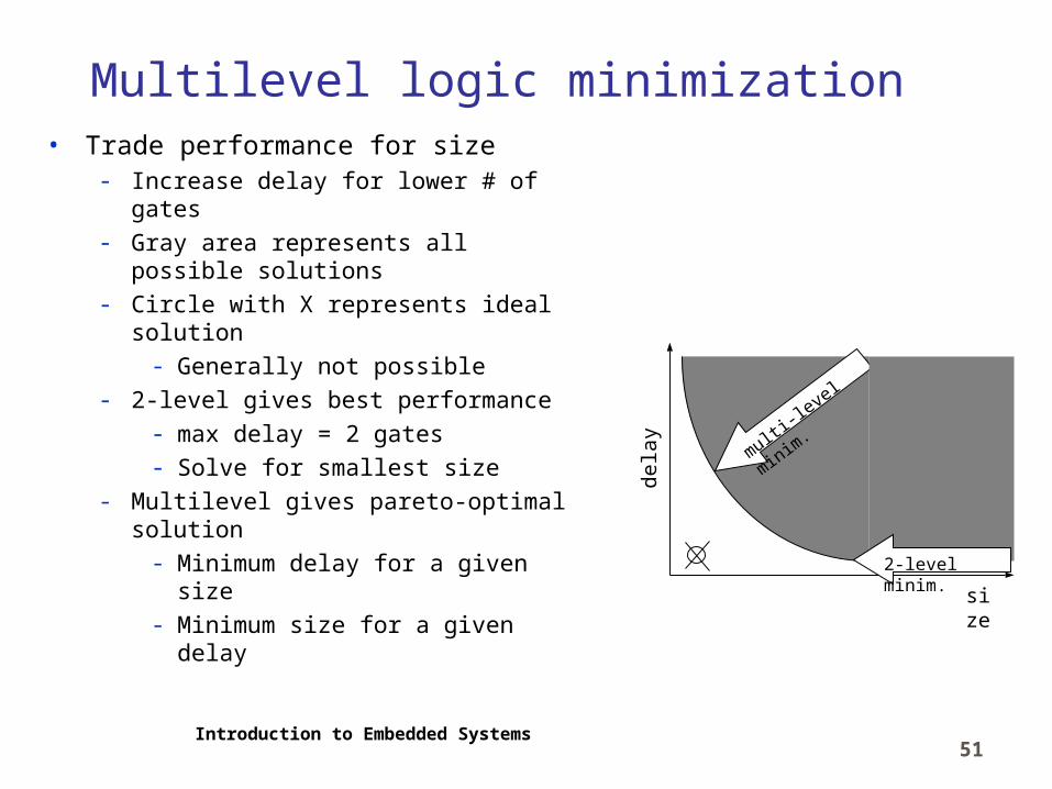
Multilevel logic minimization• Trade performance for size

- Increase delay for lower # of gates- Gray area represents all possible

solutions- Circle with X represents ideal solution

- Generally not possible- 2-level gives best performance

- max delay = 2 gates- Solve for smallest size

- Multilevel gives pareto-optimal solution

- Minimum delay for a given size- Minimum size for a given delay

size

dela

y

multi-lev

el minim

.

2-level minim.


Example• Minimized 2-level logic function:

- F = adef + bdef + cdef + gh- Requires 5 gates with 18 total gate inputs

- 4 ANDS and 1 OR• After algebraic manipulation:

- F = (a + b + c)def + gh- Requires only 4 gates with 11 total gate inputs

- 2 ANDS and 2 ORs- Less inputs per gate- Assume gate inputs = 2 transistors

- Reduced by 14 transistors- 36 (18 * 2) down to 22 (11 * 2)

- Sacrifices performance for size- Inputs a, b, and c now have 3-gate delay

• Iterative improvement heuristic commonly used

F

b

ce

a

d

fgh

2-level minimized

F

bc

e

a

d

fgh

multilevel minimized


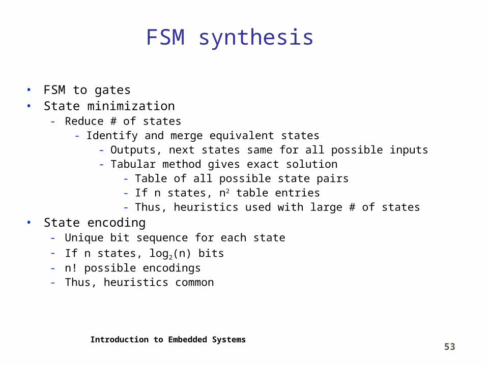
FSM synthesis

• FSM to gates• State minimization

- Reduce # of states- Identify and merge equivalent states

- Outputs, next states same for all possible inputs- Tabular method gives exact solution

- Table of all possible state pairs- If n states, n2 table entries- Thus, heuristics used with large # of states

• State encoding- Unique bit sequence for each state- If n states, log2(n) bits- n! possible encodings- Thus, heuristics common


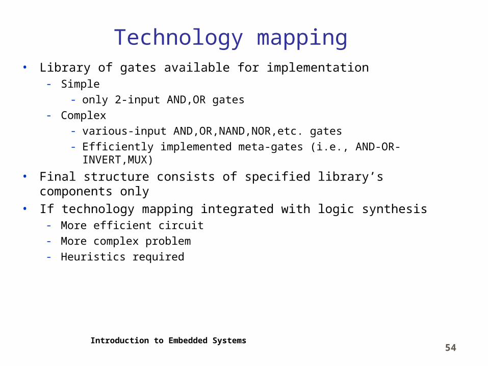
Technology mapping• Library of gates available for implementation

- Simple- only 2-input AND,OR gates

- Complex- various-input AND,OR,NAND,NOR,etc. gates- Efficiently implemented meta-gates (i.e., AND-OR-INVERT,MUX)

• Final structure consists of specified library’s components only• If technology mapping integrated with logic synthesis

- More efficient circuit- More complex problem- Heuristics required


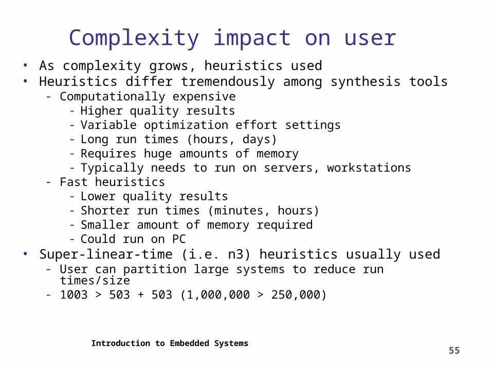
Complexity impact on user• As complexity grows, heuristics used• Heuristics differ tremendously among synthesis tools

- Computationally expensive- Higher quality results- Variable optimization effort settings- Long run times (hours, days)- Requires huge amounts of memory- Typically needs to run on servers, workstations

- Fast heuristics- Lower quality results- Shorter run times (minutes, hours)- Smaller amount of memory required- Could run on PC

• Super-linear-time (i.e. n3) heuristics usually used- User can partition large systems to reduce run times/size- 1003 > 503 + 503 (1,000,000 > 250,000)


Integrating logic design and physical design

• Past- Gate delay much greater than wire

delay- Thus, performance evaluated as # of

levels of gates only

• Today- Gate delay shrinking as feature size

shrinking- Wire delay increasing

- Performance evaluation needs wire length

- Transistor placement (needed for wire length) domain of physical design

- Thus, simultaneous logic synthesis and physical design required for efficient circuits

Wire

Transistor

Del

ay

Reduced feature size


Register-transfer synthesis

• Converts FSMD to custom single-purpose processor- Datapath

- Register units to store variables- Complex data types

- Functional units- Arithmetic operations

- Connection units- Buses, MUXs

- FSM controller- Controls datapath

- Key sub problems:- Allocation

- Instantiate storage, functional, connection units- Binding

- Mapping FSMD operations to specific units


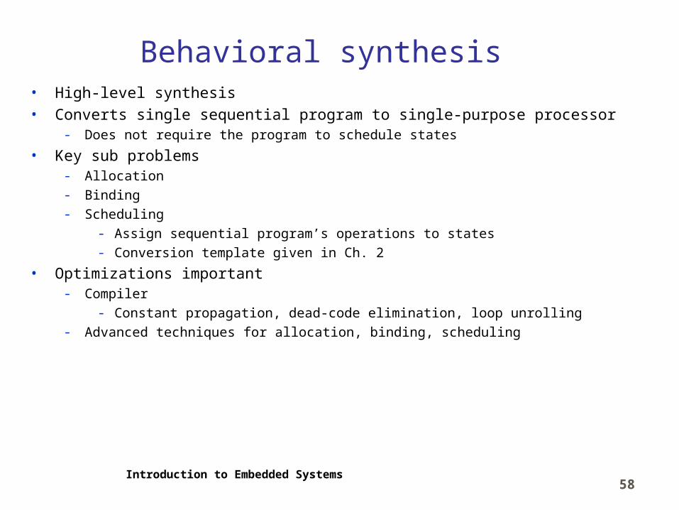
Behavioral synthesis• High-level synthesis• Converts single sequential program to single-purpose processor

- Does not require the program to schedule states

• Key sub problems- Allocation- Binding- Scheduling

- Assign sequential program’s operations to states- Conversion template given in Ch. 2

• Optimizations important- Compiler

- Constant propagation, dead-code elimination, loop unrolling- Advanced techniques for allocation, binding, scheduling


System synthesis• Convert 1 or more processes into 1 or more processors (system)

- For complex embedded systems- Multiple processes may provide better performance/power- May be better described using concurrent sequential programs

• Tasks- Transformation

- Can merge 2 exclusive processes into 1 process- Can break 1 large process into separate processes- Procedure inlining- Loop unrolling

- Allocation- Essentially design of system architecture

- Select processors to implement processes- Also select memories and busses


System synthesis• Tasks (cont.)

- Partitioning- Mapping 1 or more processes to 1 or more processors- Variables among memories- Communications among buses

- Scheduling- Multiple processes on a single processor- Memory accesses- Bus communications

- Tasks performed in variety of orders- Iteration among tasks common


System synthesis• Synthesis driven by constraints

- E.g.,- Meet performance requirements at minimum cost

- Allocate as much behavior as possible to general-purpose processor- Low-cost/flexible implementation

- Minimum # of SPPs used to meet performance

• System synthesis for GPP only (software)- Common for decades

- Multiprocessing- Parallel processing- Real-time scheduling

• Hardware/software codesign- Simultaneous consideration of GPPs/SPPs during synthesis- Made possible by maturation of behavioral synthesis in 1990’s


Temporal vs. spatial thinking• Design thought process changed by evolution of synthesis• Before synthesis

- Designers worked primarily in structural domain- Connecting simpler components to build more complex systems

- Connecting logic gates to build controller- Connecting registers, MUXs, ALUs to build datapath

- “capture and simulate” era- Capture using CAD tools- Simulate to verify correctness before fabricating

- Spatial thinking- Structural diagrams- Data sheets


Temporal vs. spatial thinking• After synthesis

- “describe-and-synthesize” era- Designers work primarily in behavioral domain- “describe and synthesize” era

- Describe FSMDs or sequential programs- Synthesize into structure

- Temporal thinking- States or sequential statements have relationship over time

• Strong understanding of hardware structure still important- Behavioral description must synthesize to efficient structural

implementation


Verification • Ensuring design is correct and complete

- Correct- Implements specification accurately

- Complete- Describes appropriate output to all relevant input

• Formal verification- Hard- For small designs or verifying certain key properties only

• Simulation- Most common verification method


Formal verification• Analyze design to prove or disprove certain properties• Correctness example

- Prove ALU structural implementation equivalent to behavioral description

- Derive Boolean equations for outputs- Create truth table for equations- Compare to truth table from original behavior

• Completeness example- Formally prove elevator door can never open while elevator is moving

- Derive conditions for door being open- Show conditions conflict with conditions for elevator moving


Simulation• Create computer model of design

- Provide sample input- Check for acceptable output

• Correctness example- ALU

- Provide all possible input combinations- Check outputs for correct results

• Completeness example- Elevator door closed when moving

- Provide all possible input sequences- Check door always closed when elevator moving


Increases confidence

• Simulating all possible input sequences impossible for most systems- E.g., 32-bit ALU

- 232 * 232 = 264 possible input combinations- At 1 million combinations/sec- ½ million years to simulate- Sequential circuits even worse

• Can only simulate tiny subset of possible inputs- Typical values- Known boundary conditions

- E.g., 32-bit ALU- Both operands all 0’s- Both operands all 1’s

• Increases confidence of correctness/completeness• Does not prove


Advantages over physical implementation

• Controllability- Control time

- Stop/start simulation at any time- Control data values

- Inputs or internal values

• Observability- Examine system/environment values at any time

• Debugging- Can stop simulation at any point and:

- Observe internal values- Modify system/environment values before restarting

- Can step through small intervals (i.e., 500 nanoseconds)


Disadvantages

• Simulation setup time- Often has complex external environments- Could spend more time modeling environment than system

• Models likely incomplete- Some environment behavior undocumented if complex environment- May not model behavior correctly

• Simulation speed much slower than actual execution- Sequentializing parallel design

- IC: gates operate in parallel- Simulation: analyze inputs, generate outputs for each gate 1 at time

- Several programs added between simulated system and real hardware- 1 simulated operation:

- = 10 to 100 simulator operations- = 100 to 10,000 operating system operations- = 1,000 to 100,000 hardware operations


Simulation speed• Relative speeds of different types of simulation/emulation

- 1 hour actual execution of SOC- = 1.2 years instruction-set simulation- = 10,000,000 hours gate-level simulation

10,000,000 gate-level HDL simulation

register-transfer-level HDL simulation

cycle-accurate simulation

instruction-set simulation

throughput modelhardware emulation

FPGA 1 day

1 hour

4 days

1

10

100

1000

10000

100,000

1,000,000

IC

1.4 months

1.2 years

12 years

>1 lifetime

1 millennium


Overcoming long simulation time• Reduce amount of real time simulated

- 1 msec execution instead of 1 hour- 0.001sec * 10,000,000 = 10,000 sec = 3 hours

- Reduced confidence- 1 msec of cruise controller operation tells us little

• Faster simulator- Emulators

- Special hardware for simulations- Less precise/accurate simulators

- Exchange speed for observability/controllability


Reducing precision/accuracy• Don’t need gate-level analysis for all simulations

- E.g., cruise control- Don’t care what happens at every input/output of each logic gate

- Simulating RT components ~10x faster- Cycle-based simulation ~100x faster

- Accurate at clock boundaries only- No information on signal changes between boundaries

• Faster simulator often combined with reduction in real time- If willing to simulate for 10 hours

- Use instruction-set simulator- Real execution time simulated

- 10 hours * 1 / 10,000- = 0.001 hour- = 3.6 seconds


Hardware/software co-simulation• Variety of simulation approaches exist

- From very detailed- E.g., gate-level model

- To very abstract- E.g., instruction-level model

• Simulation tools evolved separately for hardware/software- Recall separate design evolution- Software (GPP)

- Typically with instruction-set simulator (ISS)- Hardware (SPP)

- Typically with models in HDL environment• Integration of GPP/SPP on single IC creating need for merging

simulation tools


Integrating GPP/SPP simulations• Simple/naïve way

- HDL model of microprocessor- Runs system software- Much slower than ISS- Less observable/controllable than ISS

- HDL models of SPPs- Integrate all models

• Hardware-software co-simulator- ISS for microprocessor- HDL model for SPPs- Create communication between simulators- Simulators run separately except when transferring data- Faster- Though, frequent communication between ISS and HDL model slows it down


Minimizing communication• Memory shared between GPP and SPPs

- Where should memory go?- In ISS

- HDL simulator must stall for memory access- In HDL?

- ISS must stall when fetching each instruction

• Model memory in both ISS and HDL- Most accesses by each model unrelated to other’s accesses

- No need to communicate these between models- Co-simulator ensures consistency of shared data- Huge speedups (100x or more) reported with this technique


Emulators• General physical device system mapped to

- Microprocessor emulator- Microprocessor IC with some monitoring, control circuitry

- SPP emulator- FPGAs (10s to 100s)

- Usually supports debugging tasks• Created to help solve simulation disadvantages

- Mapped relatively quickly- Hours, days

- Can be placed in real environment- No environment setup time- No incomplete environment

- Typically faster than simulation- Hardware implementation


Disadvantages• Still not as fast as real implementations

- E.g., emulated cruise-control may not respond fast enough to keep control of car

• Mapping still time consuming- E.g., mapping complex SOC to 10 FPGAs

- Just partitioning into 10 parts could take weeks• Can be very expensive

- Top-of-the-line FPGA-based emulator: $100,000 to $1mill- Leads to resource bottleneck

- Can maybe only afford 1 emulator- Groups wait days, weeks for other group to finish using


Reuse: intellectual property cores• Commercial off-the-shelf (COTS) components

- Predesigned, prepackaged ICs- Implements GPP or SPP- Reduces design/debug time- Have always been available

• System-on-a-chip (SOC)- All components of system implemented on single chip- Made possible by increasing IC capacities- Changing the way COTS components sold

- As intellectual property (IP) rather than actual IC- Behavioral, structural, or physical descriptions- Processor-level components known as cores

- SOC built by integrating multiple descriptions


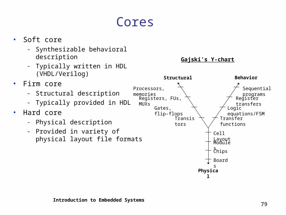
Cores• Soft core

- Synthesizable behavioral description

- Typically written in HDL (VHDL/Verilog)

• Firm core- Structural description- Typically provided in HDL

• Hard core- Physical description- Provided in variety of physical

layout file formats

Behavior

Physical

Structural

Processors, memories

Registers, FUs, MUXs

Gates, flip-flops

Transistors

Sequential programs

Register transfers

Logic equations/FSM

Transfer functions

Cell Layout

Modules

Chips

Boards

Gajski’s Y-chart


Advantages/disadvantages of hard core• Ease of use

- Developer already designed and tested core- Can use right away- Can expect to work correctly

• Predictability- Size, power, performance predicted accurately

• Not easily mapped (retargeted) to different process- E.g., core available for vendor X’s 0.25 micrometer CMOS

process- Can’t use with vendor X’s 0.18 micrometer process- Can’t use with vendor Y


Advantages/disadvantages of soft/firm cores

• Soft cores- Can be synthesized to nearly any technology- Can optimize for particular use

- E.g., delete unused portion of core- Lower power, smaller designs

- Requires more design effort- May not work in technology not tested for- Not as optimized as hard core for same processor

• Firm cores- Compromise between hard and soft cores

- Some retargetability- Limited optimization- Better predictability/ease of use


New challenges to processor providers

• Cores have dramatically changed business model- Pricing models

- Past- Vendors sold product as IC to designers- Designers must buy any additional copies

- Could not (economically) copy from original- Today

- Vendors can sell as IP- Designers can make as many copies as needed

- Vendor can use different pricing models- Royalty-based model

- Similar to old IC model- Designer pays for each additional model

- Fixed price model- One price for IP and as many copies as needed

- Many other models used


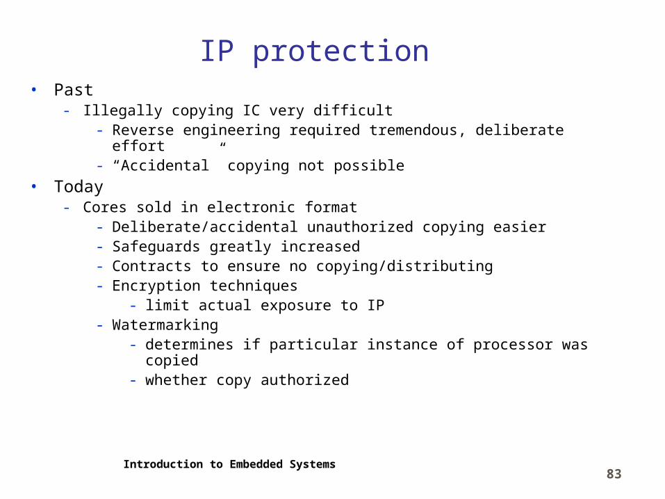
IP protection• Past

- Illegally copying IC very difficult- Reverse engineering required tremendous, deliberate effort- “Accidental” copying not possible

• Today- Cores sold in electronic format

- Deliberate/accidental unauthorized copying easier- Safeguards greatly increased- Contracts to ensure no copying/distributing- Encryption techniques

- limit actual exposure to IP- Watermarking

- determines if particular instance of processor was copied- whether copy authorized


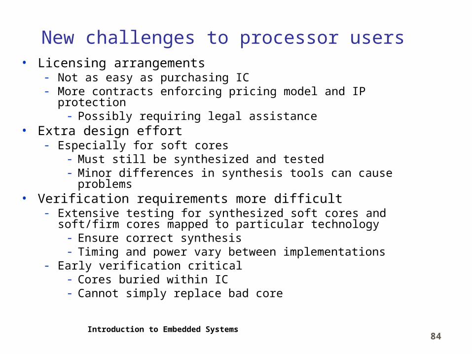
New challenges to processor users• Licensing arrangements

- Not as easy as purchasing IC- More contracts enforcing pricing model and IP protection

- Possibly requiring legal assistance• Extra design effort

- Especially for soft cores- Must still be synthesized and tested- Minor differences in synthesis tools can cause problems

• Verification requirements more difficult- Extensive testing for synthesized soft cores and soft/firm cores

mapped to particular technology- Ensure correct synthesis- Timing and power vary between implementations

- Early verification critical- Cores buried within IC- Cannot simply replace bad core


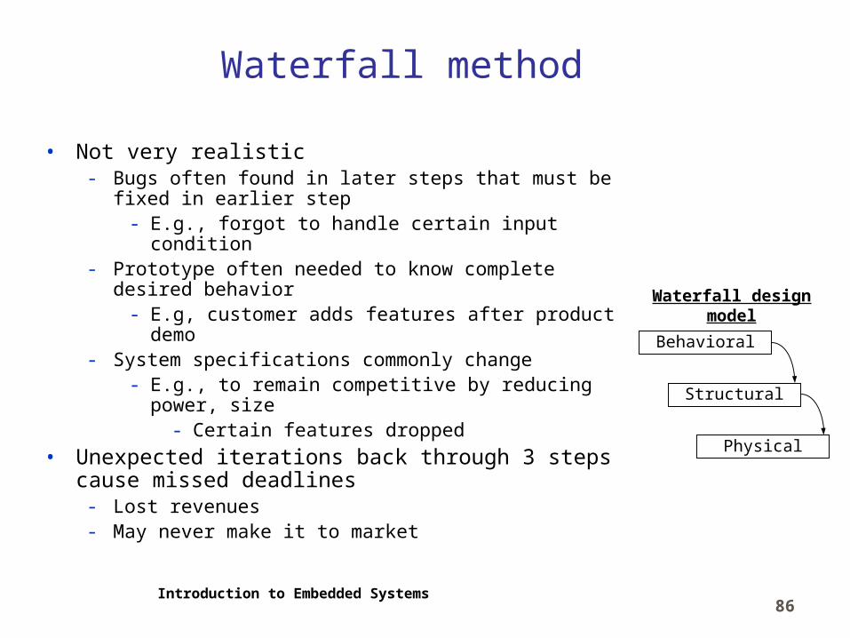
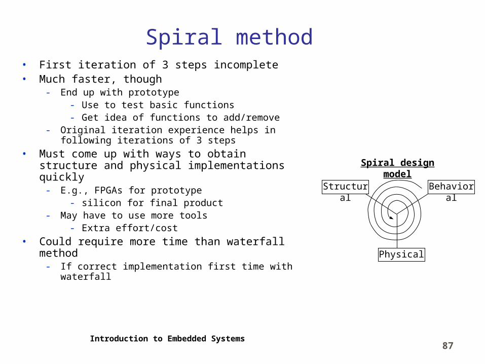
Design process model

• Describes order that design steps are processed

- Behavior description step- Behavior to structure conversion step- Mapping structure to physical implementation

step• Waterfall model

- Proceed to next step only after current step completed

• Spiral model- Proceed through 3 steps in order but with less

detail- Repeat 3 steps gradually increasing detail- Keep repeating until desired system obtained- Becoming extremely popular (hardware &

software development)

Behavioral

Structural

Physical

Waterfall design model

BehavioralStructural

Physical

Spiral design model


Waterfall method

• Not very realistic- Bugs often found in later steps that must be fixed in

earlier step- E.g., forgot to handle certain input condition

- Prototype often needed to know complete desired behavior

- E.g, customer adds features after product demo- System specifications commonly change

- E.g., to remain competitive by reducing power, size

- Certain features dropped• Unexpected iterations back through 3 steps cause

missed deadlines- Lost revenues- May never make it to market

Behavioral

Structural

Physical

Waterfall design model


Spiral method• First iteration of 3 steps incomplete• Much faster, though

- End up with prototype- Use to test basic functions- Get idea of functions to add/remove

- Original iteration experience helps in following iterations of 3 steps

• Must come up with ways to obtain structure and physical implementations quickly

- E.g., FPGAs for prototype - silicon for final product

- May have to use more tools- Extra effort/cost

• Could require more time than waterfall method- If correct implementation first time with waterfall

BehavioralStructural

Physical

Spiral design model


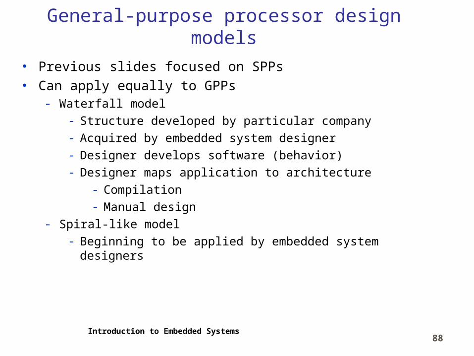
General-purpose processor design models• Previous slides focused on SPPs• Can apply equally to GPPs

- Waterfall model- Structure developed by particular company- Acquired by embedded system designer- Designer develops software (behavior)- Designer maps application to architecture

- Compilation- Manual design

- Spiral-like model- Beginning to be applied by embedded system designers


Spiral-like model

• Designer develops or acquires architecture• Develops application(s)• Maps application to architecture• Analyzes design metrics• Now makes choice

- Modify mapping- Modify application(s) to better suit architecture- Modify architecture to better suit application(s)

- Not as difficult now- Maturation of synthesis/compilers- IPs can be tuned

• Continue refining to lower abstraction level until particular implementation chosen

Architecture Application(s)

Mapping

Analysis

Y-chart

1 the partitioning decision. introduction to embedded systems 2 partitioning hw and sw recall the...

Documents

embedded systemsintroduction

embedded systemassume

software design tools

hardwarethe hardware

software componentscritical

duality of software

costdedicated hardware

total cost