1

The economics of consumption

2

From: President Ella EliTo: Yale StudentsRe: Generous Gift

My dear students,I am delighted to report that a generous alumna has made a

gift of $1000 per Yale student, available immediately. You can come by the office and pick up your check any time.

Professor Nordhaus has requested that you detail how you would spend the funds. Would you please write this down in your notebooks in class today. You will find it instructive as you discuss Consumption in class this week.

With best wishes,President Ella Eli

P.S. Professor Nordhaus has told me about “elevator quizzes,” which are a great idea. This is not an elevator quiz, but you should hold on to your answers for later reference. EE

Importance of consumption in macro1. Consumption is two-thirds of GDP –

understanding its determinants is major part of the ball game.

2. Consumption is the entire point of the economy:

3. Consumption plays two roles in microeconomics:a. AD: It is a major part of AD in the short run: recall IS curve in which Y = C(Yd) + I + G + NXb. AS: What is not consumed is saved and influences national investment and economic growth

3

4

Personal income 12,947 Compensation of employees, received 8,295 64% Proprietors' income 1,157 9% Rental income of persons 410 3% Personal income receipts on assets 1,685 13% Personal current transfer receipts 2,319 18% Less: Contributions for government social insurance, domestic 919Less: Personal current taxes 1,398Equals: Disposable personal income 11,549Less: Personal outlays 11,060Equals: Personal saving 489 Personal saving as a percentage of disposable personal income 4.2

Table 2.1. Personal Income and Its Disposition[Billions of dollars]Bureau of Economic AnalysisLast Revised on: August 29, 2012

Item 2011 Percent of income

5

Personal consumption expenditures 10,729 Goods 3,625 33.8% Durable goods 1,146 10.7% Motor vehicles and parts 374 3.5% Furnishings and durable household equipment 252 2.3% Recreational goods and vehicles 340 3.2% Other durable goods 181 1.7% Nondurable goods 2,478 23.1% Food and beverages purchased, off-premises 810 7.6% Clothing and footwear 349 3.3% Gasoline and other energy goods 428 4.0% Other nondurable goods 891 8.3%Services 7,104 66.2% Housing and utilities 1,930 18.0% Health care 1,752 16.3% Transportation services 302 2.8% Recreation services 395 3.7% Food services and accommodations 671 6.3% Financial services and insurance 807 7.5% Other services 956 8.9% Higher education 168 1.6%

by Type of ProductTable 2.4.5. Personal Consumption Expenditures

[Billions of dollars]Bureau of Economic AnalysisLast Revised on: August 02, 2012

  2011

Growth in C and GDP (quarterly)

6

-.03

-.02

-.01

.00

.01

.02

00 01 02 03 04 05 06 07 08 09 10 11

ConsumptionGDP

Chicken or egg: - ΔC causes

recession?- Recession causes

ΔC?

7

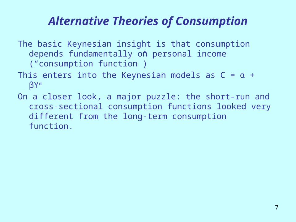
Alternative Theories of Consumption

The basic Keynesian insight is that consumption depends fundamentally on personal income (“consumption function”)

This enters into the Keynesian models as C = α + βYd

On a closer look, a major puzzle: the short-run and cross-sectional consumption functions looked very different from the long-term consumption function.

Consumption and Disposable Income

8

0

2,000

4,000

6,000

8,000

10,000

12,000

0 2,000 4,000 6,000 8,000 10,000 12,000

Real disposable income

Rea

l co

nsu

mp

tion

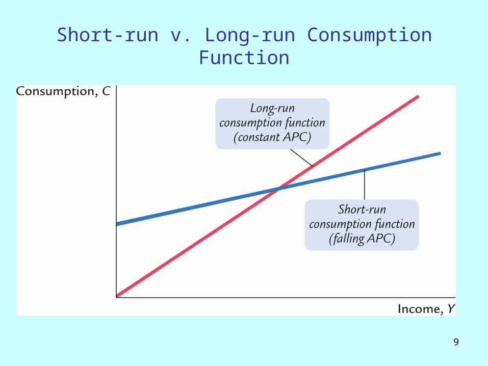
Short-run v. Long-run Consumption Function

9

10

Alternative Theories of Consumption

There are four major approaches in macroeconomics:*1. Fisher's approach: sometimes called the neoclassical

model 2. Keynes original approach of the consumption function*3. Life-cycle or permanent income approaches (Modigliani,

Friedman) 4.Rational expectations (Euler equation) approaches (in

Jones)

*We will do in class, but more Fisher in section.

11

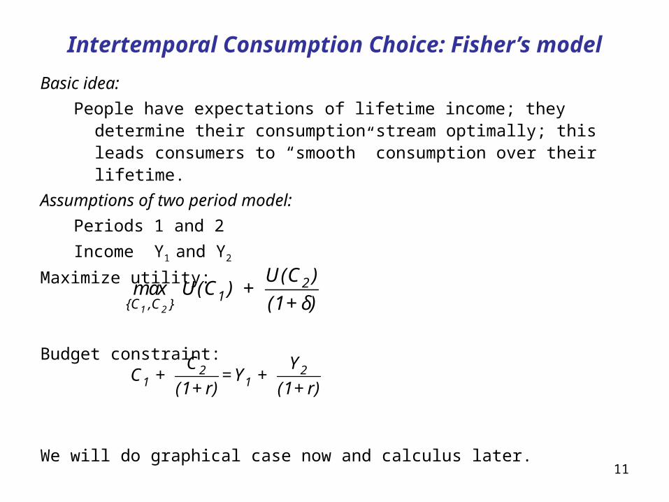
Intertemporal Consumption Choice: Fisher’s model

Basic idea:

People have expectations of lifetime income; they determine their consumption stream optimally; this leads consumers to “smooth” consumption over their lifetime.

Assumptions of two period model:

Periods 1 and 2

Income Y1 and Y2

Maximize utility:

Budget constraint:

We will do graphical case now and calculus later.

2 21 1

C YC + = Y +

(1+r) (1+r)

1 2

21{C ,C }

U(C )max U(C ) +

(1+δ)

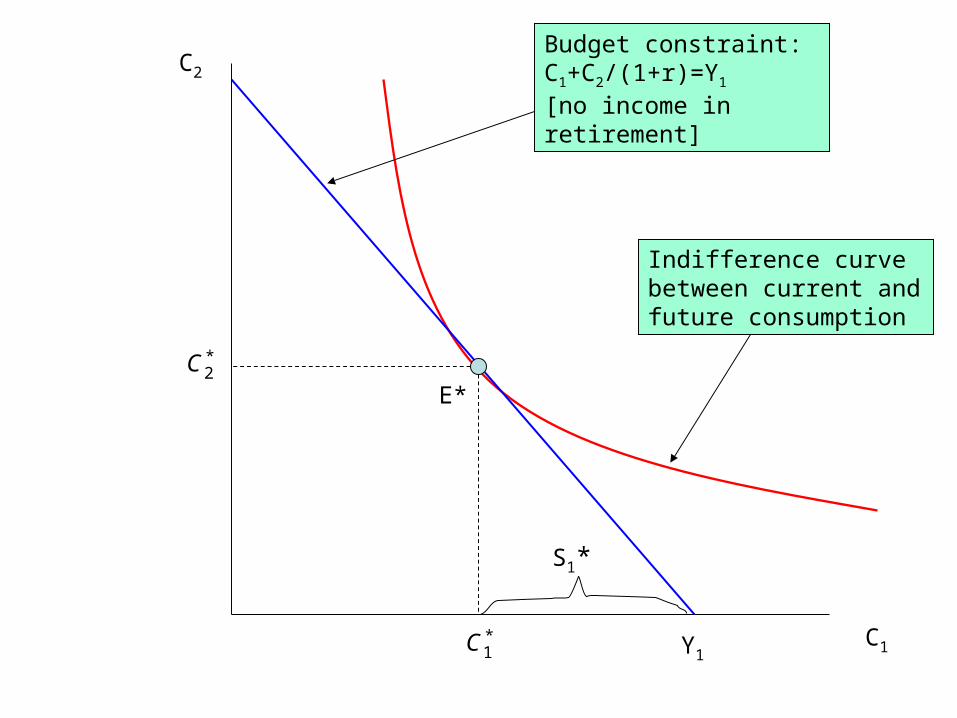
C1

C2

Budget constraint:C1+C2/(1+r)=Y1

[no income in retirement]

Y1

Indifference curve between current and future consumption

E*

S1*

*1C

*2C

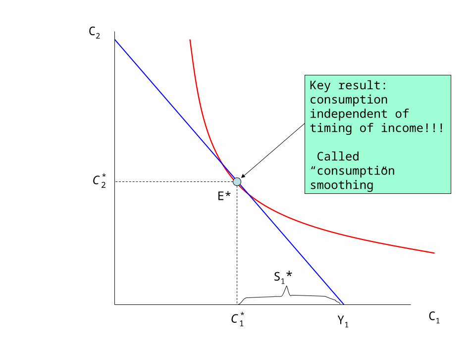
C1

C2

Key result: consumption independent of timing of income!!!

Called “consumption smoothing”

Y1

E*

S1*

*1C

*2C

Summary to hereIncome over life cycle is the major determinant of

consumption and saving.In idealized case, have consumption smoothing over

lifetime.Now move from two-period (Fisher model) to multi-

period (life cycle model).

14

15

Basic Assumptions of Life Cycle Model

Basic idea:People have expectations of lifetime income; they determine

their consumption stream optimally; this leads consumers to “smooth” consumption over their lifetime.

Assumptions:“Life cycle” for planning from age 1 to D.Earn Y per year for ages 1 to R.Retire from R to D.Maximize utility function:

Budget constraint:

Discount rate on utility (δ) = real interest rate (r) = 0 (for simplicity)

D D-z -z

z zz 1 z 1

(1 ) C (1 ) Y r r

1 21

max (1 ) ( ), for ages z 1 to D.D

zD z

z

V(C , C , ..., C ) U C

16

Techniques for Finding Solution

1. Two periods:

Maximizing this leads to U’(C1)=U’(C2). This implies that C1 = C2 , which is consumption smoothing. The Cs are independent of the Ys.

2. Lagrangean maximization (advanced math econ):

Maximizing implies that U’(C1)=U’(C2)=-λ. This implies that

which again is consumption smoothing independent of Y.

z

D D D-z -z -z

1 D z z z{C } z = 1 z = 1 z = 1

max L C ,...,C = (1+δ) U(C ) + λ (1+r) C - (1+r) Y

1 2 1 1 2 1maxz{C }

U(C ) U(C ) U(C ) U(Y Y - C )

tC C

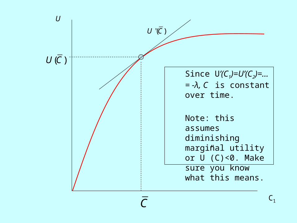
C1

U

C

( )U C

'( )U C

Since U’(C1)=U’(C2)=… = -λ, C is constant over time.

Note: this assumes diminishing marginal utility or U”(C)<0. Make sure you know what this means.

18

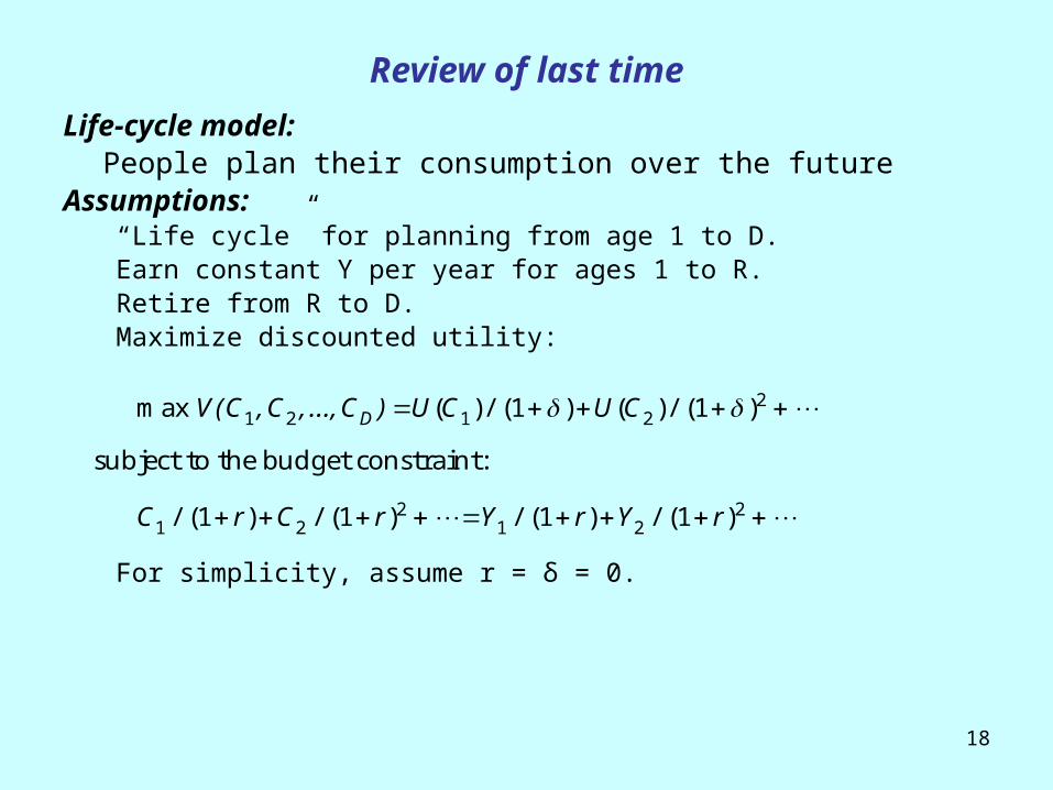
Review of last time

Life-cycle model: People plan their consumption over the future

Assumptions:“Life cycle” for planning from age 1 to D.Earn constant Y per year for ages 1 to R.Retire from R to D.Maximize discounted utility:

For simplicity, assume r = δ = 0.

21 2 1 2

2 21 2 1 2

max ( )/ (1 ) ( )/ (1 )

subject to the budget constraint:

/ (1 ) / (1 ) / (1 ) / (1 )

DV(C , C , ..., C ) U C U C

C r C r Y r Y r

19

age

C, Y, S

Income, Y

R D| |

Consumption, C

0

Saving, S

Diagram of Life Cycle Model Showing Consumption Smoothing

Initial Solution

20

age

C, Y, S

Income, Y

R D| |

Consumption, C’=C

0

Saving, S’

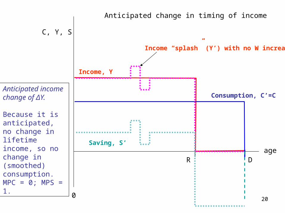
Anticipated change in timing of income

Income “splash” (Y’) with no W increase

Anticipated income change of ΔY.

Because it is anticipated, no change in lifetime income, so no change in (smoothed) consumption. MPC = 0; MPS = 1.

21

age

C, Y, S

Income, Y

R D| |

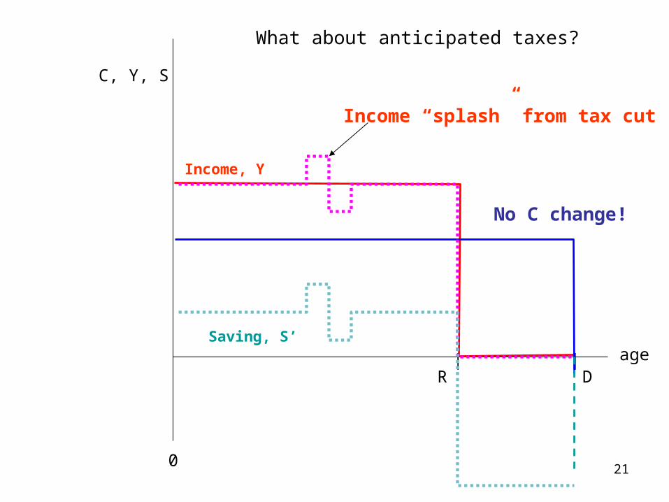
No C change!

0

Saving, S’

What about anticipated taxes?

Income “splash” from tax cut

22

age

C, Y, S

Y

R D| |

C

0

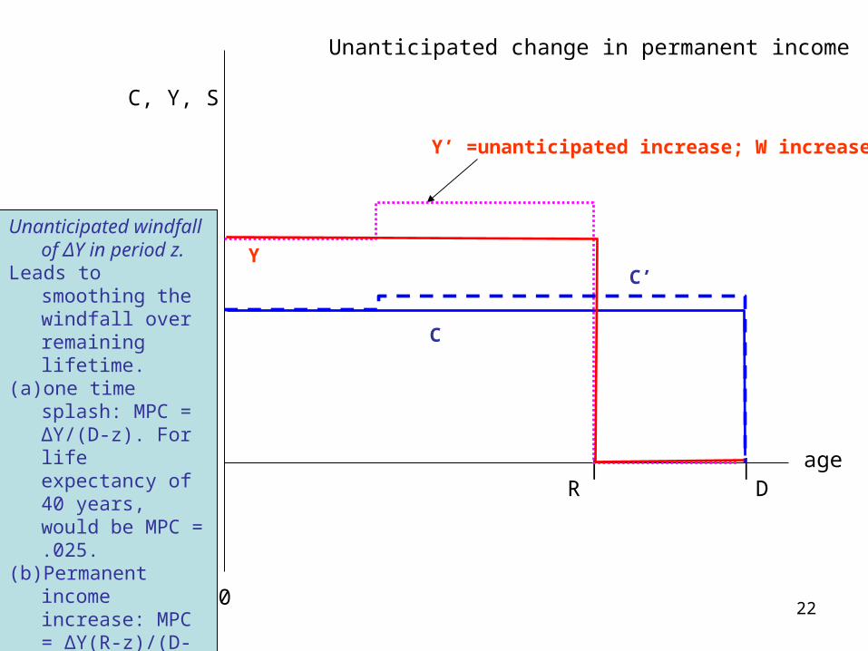
Unanticipated change in permanent income

Y’ =unanticipated increase; W increases.

C’

Unanticipated windfall of ΔY in period z.

Leads to smoothing the windfall over remaining lifetime.

(a) one time splash: MPC = ΔY/(D-z). For life expectancy of 40 years, would be MPC = .025.

(b) Permanent income increase: MPC = ΔY(R-z)/(D-z) = .6 to .8

23

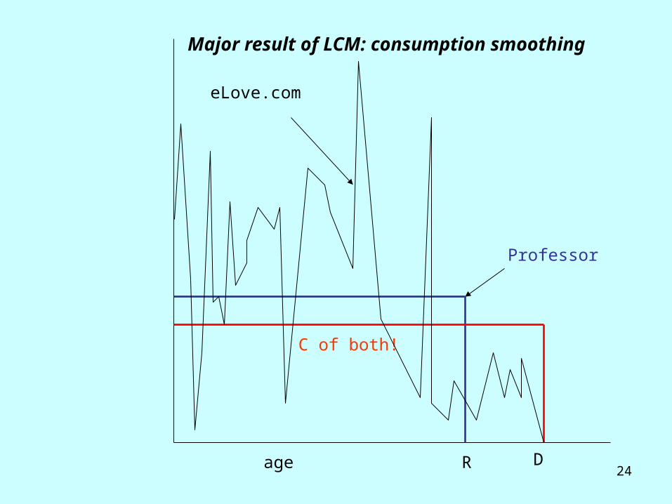
Example of the Life Cycle Model at Work:

• How would the consumption and saving of people with volatile or stable income streams look?

• See figure for Internet Entrepreneur and Yale Professor.

24age

Major result of LCM: consumption smoothing

Professor

C of both!

R D

eLove.com

25

Example of consumption smoothing: the 2008 tax rebate

-400

-200

0

200

400

600

800

06M01 06M07 07M01 07M07 08M01 08M07

CDYS

Changes in C, DY, and S

Estimated MPC= 0.25 (+0.04)

Vector auto-regressions (VAR)Nobel prize in Economics for 2011 won by Chris Sims

(Princeton) in part for development of VAR technique.

Vector autoregression (VAR) is a statistical model used to capture the linear interdependencies among multiple time

series (vector Yt ):

Yt = A0 + A1Yt-1 + A2Yt-2 + A2Yt-2 + et

Sims emphasized it as “theory-free estimation.”

Example of short run MPC using VAR:

MPC = 0.16 ( + 0.04)

Smaller than other estimates because of autoregressive properties.

Summary: Econometric estimates of short-run MPC > life-cycle theory. 26

27

How about a nice car?• What is your favorite car?

• What do you have?

• Why not smooth consumption to get your favorite car?

Liquidity constraints• Case of Yale students where income

growing rapidly.

• Here consumption is limited by borrowing constraint.

• In class: A picture of the model with liquidity constraints.

• Is this reason for MPC higher than life cycle prediction? (Partially, but cannot explain response of non-constrained consumers)

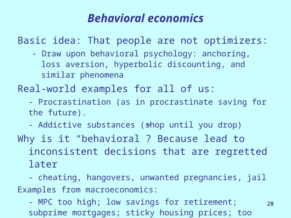
Behavioral economics

Basic idea: That people are not optimizers:- Draw upon behavioral psychology: anchoring, loss

aversion, hyperbolic discounting, and similar phenomena

Real-world examples for all of us: - Procrastination (as in procrastinate saving for the future).

- Addictive substances (shop until you drop)

Why is it “behavioral”? Because lead to inconsistent decisions that are regretted later - cheating, hangovers, unwanted pregnancies, jail

Examples from macroeconomics:

- MPC too high; low savings for retirement; subprime mortgages; sticky housing prices; too high discount rate in energy use 28

29

Press buttonfor Econ 122

Elevator quiz

1. Look back to your answer from Monday on how you would allocate your $1000 unexpected generous gift.

2. Explain how this decision fits into the economics of consumption that we discussed in class and in the textbook.

3. We will discuss our answers when you are done.4. Then hand it in at the end of class.

30

Taxes, interest rates, and saving

“Raise the tax on the returns for saving, and people will save less. We can argue the magnitude, but to argue that saving does not respond at all is simply to argue that incentives and disincentives are irrelevant to behavior.”

“Of Course Higher Taxes Slow Growth,” J.D. Foster and Curtis Dubay

31

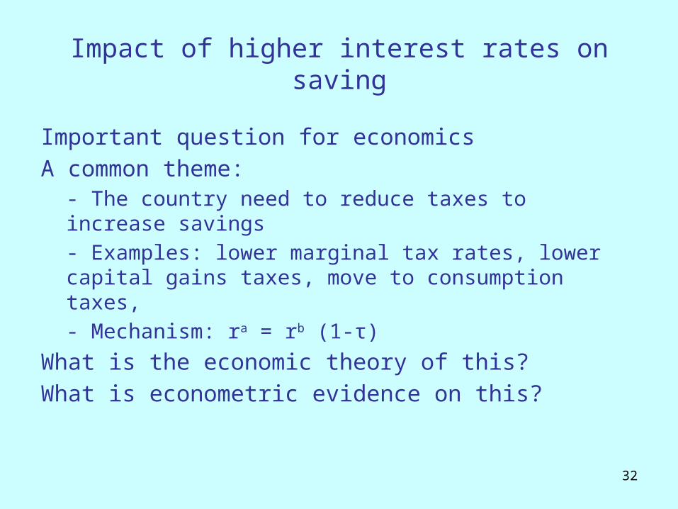
Impact of higher interest rates on saving

Important question for economicsA common theme:

- The country need to reduce taxes to increase savings- Examples: lower marginal tax rates, lower capital gains taxes, move to consumption taxes,

- Mechanism: ra = rb (1-τ)

What is the economic theory of this?What is econometric evidence on this?

32

C1

C2

Y1

E*

E**

CASE I:Higher interest rate leads to lower saving because income effect outweighs substitution effect.

[Pension example]

*1C **

1C

*2C

C1

C2

E*

E**

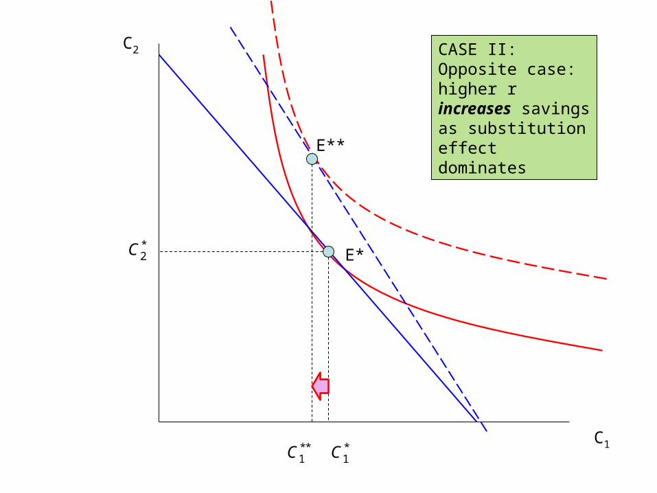
CASE II:Opposite case: higher r increases savings as substitution effect dominates

**1C *

1C

*2C

35

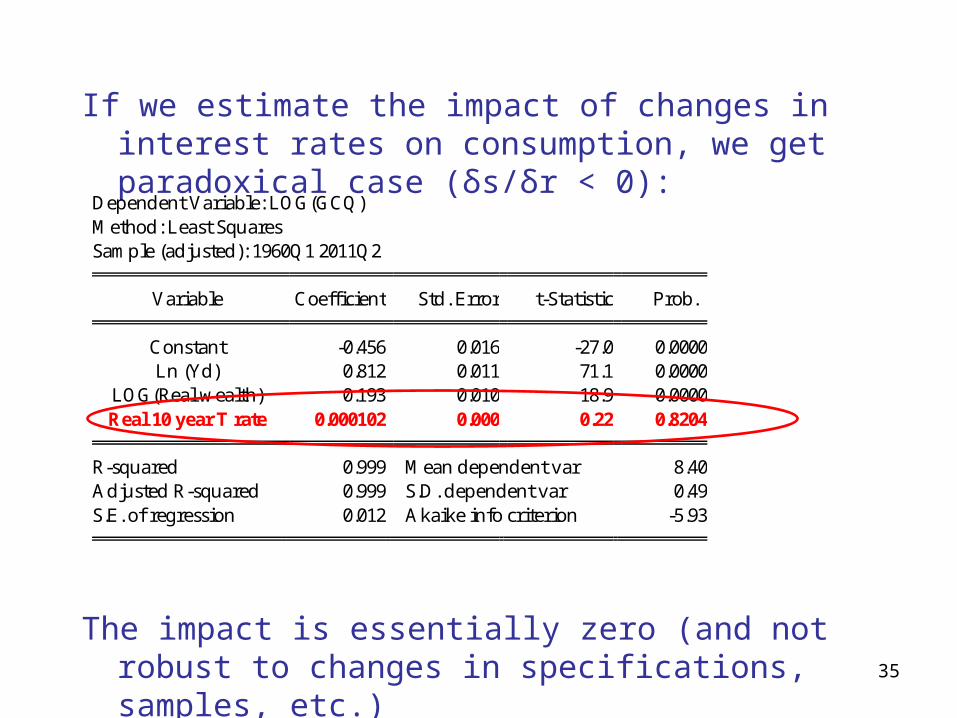
If we estimate the impact of changes in interest rates on consumption, we get paradoxical case (δs/δr < 0):

The impact is essentially zero (and not robust to changes in specifications, samples, etc.)

Dependent Variable: LOG(GCQ) Method: Least Squares Sample (adjusted): 1960Q1 2011Q2

Variable Coefficient Std. Error t-Statistic Prob. Constant -0.456 0.016 -27.0 0.0000

Ln (Yd) 0.812 0.011 71.1 0.0000 LOG(Real wealth) 0.193 0.010 18.9 0.0000 Real 10 year T rate 0.000102 0.000 0.22 0.8204

R-squared 0.999 Mean dependent var 8.40

Adjusted R-squared 0.999 S.D. dependent var 0.49 S.E. of regression 0.012 Akaike info criterion -5.93

Econometric savings schedule: S(r)

36

-6

-4

-2

0

2

4

6

8

10

0 2 4 6 8 10 12 14

Savings rate

Re

al i

nte

rest

ra

te

37

38

0

10

20

30

40

50

1890 1900 1910 1920 1930 1940 1950 1960 1970 1980 1990 2000

Price-earnings ratios, US

Roar

ing 2

0s

Road

ing 9

0s

What is the Effect of Stock Market Booms and Busts on Consumption?

And the housing price collapse…

39

300

250

200

150

100

5088 90 92 94 96 98 00 02 04 06 08 10

Las Vegas, Miami

Detroit

Case-Shiller

Long-term housing trends

40

0

50

100

150

200

250

1880 1900 1920 1940 1960 1980 2000 2020

Rea

l pri

ce o

f ho

usin

g (C

ase-

Shi

ller

inde

x)

Year

Home Prices: estimate as of January 2009

Source: Shiller

41

The Wealth Effect on Consumption

Wealth effects:

– Examples: Suppose the alumna gives you $1000. Or the housing market collapsed as after 2006? What would be the effect on C?

Life cycle model predicts that initial wealth (or surprise inheritances) would be spread over life cycle.

• Intuition: an inheritance is just like an income splash.

So the augmented life cycle model is

Ct = β0 + β1 Yp

t + β2 Wt

where Ypt is permanent or expected

labor income and Wt is wealth.

42

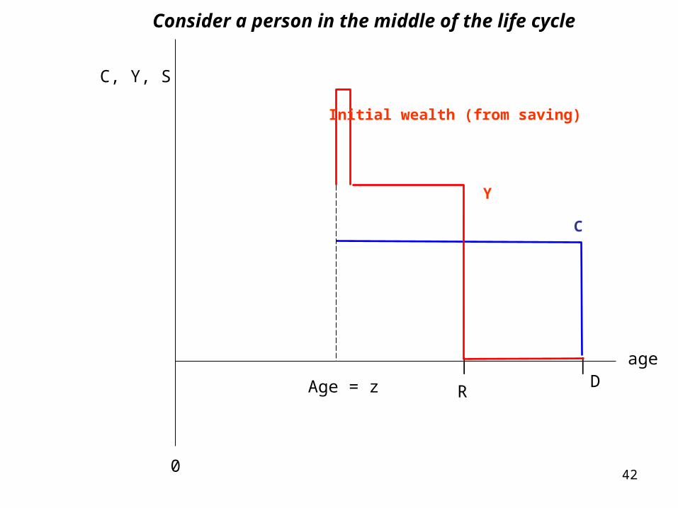
age

C, Y, S

Y

RD

| |

C

0

Initial wealth (from saving)

Age = z

Consider a person in the middle of the life cycle

43

age

C, Y, S

Y

RD

| |

C

0

Wealth shock (falling house prices)

Age = z

Now a wealth shock

C’

44

The stock market, the housing market, and consumption

• Economists think that the bursting of housing bubble was a major source of current recession (US, Spain, ….)

• Reasons? Decline in consumption (today) and investment (later)

• Rationale: the “wealth effect” on consumption• Analysis in the life-cycle model:

– In augmented life-cycle model Ct = β0 +

β1 Yp

t + β2 Wt standard estimates are that β2 = .03 - .06 (example in a minute)

– Effect in the “Roaring 90s” and the housing crash today.

• This is often called “deleveraging” but a better description is a “wealth effect” (leverage is a balance sheet phenomenon).

45

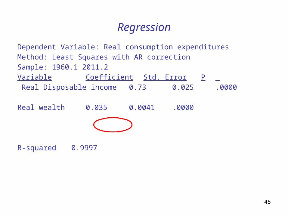
Regression

Dependent Variable: Real consumption expenditures

Method: Least Squares with AR correctionSample: 1960.1 2011.2

Variable Coefficient Std. Error P

Real Disposable income 0.73 0.025 .0000

Real wealth 0.035 0.0041 .0000

R-squared 0.9997

46

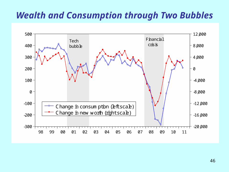
Wealth and Consumption through Two Bubbles

-300

-200

-100

0

100

200

300

400

500

-20,000

-16,000

-12,000

-8,000

-4,000

0

4,000

8,000

12,000

98 99 00 01 02 03 04 05 06 07 08 09 10 11

Change in consumption (left scale)Change in new worth (right scale)

Techbubble

Financial crisis

47

Loss of wealth and savings rate increase

4.4

4.8

5.2

5.6

6.0

6.4

6.8

1

2

3

4

5

6

7

2005 2006 2007 2008 2009 2010 2011

Wea

lth/in

com

eP

ersonal savings rate

Wealth/income (<--) Savings rate (-->)

Key ideas on consumption and saving

1. Consumption derived from consumer maximization

2. Pure model leads to consumption smoothing3. All kinds of important predictions4. But pure model has “anomolies” and shows too

large a short-run MPC relative to theory5. Reasons are probably liquidity constraints and

behavioral frictions.6. Note the impact of interest rates and taxes on

savings.7. Remember the wealth effect

48