1 subject 2 dataset 3 computing the semi-partial correlations - eric

Didacticiel - Études de cas R.R.

1 SubjectComputing semi-partial correlation with Tanagra.

The semi-partial correlation measures the additional information of an independent variable (X),

compared with one or several control variables (Z1,..., Zp), that we can used for the explanation of

a dependent variable (Y).

We can compute the semi-partial correlation in various ways.

The square of the semi-partial correlation can be obtained with the difference between the square

of the multiple correlation coefficient of regression Y / X, Z1...,Zp (including X) and the same

quantity for the regression Y / Z,...,Zp (without X).

We can also obtain the semi-partial correlation by computing the residuals of the regression

X/Z1,...,Zp; then, we compute the correlation between Y and these residuals. In other words, we

seek to quantify the relationship between X and Y, by removing the effect of Z on the latter. The

semi-partial correlation is an asymmetrical measure.

In this tutorial, we show the different ways of producing the semi-partial correlation. We compare

the results with the dedicated tool of TANAGRA (SEMI-PARTIAL CORRELATION).

2 DatasetWe want to explain the consumption of vehicles (Y: CONSUMPTION) from horsepower (X:

HORSEPOWER), by controlling the engine size (Z1: ENGINE.SIZE) and weight (Z2: WEIGHT) effect.

The aim is to determine the additional information of HORESPOWER compared to the control

variables.

3 Computing the semi-partial correlations

3.1 Dataset importation

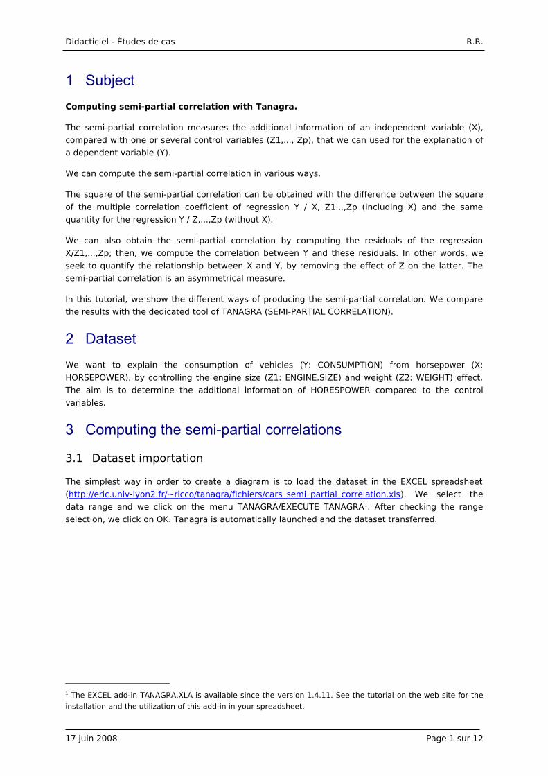
The simplest way in order to create a diagram is to load the dataset in the EXCEL spreadsheet

(http://eric.univ-lyon2.fr/~ricco/tanagra/fichiers/cars_semi_partial_correlation.xls). We select the

data range and we click on the menu TANAGRA/EXECUTE TANAGRA1. After checking the range

selection, we click on OK. Tanagra is automatically launched and the dataset transferred.

1 The EXCEL add-in TANAGRA.XLA is available since the version 1.4.11. See the tutorial on the web site for the

installation and the utilization of this add-in in your spreadsheet.

17 juin 2008 sur 12

http://eric.univ-lyon2.fr/~ricco/tanagra/fichiers/cars_semi_partial_correlation.xls


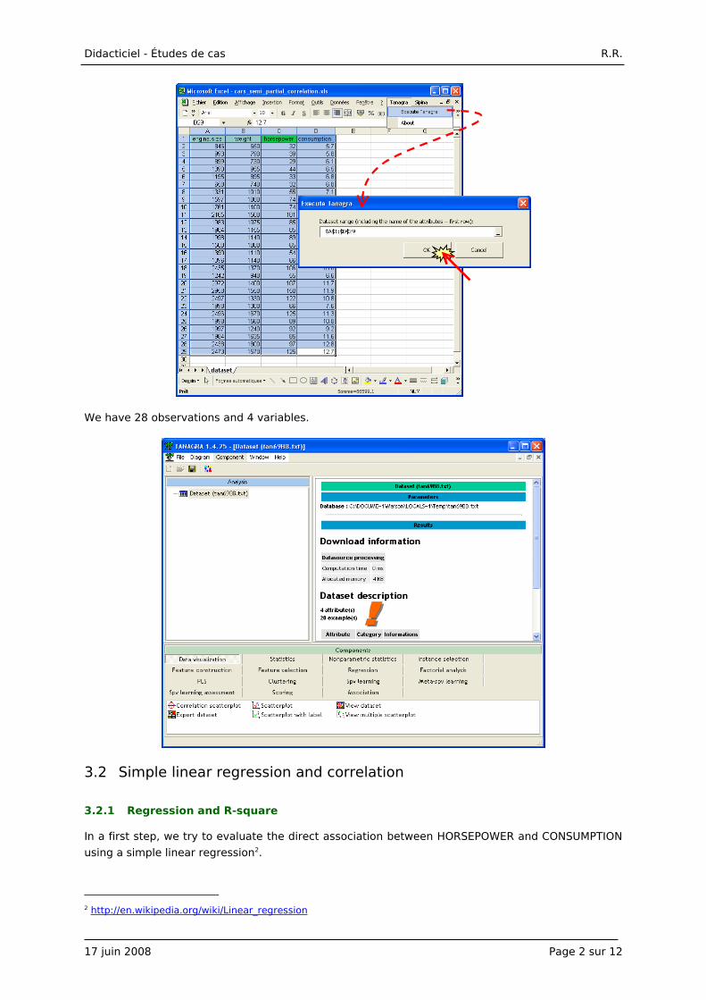
We have 28 observations and 4 variables.

3.2 Simple linear regression and correlation

3.2.1 Regression and R-square

In a first step, we try to evaluate the direct association between HORSEPOWER and CONSUMPTION

using a simple linear regression2.

2 http://en.wikipedia.org/wiki/Linear_regression

17 juin 2008 sur 12

http://en.wikipedia.org/wiki/Linear_regression


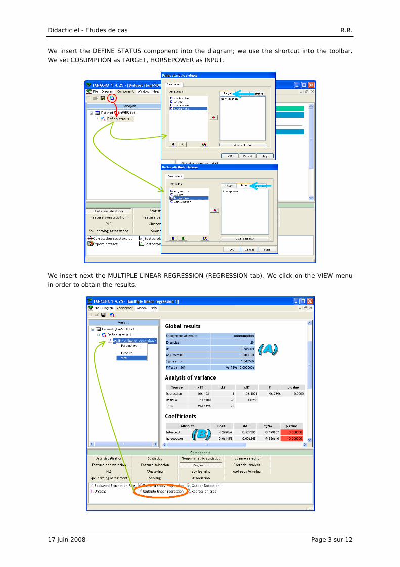
We insert the DEFINE STATUS component into the diagram; we use the shortcut into the toolbar.

We set COSUMPTION as TARGET, HORSEPOWER as INPUT.

We insert next the MULTIPLE LINEAR REGRESSION (REGRESSION tab). We click on the VIEW menu

in order to obtain the results.

17 juin 2008 sur 12


We highlight two main results: (A) the R-square = 0.7882 i.e. 78.82% of the variance of

CONSUMPTION is explained by the regression, it is rather a good result; (B) the HORSEPOWER is

highly significant, the t statistic is 9.8366 with a p-value < 0.0001.

In despite of this encouraging result, we note that there are other variables in our dataset. Perhaps,

they are useful for the explanation of the CONSUMPTION. We analyze deeply this way later (section

3.2.2).

3.2.2 Correlation

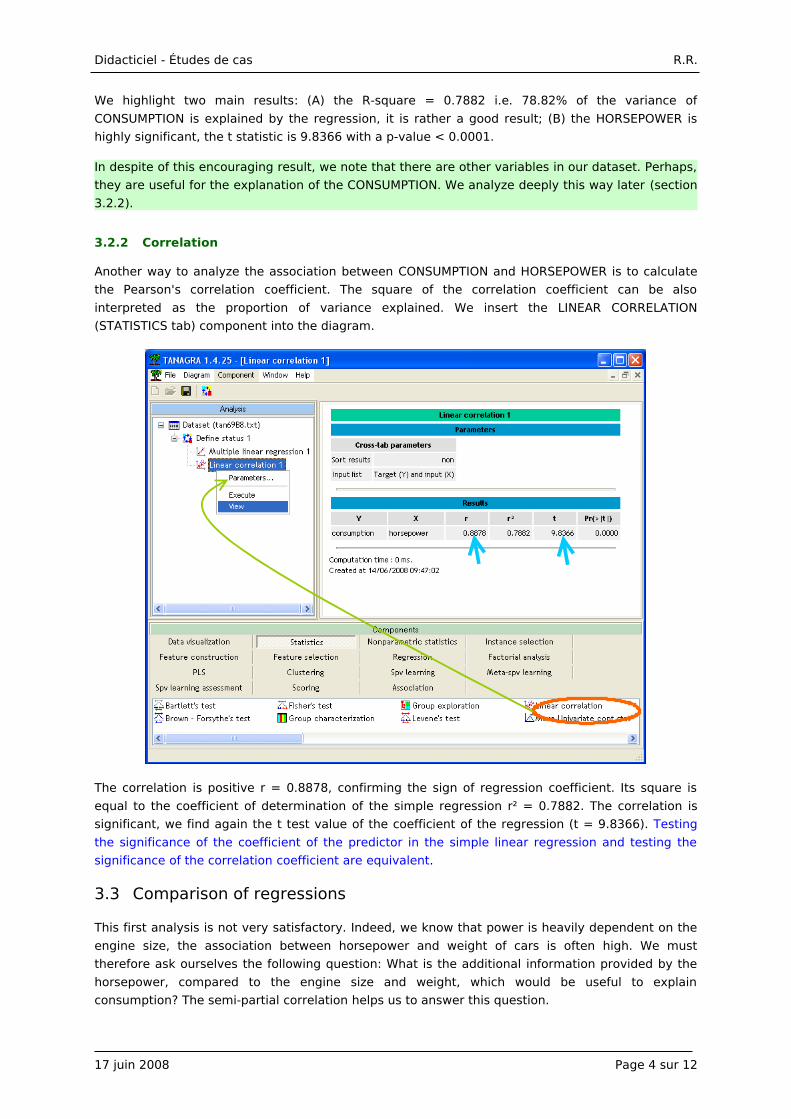
Another way to analyze the association between CONSUMPTION and HORSEPOWER is to calculate

the Pearson's correlation coefficient. The square of the correlation coefficient can be also

interpreted as the proportion of variance explained. We insert the LINEAR CORRELATION

(STATISTICS tab) component into the diagram.

The correlation is positive r = 0.8878, confirming the sign of regression coefficient. Its square is

equal to the coefficient of determination of the simple regression r² = 0.7882. The correlation is

significant, we find again the t test value of the coefficient of the regression (t = 9.8366). Testing

the significance of the coefficient of the predictor in the simple linear regression and testing the

significance of the correlation coefficient are equivalent.

3.3 Comparison of regressions

This first analysis is not very satisfactory. Indeed, we know that power is heavily dependent on the

engine size, the association between horsepower and weight of cars is often high. We must

therefore ask ourselves the following question: What is the additional information provided by the

horsepower, compared to the engine size and weight, which would be useful to explain

consumption? The semi-partial correlation helps us to answer this question.

17 juin 2008 sur 12


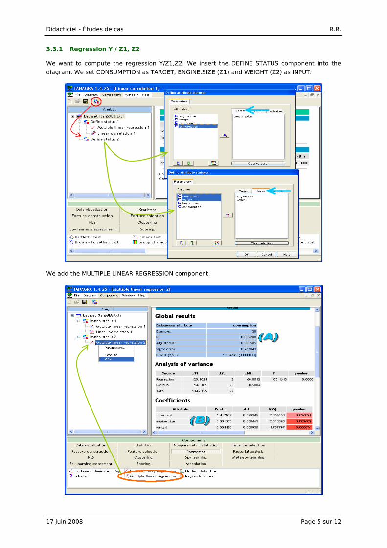
3.3.1 Regression Y / Z1, Z2

We want to compute the regression Y/Z1,Z2. We insert the DEFINE STATUS component into the

diagram. We set CONSUMPTION as TARGET, ENGINE.SIZE (Z1) and WEIGHT (Z2) as INPUT.

We add the MULTIPLE LINEAR REGRESSION component.

17 juin 2008 sur 12


The R-square is high: 89.22% of the variance is explained by the regression (A). All the Z1 and Z2

variables are significant (p-value < 0.01) (B). This regression seems more powerful than the

regression using HORSEPOWER only above (R-square = 0.7882; but the comparison is not really

relevant, we have not the same degrees of freedom).

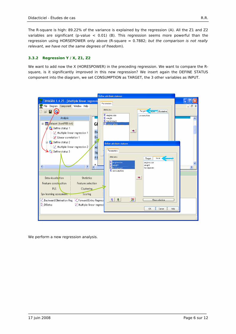
3.3.2 Regression Y / X, Z1, Z2

We want to add now the X (HORESPOWER) in the preceding regression. We want to compare the R-

square, is it significantly improved in this new regression? We insert again the DEFINE STATUS

component into the diagram, we set CONSUMPTION as TARGET, the 3 other variables as INPUT.

We perform a new regression analysis.

17 juin 2008 sur 12


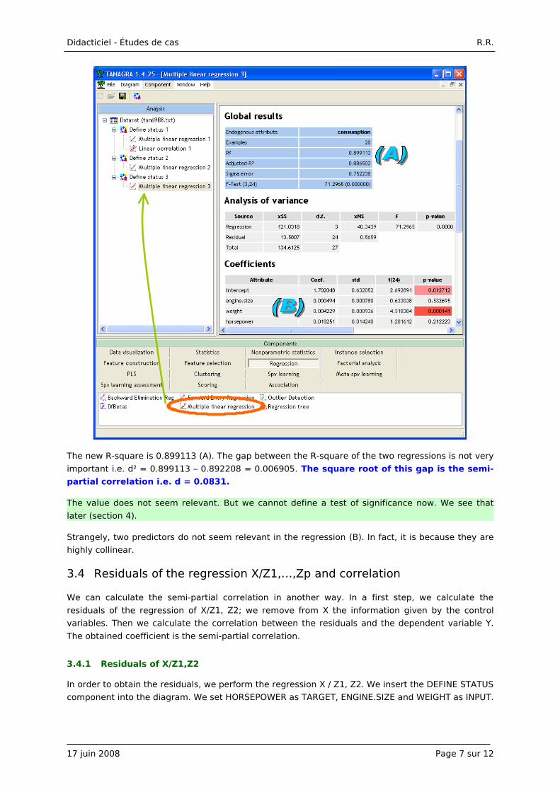
The new R-square is 0.899113 (A). The gap between the R-square of the two regressions is not very

important i.e. d² = 0.899113 – 0.892208 = 0.006905. The square root of this gap is the semi-

partial correlation i.e. d = 0.0831.

The value does not seem relevant. But we cannot define a test of significance now. We see that

later (section 4).

Strangely, two predictors do not seem relevant in the regression (B). In fact, it is because they are

highly collinear.

3.4 Residuals of the regression X/Z1,…,Zp and correlation

We can calculate the semi-partial correlation in another way. In a first step, we calculate the

residuals of the regression of X/Z1, Z2; we remove from X the information given by the control

variables. Then we calculate the correlation between the residuals and the dependent variable Y.

The obtained coefficient is the semi-partial correlation.

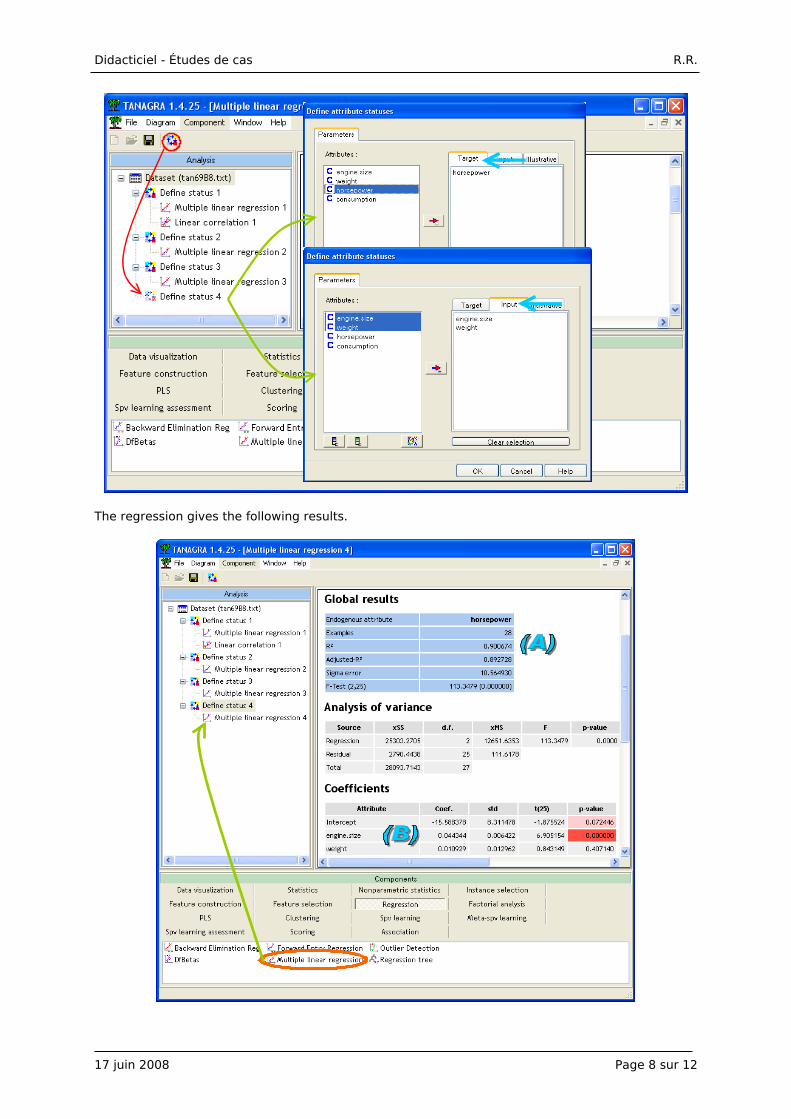
3.4.1 Residuals of X/Z1,Z2

In order to obtain the residuals, we perform the regression X / Z1, Z2. We insert the DEFINE STATUS

component into the diagram. We set HORSEPOWER as TARGET, ENGINE.SIZE and WEIGHT as INPUT.

17 juin 2008 sur 12


The regression gives the following results.

17 juin 2008 sur 12


R² = 90.07% of the variance of HORSEPOWER is explained by the regression (A); essentially by the

predictor ENGINE.SIZE if we consider the p-value of the test of significance (B). Definitely,

HORSEPOWER is highly redundant with the control variables.

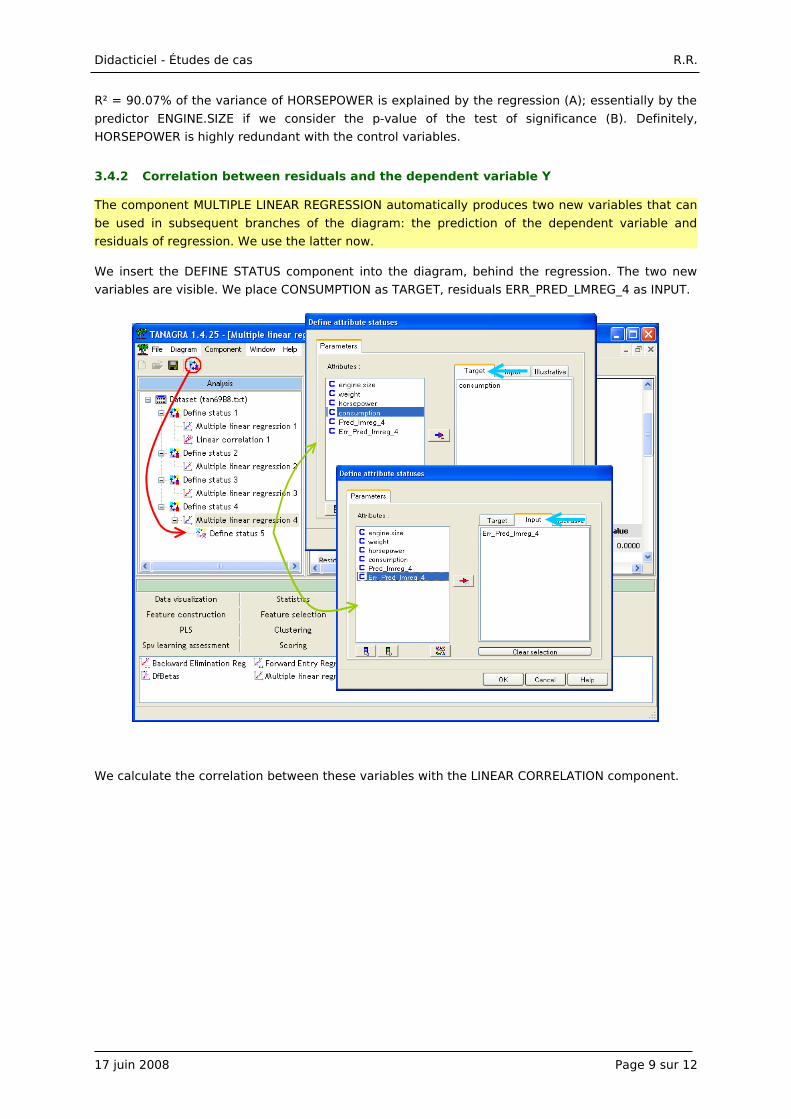
3.4.2 Correlation between residuals and the dependent variable Y

The component MULTIPLE LINEAR REGRESSION automatically produces two new variables that can

be used in subsequent branches of the diagram: the prediction of the dependent variable and

residuals of regression. We use the latter now.

We insert the DEFINE STATUS component into the diagram, behind the regression. The two new

variables are visible. We place CONSUMPTION as TARGET, residuals ERR_PRED_LMREG_4 as INPUT.

We calculate the correlation between these variables with the LINEAR CORRELATION component.

17 juin 2008 sur 12


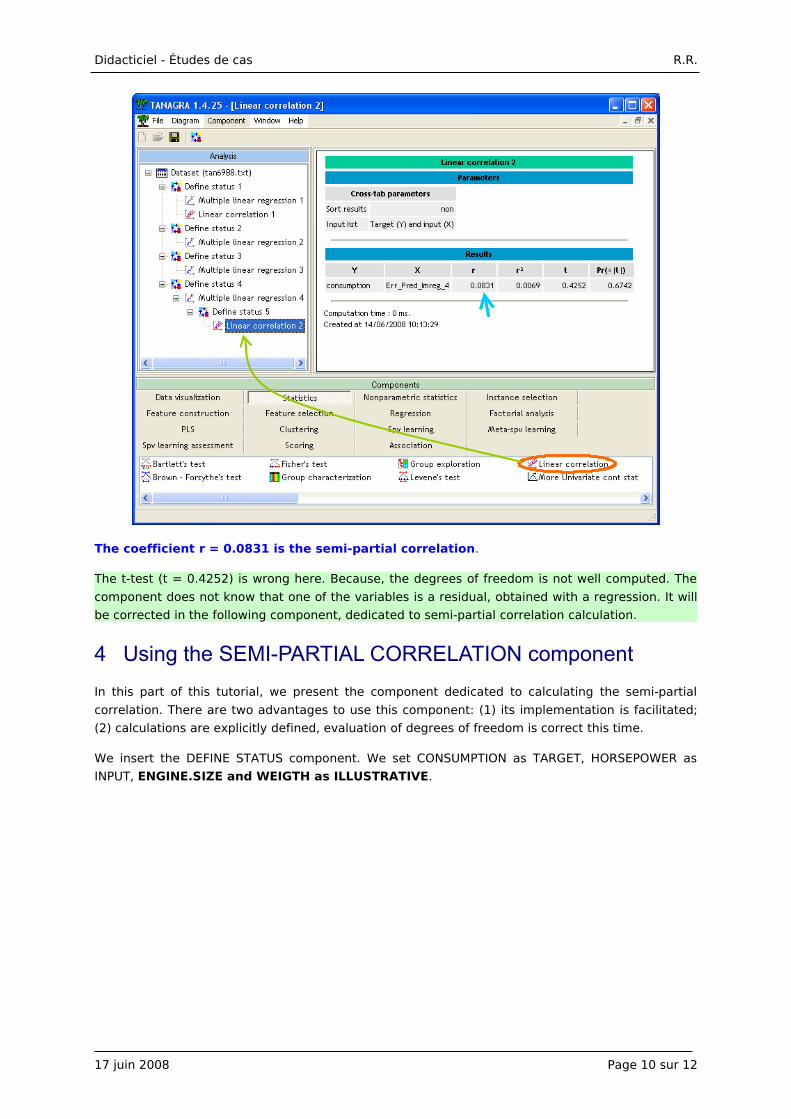
The coefficient r = 0.0831 is the semi-partial correlation.

The t-test (t = 0.4252) is wrong here. Because, the degrees of freedom is not well computed. The

component does not know that one of the variables is a residual, obtained with a regression. It will

be corrected in the following component, dedicated to semi-partial correlation calculation.

4 Using the SEMI-PARTIAL CORRELATION componentIn this part of this tutorial, we present the component dedicated to calculating the semi-partial

correlation. There are two advantages to use this component: (1) its implementation is facilitated;

(2) calculations are explicitly defined, evaluation of degrees of freedom is correct this time.

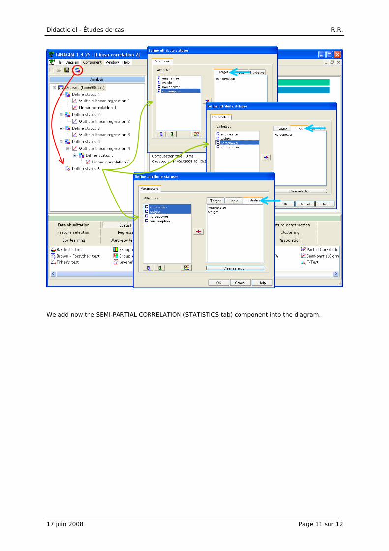
We insert the DEFINE STATUS component. We set CONSUMPTION as TARGET, HORSEPOWER as

INPUT, ENGINE.SIZE and WEIGTH as ILLUSTRATIVE.

17 juin 2008 sur 12


We add now the SEMI-PARTIAL CORRELATION (STATISTICS tab) component into the diagram.

17 juin 2008 sur 12


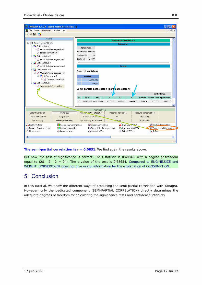
The semi-partial correlation is r = 0.0831. We find again the results above.

But now, the test of significance is correct. The t-statistic is 0.40849, with a degree of freedom

equal to (28 - 2 - 2 = 24). The p-value of the test is 0.68654. Compared to ENGINE.SIZE and

WEIGHT, HORSEPOWER does not give useful information for the explanation of CONSUMPTION.

5 ConclusionIn this tutorial, we show the different ways of producing the semi-partial correlation with Tanagra.

However, only the dedicated component (SEMI-PARTIAL CORRELATION) directly determines the

adequate degrees of freedom for calculating the significance tests and confidence intervals.

17 juin 2008 sur 12

1 subject 2 dataset 3 computing the semi-partial correlations - eric

Documents