energies

Article

Analyzing Oil Price Shocks and Exchange RatesMovements in Korea using MarkovRegime-Switching Models

Suyi Kim 1,† , So-Yeun Kim 1,† and Kyungmee Choi 2,*1 College of Business Management, Hongik University, Sejong-si 30016, Korea; suyikim@hongik.ac.kr (S.K.);

s22kim@hongik.ac.kr (S.-Y.K.)2 College of Science and Technology, Hongik University, Sejong-si 30016, Korea* Correspondence: kmchoi@hongik.ac.kr; Tel.: +82-44-860-2237† These authors contributed equally to this work.

Received: 15 October 2019; Accepted: 29 November 2019; Published: 1 December 2019

Abstract: Korea imports all of its crude oil, and is the world’s fifth largest oil importing country.We analyze the effects of oil prices, interest rates, consumer price indexes (CPIs), and industrialproduction indexes (IPIs) on the regime shift behavior of the Korean exchange rates against theUSA from January 1991 to March 2019. We use the Markov regime switching model (MRSM) todetect the regime shift behavior of the movements of Korean exchange rates. In order to select theoptimal MRSM, we fit a total of 30 models considering four explanatory variables. The selectedmodel based on Akaike information criteria (AIC) and maximum log likelihood (MLL) includes thelog-differentials of oil prices, the log-differentials of CPIs compared to those of the US, and its ownauto-regressive terms. Based on the selected MRSM model, throughout all markets, we find evidenceto support the existence of two distinct regimes: a stable regime with low-volatility, and an unstableregime with high-volatility. The regime with high-volatility includes the Asian financial crisis of 1997and the global financial crisis of 2008–2009 in the Korean exchange rates market. In the regime withlow-volatility, the Korean exchange rates are not significantly influenced by any of the explanatoryvariables, except for its own auto-regressive terms. In the regime with high-volatility, the Koreanexchange rates are significantly influenced by the CPIs and oil prices. The transition probabilityfrom the regime with low-volatility to the regime with high-volatility is about ten times that of theopposite case.

Keywords: oil prices; exchange rate; Markov regime switching model

1. Introduction

Oil prices have fluctuated over the last 30 years. Oil prices per barrel have risen to over $140 anddropped to below $20. Although energy dependence on oil has declined in the past, oil is still one ofthe most important sources of energy. Thus, rising oil prices have a huge impact on the economies ofcountries, which is especially true in those countries that mostly export or import oil. The greater theenergy dependence on oil, the greater the impact oil has on the economy. In particular, Korea importsall of its oil and is the one of the world’s top 10 oil importers. As a result, oil price fluctuations have alarge impact on the trade balance and also on the supply and demand of dollars in the foreign exchangemarket. This seems to have further led to fluctuations in exchange rates. Thus, analyzing how oil pricesaffect the exchange rates has been one of the major concerns of economists. Previous studies whichhave analyzed the relationship between oil prices and exchange rates are Amano and Van Norden [1],Amano and Van Norden [2], Chaudhuri and Daniel [3], Chen and Chen [4], Lizardo and Mollick [5],

Energies 2019, 12, 4581; doi:10.3390/en12234581 www.mdpi.com/journal/energies

Energies 2019, 12, 4581 2 of 16

Basher et al. [6], Aloui et al. [7], Chen et al. [8], Volkov and Yuhn [9], Chen et al. [10], Basher et al. [11],Yang et al. [12], and so on (see Table 1).

Most of these studies not only analyzed the direct relationship between oil prices and the exchangerates, but also analyzed the relationships with other macroeconomic variables, using the macroeconomicmodel. Most of the analyses focused on developed countries, including the US, and oil-exportingcountries, such as Brazil, Canada, Mexico, Norway, Russia, and the United Kingdom. Basher et al. [11]and Yang et al. [12] included Korea in their analyses; however, there have been no studies that haveanalyzed only Korea in-depth.

The methodologies used by most of the studies vary from the error correction model (ECM),the vector error correction model (VECM), structural vector auto-regression (SVAR), generalizedauto-regressive conditional heteroscedasticity (GARCH), and generalized auto-regressive conditionalheteroscedasticity M (GARCH-M). Recently, methodologies such as the Markov regime switchingmodel (Basher et al., [11]) and wavelet coherence analyses (Yang et al., [12]) have been introduced.The methodologies introduced so far are presented in Table 1.

Table 1. Previous studies on the dynamics of oil prices and exchange rates.

Authors Countries Periods Methods Main Results

Amano andVan Norden [1]

Germany, Japan,USA 1973.01–1993.06 Cointegration, granger

causality, FMOLS

Oil shocks could be the most importantfactor determining real exchange rates

in the long run

Amano andVan Norden [2] USA 1972.02–1993.01 ECM (error correction

model), Granger causalityOil prices may have been the dominant

source of persistent real shocks

Chaudhuri andDaniel [3] 16 OECD countries 1973.01–1996.02 ECM (error correction

model), Granger causality

US dollar real exchange rates are due tothe non-stationarity in the real price

of oil.

Chen and Chen [4] G7 countries 1972.01–2005.10 Panel cointegration,FMOLS, DOLS, and PMG

The real oil prices may have been thedominant source of real exchange

rate movements

Lizardo andMollick [5] USA 1970s–2008 VECM Oil price is significant in the

movements of the exchange rate

Basher et al. [6] Emergingeconomics 1988.01–2008.12 Structural VAR A positive oil price shock leads to an

immediate drop in the exchange rate

Aloui et al. [7]European union,

Canada, UK,Swiss, Japan

2000–2011 copula-GARCH

Evidence of significant and symmetricdependence for almost all the

oil-exchange rate pairs. Increases incrude oil prices were found to coincide

with a depreciation of the dollar

Chen et al. [8] USA 1992.08–2011.12(weekly)

GARCH,CARR,

CARR-MIDAS

Crude oil returns are more negativelyassociated with US dollar returns whenthe US dollar depreciates, as compared

to when it appreciates

Volkov andYuhn [9]

Russia, Brazil,Mexico, Canada,

Norway1998.02–2012.08 GARCH-M,

VECMOil price is significant on exchange rates

in Russia, Brazil, and Mexico

Chen et al. [10] 16 OECD countries 1990.01–2014.12 Structural VAROil price shocks can explain about10–20% of long-term variations in

exchange rates

Basher et al. [11] 9 countries 1 Varies by eachcountry 2 Markov switching model

The significant exchange rateappreciation pressures in oil exporting

economies after oil demand shock

Yang et al. [12] 10 countries 3 1999.01–2014.12 A waveletcoherence analysis

The degree of co-movement betweenthe crude oil price and the exchange

rates deviates over time1 Analysis is conducted for a group of oil exporting countries (Brazil, Canada, Mexico, Norway, Russia, and theUnited Kingdom) and oil importing countries (India, Japan, South Korea). 2 For Canada, Norway, India, Japan,and the United Kingdom, models are estimated over the period February 1976 to February 2014. For the othercountries the estimation period is: Brazil (February 1995 to February 2014), Mexico (December 1993 to February2014), Russia (February 1998 to February 2014), and South Korea (May 1981 to February 2014). 3 Brazil, Canada,Mexico, and Russia are treated as oil-exporting countries, and the EU, India, Japan, and South Korea are treated asoil-importing countries.

Energies 2019, 12, 4581 3 of 16

This study analyzes how oil prices affect the Korean exchange rates in both stable and unstableregimes using the Markov regime switching model (MRSM), taking into account other factorssuch as interest rates, economic growth, and price level. This study differs from previous studiesin several aspects. First, most studies on the relationship between oil prices and exchange ratesexcept Basher et al. [11] have used econometric methodologies such as ECM, VECM, SVAR, GARCH,and GARCH-M. Often a pooled series consists of a few subgroups or regimes with different variancescorresponding to different economic situations. The impact of oil prices on the exchange rates isexpected to vary depending on regimes. Therefore, this study looks for underlying regimes using theMarkov regime switching model (MSRM), fits a separate model in each regime, and then examinesthe effect of oil prices along with major macroeconomic explanatory variables on the exchange rates.Since the regimes are expected to explain many errors, the model in each regime tends to be simple.

Second, not only oil prices but also macroeconomic factors such as price levels, income, and interestrates are the major factors that influence the exchange rates. Except for Volkov and Yuhn [9] andBasher et al. [11], most studies have analyzed only the direct relationship between oil prices andexchange rates. This study analyzes the effects of oil prices on exchange rates in each regime underthe correlation with these macro-economic variables. In addition to discovering regimes, this MRSManalysis tests the significance of oil prices and various macroeconomic variables in each regime.Since regimes stand for different economic situations, the significance of variables also changesdepending on regimes.

Third, this study is limited to Korea. Crude oil is entirely imported in Korea and Korea wasone of the world’s top 10 oil importers. The 10 countries that imported the highest dollar valueworth of crude oil during 2018 are 1. China: US$239.2 billion (20.2% of total crude oil imports),2. United States: $163.1 billion (13.8%), 3. India: $114.5 billion (9.7%), 4. Japan: $80.6 billion (6.8%),5. South Korea: $80.4 billion (6.8%), 6. Netherlands: $48.8 billion (4.1%), 7. Germany: $45.1 billion(3.8%), 8. Spain: $34.2 billion (2.9%), 9. Italy: $32.6 billion (2.8%) and 10. France: $28.5 billion (2.4%)(http://www.worldstopexports.com/crude-oil-imports-by-country/). In 2018, Korea was the world’sfifth largest oil importer. According to Korean Customs Service statistics, crude oil imports in 2018were worth 80,393 million dollars. This amount of imported crude oil accounted for 15% of Korea’stotal imports in 2018. Reflecting this economic situation in Korea, this analysis provides unique resultsfor Korea.

Fourth, this study analyzes the effects of movement of explanatory variables on the movement ofexchange rates, while most of previous studies have analyzed the direct relationship between exchangerates and explanatory macroeconomic variables. Throughout this paper, we use the US data as thebasis for comparison.

Therefore, we use the MRSMs, developed by Hamilton [13]. This methodology is furtherdeveloped into Markov switching auto-regressive conditional heteroscedasticity (MS-ARCH, Cai [14]),Markov switching generalized auto-regressive conditional heteroscedasticity (MS-GARCH, Gray [15]),and Markov switching exponential generalized auto-regressive conditional heteroscedasticity(MS-EGARCH, Henry [16]), among others. The MSRM used in this study was also used in Kim et al. [17]and Kim et al. [18].

We examine the regime shift behavior of exchange rates associated with oil prices, interest rates,consumer price indices, and industrial production indices in the Korean foreign exchange market.For this, we apply the two-regime MRSM (Hamilton, [13]) using monthly data from January 1991 toMarch 2019.

The remainder of this paper is organized as follows. In Section 2, the data and the MSRM areexplained in detail. In Section 3, the model selection is performed and empirical estimation results arepresented based on the selected MRSM, and Section 4 discusses the statistical validity of our modeland assumptions. Finally, the conclusions drawn from this study are presented in Section 5.

Energies 2019, 12, 4581 4 of 16

2. Data and Methods

All monthly data, except for the oil prices, used in this paper are from the OECD (Organizationfor Economic Cooperation and development) data set (OECD.stat) from January 1991 to March 2019.The monthly Korean exchange rates are expressed as the won value needed to purchase one US dollar.The monthly short-run interest rates measured in % are from the monthly monetary and financialstatistics data set of the OECD. The monthly consumer price indices (with the index of 2015 being 100)are from the consumer price indices (CPIs) complete database of the OECD, and the monthly industrialproduction indices (with the index of 2015 being 100) are from the production and sales data set of theOECD. The monthly oil prices which are the CIF (Cost Insurance and Freight) oil importing prices ofAsia measured in US dollars are from KESIS (Korea Energy Statistics Information System) of the KoreaEnergy Economics Institute.

The primary purpose of this study is to analyze how the movement of oil prices affects themovement of the Korean exchange rates in each regime in terms of regime shift behavior. Our researchis based on the monetary model of exchange rates determination which has lead emergence ofthe dominant exchange rates model in early 1970s and henceforward remained as an importantexchange rate paradigm (Frenkel [19], Mussa [20–22], Bilson [23]). Following the monetary model,the exchange rates are determined by the relative supply and demand of money between two givencountries. The money demand is determined by price level, income, interest rates, and other factorsincluding oil prices. Meese and Rogoff [24,25] conducted the seminal work using monetary modelsto forecast exchange rates. They regressed the log of exchange rates on various combinations ofrelative macroeconomic variables which were typically included in the monetary model of exchangerates determination.

Recently, Volkov and Yuhn [9] identified some relevant factors that affect the exchange rates betweenthe United States and the corresponding countries on the basis of the monetary model of exchange ratesdetermination. The fundamental factors include interest rates differentials, income (or production)differentials, and inflation rates differentials between two countries. They excluded the money supplyvariable from the exchange rates determination model to avoid any possible multicollinearity betweenthe money supply and the determining variables of the exchange rates. Since they use monthly data forthe analysis of exchange rates movements, and since monthly GDP figures are not available, industrialproduction is used as a proxy for income.

We consider some relevant variables that affect the exchange rates between Korea and the USAas in Volkov and Yuhn [9]. Oil prices are added to the fundamental factors including interest ratesdifferentials, production differentials, and inflation rates differentials between the two countries.Here, industrial production index (IPI) and consumer price index (CPI) are set as indices representingproduction and inflation, respectively.

The two-regime Markov switching model by Hamilton [1] is an adequate approach to analyze theimpact of these factors (oil prices, interest rates differentials, CPIs differentials, and IPIs differentials)on the movements of Korean exchange rates. In terms of methodology, the auto-regressive terms areconsidered as in the Hamilton models [1]. The MRSM following Hamilton [1] assumes that there aretwo regimes with different volatilities, and that the processes switch between the two regimes accordingto the transition probabilities of the Markov process. Regime 1 consists of low-volatility periods andregime 2 consists of high-volatility periods. Regime 2 is used to identify unstable economic situations.

In this paper, we assume that the logarithms of exchange rates follow a normal distribution asthe logarithms of return rates in equity markets follow a Brownian motion (Osborne, [26]). Often ineconomic data, the log-transformation reinforces the normality assumption and using differentialsreinforces stationarity of the process. At time t, let LEt be the logarithm of the monthly changes inexchange rates compared to the ones from the previous month as follows (Ayodeji [27]):

LEt = log(

Exchange Ratet

Exchange Ratet−1

), (1)

Energies 2019, 12, 4581 5 of 16

LEt lies in one of the two regimes St, where St is 1 or 2. LEt is ∆ log(Exchange Ratet) in theinterval [t− 1, t), which is the change of log(Exchange Ratet). If we consider the time change as∆t = t − (t− 1) = 1, then LEt is the change rate in [t− 1, t). Assuming that the series is an infinitecontinuous process, LEt is an approximate derivative of log(Exchange Ratet) at (t− 1). That is,LEt is the slope of the tangent line to log(Exchange Ratet) which means instantaneous change rate oflog(Exchange Ratet) at (t− 1). Now let us call LEt log-differential of exchange rates. Since regime shiftbehaviors of (Exchange Ratet) and LEt should match, we investigate regimes of exchange rates usingLEt. Note that LEt stands for changes of exchange rates.

Similarly, we transform the four explanatory variables. First, RINTt, RCPIt, and RIPIt are theratios of short-run interest rates, the ratio of consumer price indices and ratio of industrial productionindices between Korea and the USA, respectively. Then, the log-differentials of these ratios ofmacroeconomic variables are obtained as LOILt, LRINTt, LRCPIt, and LRIPIt. The relative differencesof these fundamental variables between the two countries are expected to affect US exchange rates inKorea, as confirmed by Volkov and Yuhn [9]. However, this study regards the variable ratio betweenthe two countries, instead of their direct differences like the study of Volkov and Yuhn [9], because theKorean exchange rates are expressed as ratios with the US dollars as its denominator. The similar formof log-differentials of variables provides the same intrinsic explanation as before.

LOILt = log(

Oil Pricet

Oil Pricet−1

), (2)

LRINTt = log(

RINTt

RINTt−1

), where RINTt =

Interest rate o f Korea at tInterest rate o f USA at t

, (3)

LRCPIt = log(

RCPIt

RCPIt−1

), where RCPIt =

Consumer price index o f Korea at tConsumer price index o f USA at t

, (4)

LRIPIt = log(

RIPIt

RIPIt−1

),where RIPIt =

Industrial production index o f Korea at tIndustrial production index o f USA at t

, (5)

Note that there are two ratios in Equations (3)–(5). First, the ratio between Korea and the USA isevaluated. Secondly, the ratio between time t and time (t− 1) is evaluated. Finally, log-transformationis applied. The LR in front of the variable name stands for log-transformation of the ratio of the ratio.Therefore, we indirectly observe changes in movements of exchange rates through its log-differentials.In each regime, the standard deviation is that of the log-differentials of exchange rates.

The MRSM with the four explanatory variables we consider can be written as follows:

LEt∣∣∣st = β0st + β1st LEt−1 + β2stLOILt + β3st LRINTt + β4st LRCPIt + β5st LRIPIt + εt

∣∣∣st, (6)

where εt|st ∼ N(0, σ2

st

). Our model assumes that the exchange rates switch between the two regimes

based on the Markov transition probabilities which are denoted by

pi j = Pr[st+1 = j∣∣∣st = i], i = 1, 2, j = 1, 2, (7)

where, pi j is the transition probability from state i to state j, pi1 + pi2 = 1, for i = 1, 2. The oil prices, theinterest rates, the CPIs and the IPIs do not switch. We assume that σ2

1 < σ22. The parameter space Θ is

as followsΘ =

β0st , β1st , β2st , β3st , β4st , β5st σ

2st , p12, , p21

, st = 1 or 2. (8)

The filtered probabilities of st are defined as P(st = i∣∣∣Zt; Θ) for i = 1, 2, where Zt stands for all

observations up to time t. In our empirical studies, the process at time t is said to be in regime 1(with low-volatility) if its estimated filtered probability of regime 1 is greater than that of regime 2.Otherwise, the process at time t is said to be in regime 2 (Sanchez-Espigares and Jose [28], Kuan [29]).

Energies 2019, 12, 4581 6 of 16

For model selection, we first fit the full model. Secondly, based on stepwise selection method,we select the most appropriate model using Akaike information criterion (AIC) criterion. Third, theWilks test is performed based on the maximum log-likelihood (MLL) to select the final model based onMaximum Likelihood Estimator (MLE). If the sample size is large, the (−2MLL) difference between thegeneral model and restricted model is asymptotically a chi-squared distribution, with the degrees offreedom as the dimension difference of the two parameter spaces when the restricted model is correct.

The restricted model is assumed under the null hypothesis and the general model is used underthe alternative hypothesis. If MLLr and MLLg are the MLL of the restricted model and the MLL ofthe more general model, respectively, and di is the number of parameters to be estimated in model i,then the difference in MLL asymptotically follows a chi-squared distribution for a large sample:

∆(−2MLL) = (−2MLLr) −(−2MLLg

)→ χ2

(dg − dr

), (9)

If the difference in MLL between any two selected models is significant, then the general model isselected. In addition to the MLL, we use the AIC which considers a penalty to increment of dimensionof the model.

AIC = −2MLL + 2npar (10)

where npar is the number of parameters to be estimated in the model. “The model with smaller AICis better.” (Akaike [30]; Akaike [31]; Pinheiro and Bates, [32]; Rice [33]). The AIC is now one of themost popular model selection criteria in machine learning. Starting from the full model in Equation (6),the variables will be first selected based on AIC, and then significance of each variable in the selectedmodel is tested based on ∆(−2MLL) in Equation (9). We use the msmFit function (Sanchez-Espigaresand Jose, [28]) and the stepAIC function (Venables and Ripley, [34]) in R 3.3.1. Throughout the paper,p-values less than 0.10 are considered to be statistically significant.

3. Results

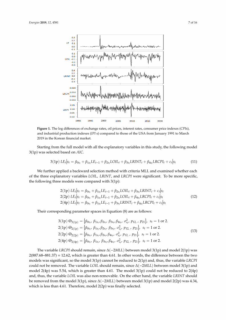
The plots of Figure 1 show time series from January 1991 to March 2019 in the Korean exchangerates market: (1) LE (exchange rates), (2) LOIL (oil prices) (3) LRINT (interest rates between Koreaand the USA.), (4) LRCPI (CPIs between Korea and USA), and (5) LRIPI (IPIs between Korea and theUSA.). Co-movements of high peaks and low valleys are observed in these processes during the Asianfinancial crisis of 1997 and the global financial crisis of 2008–2009.

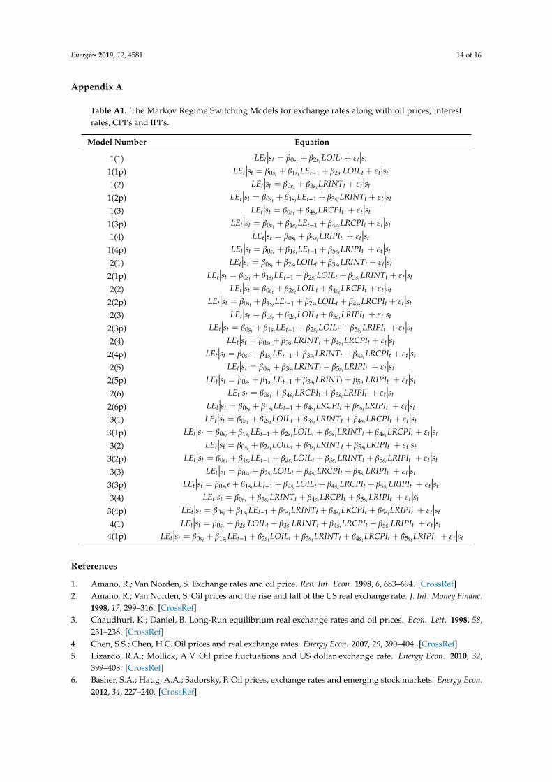
With exchange rates as the response variable, we fit the following thirty two-regime switchingmodels, as shown in Table A1 in Appendix A: (1) eight models with one explanatory variable (from 1 (1)to 1 (4p)); (2) twelve models with two explanatory variables (from 2 (1) to 2 (6p)); (3) eight modelswith three explanatory variables (from 3 (1) to 3 (4p)); and (4) two models with all four explanatoryvariables (from 4 (1) and 4 (1p)). For each model, p stands for the model with the auto-regressive termsof the exchange rates.

We consider the two model selection criteria: MLL and AIC. We first fit the full model inEquation (6). Then, the model with smallest AIC is selected based on the stepwise selection method.In order to reach the final model, significance of each variable in the selected model is further testedone-by-one based on ∆(−2MLL) in Equation (9) and the backward selection method. Note that thedegrees of freedom is 2 since we test one variable at a time which corresponds to the two coefficients,one for the low-volatility period and the other for the high-volatility period. At the significance level0.1, if ∆(−2MLL) > χ2

0.10(2) = 4.61, the variable is said to be significant and remain in the model.Otherwise, it is removed.

For the use of MLL in model selection for MRSM, Hardy [17] mentioned that “even where modelsare not embedded, the likelihood ratio test can be used for model selection, although the χ2 distributionis in this case only an approximation”.

Energies 2019, 12, 4581 7 of 16

Energies 2019, 12, 4581 7 of 16

Figure 1. The log differences of exchange rates, oil prices, interest rates, consumer price indexes (𝐶𝑃𝐼s), and industrial production indexes (𝐼𝑃𝐼s) compared to those of the USA from January 1991 to March 2019 in the Korean financial market.

Starting from the full model with all the explanatory variables in this study, the following model 3(1p) was selected based on 𝐴𝐼𝐶.

3(1p) 𝐿𝐸 |𝑠 = 𝛽 + 𝛽 𝐿𝐸 + 𝛽 𝐿𝑂𝐼𝐿 + 𝛽 𝐿𝑅𝐼𝑁𝑇 + 𝛽 𝐿𝑅𝐶𝑃𝐼 + 𝜀 |𝑠 (11)

We further applied a backward selection method with criteria MLL and examined whether each of the three explanatory variables 𝐿𝑂𝐼𝐿, 𝐿𝑅𝐼𝑁𝑇, and 𝐿𝑅𝐶𝑃𝐼 were significant. To be more specific, the following three models were compared with 3(1p):

2(1p) 𝐿𝐸 |𝑠 = 𝛽 + 𝛽 𝐿𝐸 + 𝛽 𝐿𝑂𝐼𝐿 + 𝛽 𝐿𝑅𝐼𝑁𝑇 + 𝜀 |𝑠

2(2p) 𝐿𝐸 |𝑠 = 𝛽 + 𝛽 𝐿𝐸 + 𝛽 𝐿𝑂𝐼𝐿 + 𝛽 𝐿𝑅𝐶𝑃𝐼 + 𝜀 |𝑠

2(4p) 𝐿𝐸 |𝑠 = 𝛽 + 𝛽 𝐿𝐸 + 𝛽 𝐿𝑅𝐼𝑁𝑇 + 𝛽 𝐿𝑅𝐶𝑃𝐼 + 𝜀 |𝑠

(12)

Their corresponding parameter spaces in Equation (8) are as follows: 3(1p) 𝛩 ( ) = 𝛽 , 𝛽 , 𝛽 , 𝛽 , 𝛽 , 𝜎 , 𝑝 ,, 𝑝 , 𝑠 = 1 or 2.

2(1p) 𝛩 ( ) = 𝛽 , 𝛽 , 𝛽 , 𝛽 , 𝜎 , 𝑝 ,, 𝑝 , 𝑠 = 1 or 2.

2(2p) 𝛩 ( ) = 𝛽 , 𝛽 , 𝛽 , 𝛽 , 𝜎 , 𝑝 ,, 𝑝 , 𝑠 = 1 or 2.

2(4p) 𝛩 ( ) = 𝛽 , 𝛽 , 𝛽 , 𝛽 , 𝜎 , 𝑝 ,, 𝑝 , 𝑠 = 1 or 2.

(13)

The variable 𝐿𝑅𝐶𝑃𝐼 should remain, since ∆(−2𝑀𝐿𝐿) between model 3(1p) and model 2(1p) was 2(887.68-881.37) = 12.62, which is greater than 4.61. In other words, the difference between the two models was significant, so the model 3(1p) cannot be reduced to 2(1p) and, thus, the variable 𝐿𝑅𝐶𝑃𝐼 could not be removed. The variable 𝐿𝑂𝐼𝐿 should remain, since ∆(−2𝑀𝐿𝐿) between model 3(1p) and model 2(4p) was 5.54, which is greater than 4.61. The model 3(1p) could not be reduced to 2(4p) and, thus, the variable 𝐿𝑂𝐼𝐿 was also non-removable. On the other hand, the variable 𝐿𝑅𝐼𝑁𝑇 should be removed from the model 3(1p), since ∆(−2𝑀𝐿𝐿) between model 3(1p) and model 2(2p) was 4.34, which is less than 4.61. Therefore, model 2(2p) was finally selected.

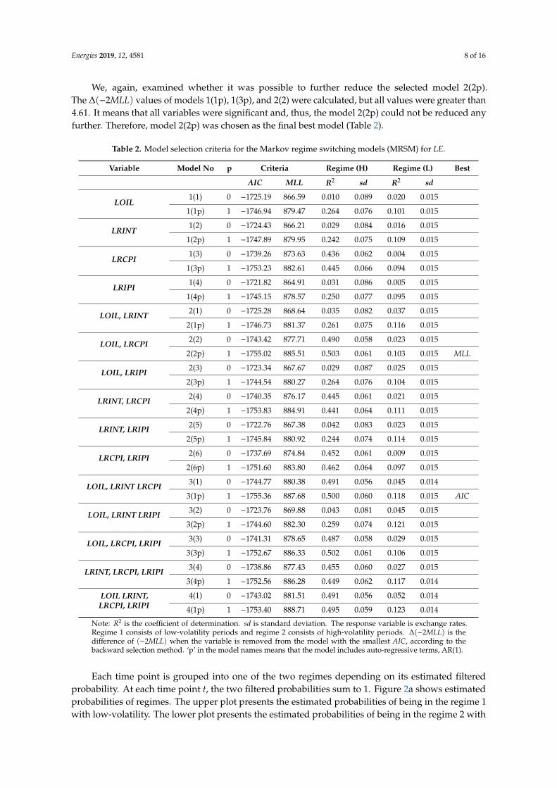
We, again, examined whether it was possible to further reduce the selected model 2(2p). The ∆(−2𝑀𝐿𝐿) values of models 1(1p), 1(3p), and 2(2) were calculated, but all values were greater than 4.61. It means that all variables were significant and, thus, the model 2(2p) could not be reduced any further. Therefore, model 2(2p) was chosen as the final best model (Table 2).

Figure 1. The log differences of exchange rates, oil prices, interest rates, consumer price indexes (CPIs),and industrial production indexes (IPI s) compared to those of the USA from January 1991 to March2019 in the Korean financial market.

Starting from the full model with all the explanatory variables in this study, the following model3(1p) was selected based on AIC.

3(1p) LEt∣∣∣st = β0st + β1st LEt−1 + β2st LOILt + β3st LRINTt + β4stLRCPIt + εt

∣∣∣st (11)

We further applied a backward selection method with criteria MLL and examined whether eachof the three explanatory variables LOIL, LRINT, and LRCPI were significant. To be more specific,the following three models were compared with 3(1p):

2(1p) LEt∣∣∣st = β0st + β1st LEt−1 + β2st LOILt + β3st LRINTt + εt

∣∣∣st

2(2p) LEt∣∣∣st = β0st + β1stLEt−1 + β2st LOILt + β4st LRCPIt + εt

∣∣∣st

2(4p) LEt∣∣∣st = β0st + β1stLEt−1 + β3st LRINTt + β4st LRCPIt + εt

∣∣∣st

(12)

Their corresponding parameter spaces in Equation (8) are as follows:

3(1p) Θ3(1p) =β0st , β1st , β2st , β3st , β4st , σ

2st , p12, , p21

, st = 1 or 2.

2(1p) Θ2(1p) =β0st , β1st , β2st , β3st , σ

2st , p12, , p21

, st = 1 or 2.

2(2p) Θ2(2p) =β0st , β1st , β2st , β4st , σ

2st , p12, , p21

, st = 1 or 2.

2(4p) Θ2(4p) =β0st , β1st , β3st , β4st , σ

2st , p12, , p21

, st = 1 or 2.

(13)

The variable LRCPI should remain, since ∆(−2MLL) between model 3(1p) and model 2(1p) was2(887.68–881.37) = 12.62, which is greater than 4.61. In other words, the difference between the twomodels was significant, so the model 3(1p) cannot be reduced to 2(1p) and, thus, the variable LRCPIcould not be removed. The variable LOIL should remain, since ∆(−2MLL) between model 3(1p) andmodel 2(4p) was 5.54, which is greater than 4.61. The model 3(1p) could not be reduced to 2(4p)and, thus, the variable LOIL was also non-removable. On the other hand, the variable LRINT shouldbe removed from the model 3(1p), since ∆(−2MLL) between model 3(1p) and model 2(2p) was 4.34,which is less than 4.61. Therefore, model 2(2p) was finally selected.

Energies 2019, 12, 4581 8 of 16

We, again, examined whether it was possible to further reduce the selected model 2(2p).The ∆(−2MLL) values of models 1(1p), 1(3p), and 2(2) were calculated, but all values were greater than4.61. It means that all variables were significant and, thus, the model 2(2p) could not be reduced anyfurther. Therefore, model 2(2p) was chosen as the final best model (Table 2).

Table 2. Model selection criteria for the Markov regime switching models (MRSM) for LE.

Variable Model No p Criteria Regime (H) Regime (L) Best

AIC MLL R2 sd R2 sd

LOIL1(1) 0 −1725.19 866.59 0.010 0.089 0.020 0.015

1(1p) 1 −1746.94 879.47 0.264 0.076 0.101 0.015

LRINT1(2) 0 −1724.43 866.21 0.029 0.084 0.016 0.015

1(2p) 1 −1747.89 879.95 0.242 0.075 0.109 0.015

LRCPI1(3) 0 −1739.26 873.63 0.436 0.062 0.004 0.015

1(3p) 1 −1753.23 882.61 0.445 0.066 0.094 0.015

LRIPI1(4) 0 −1721.82 864.91 0.031 0.086 0.005 0.015

1(4p) 1 −1745.15 878.57 0.250 0.077 0.095 0.015

LOIL, LRINT 2(1) 0 −1725.28 868.64 0.035 0.082 0.037 0.015

2(1p) 1 −1746.73 881.37 0.261 0.075 0.116 0.015

LOIL, LRCPI 2(2) 0 −1743.42 877.71 0.490 0.058 0.023 0.015

2(2p) 1 −1755.02 885.51 0.503 0.061 0.103 0.015 MLL

LOIL, LRIPI 2(3) 0 −1723.34 867.67 0.029 0.087 0.025 0.015

2(3p) 1 −1744.54 880.27 0.264 0.076 0.104 0.015

LRINT, LRCPI 2(4) 0 −1740.35 876.17 0.445 0.061 0.021 0.015

2(4p) 1 −1753.83 884.91 0.441 0.064 0.111 0.015

LRINT, LRIPI 2(5) 0 −1722.76 867.38 0.042 0.083 0.023 0.015

2(5p) 1 −1745.84 880.92 0.244 0.074 0.114 0.015

LRCPI, LRIPI 2(6) 0 −1737.69 874.84 0.452 0.061 0.009 0.015

2(6p) 1 −1751.60 883.80 0.462 0.064 0.097 0.015

LOIL, LRINT LRCPI 3(1) 0 −1744.77 880.38 0.491 0.056 0.045 0.014

3(1p) 1 −1755.36 887.68 0.500 0.060 0.118 0.015 AIC

LOIL, LRINT LRIPI 3(2) 0 −1723.76 869.88 0.043 0.081 0.045 0.015

3(2p) 1 −1744.60 882.30 0.259 0.074 0.121 0.015

LOIL, LRCPI, LRIPI 3(3) 0 −1741.31 878.65 0.487 0.058 0.029 0.015

3(3p) 1 −1752.67 886.33 0.502 0.061 0.106 0.015

LRINT, LRCPI, LRIPI 3(4) 0 −1738.86 877.43 0.455 0.060 0.027 0.015

3(4p) 1 −1752.56 886.28 0.449 0.062 0.117 0.014

LOIL LRINT,LRCPI, LRIPI

4(1) 0 −1743.02 881.51 0.491 0.056 0.052 0.014

4(1p) 1 −1753.40 888.71 0.495 0.059 0.123 0.014

Note: R2 is the coefficient of determination. sd is standard deviation. The response variable is exchange rates.Regime 1 consists of low-volatility periods and regime 2 consists of high-volatility periods. ∆(−2MLL) is thedifference of (−2MLL) when the variable is removed from the model with the smallest AIC, according to thebackward selection method. ‘p’ in the model names means that the model includes auto-regressive terms, AR(1).

Each time point is grouped into one of the two regimes depending on its estimated filteredprobability. At each time point t, the two filtered probabilities sum to 1. Figure 2a shows estimatedprobabilities of regimes. The upper plot presents the estimated probabilities of being in the regime 1with low-volatility. The lower plot presents the estimated probabilities of being in the regime 2 with

Energies 2019, 12, 4581 9 of 16

high-volatility, which consists of two periods. The first period lasted for 15 months from October1997 to January 1999. The second period showed up for 11 months, once in April 2008 and then fromAugust 2008 to May 2009.

Figure 2b,c shows volatilities of the raw data with grey area indicating regime 1 and regime 2,respectively, which are estimated based on the MRSM. Estimated high-volatility periods match thepeaks around the Asian financial crisis in 1997 and the global financial crisis in 2008. Korean exchangerates markets suffered great instability during both periods.

Energies 2019, 12, 4581 9 of 16

peaks around the Asian financial crisis in 1997 and the global financial crisis in 2008. Korean exchange rates markets suffered great instability during both periods.

(a)

(b) (c)

Figure 2. (a) The filtered probabilities of being in regime 1 and regime 2, estimated from the MRSM for the exchange rates along with both oil prices and 𝐶𝑃𝐼s. The upper plot corresponds to the regime 1 with low-volatility, and the lower plot corresponds to the regime 2 with high-volatility. (b) Volatility plot of regime 1. (c) Volatility plot of regime 2.

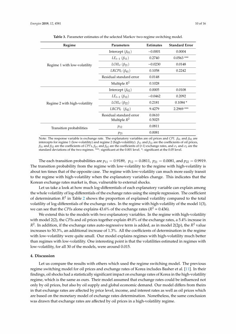
We also examine how the explanatory variables influence the exchange rates in each regime, based on the selected best model 2(2p). Table 3 presents the parameter estimates for both regimes. The volatility of regime 2 with high-volatility (𝜎 = 0.0610) was about four times that of regime 1 with low-volatility (𝜎 = 0.0148). In regime 1 with low-volatility, Korean exchange rates were not significantly influenced by any of the explanatory variables, but had positive dependence on their auto-regressive term (p < 0.001). In regime 2 with high-volatility, the variable 𝐿𝑂𝐼𝐿 positively influenced the exchange rates (p < 0.05) and the variable 𝐿𝑅𝐶𝑃𝐼 positively influenced the exchange rates to a much greater extent (p < 0.001). This shows that the exchange rates increase as oil prices or 𝐶𝑃𝐼s increase when the exchange rates markets are highly volatile. We observe that, in a highly volatile market, the exchange rates are significantly influenced by 𝐶𝑃𝐼s and oil prices but have no significant relationship with their auto-regressive terms. In a low-volatility market, only the auto-regressive terms are significant.

Table 3. Parameter estimates of the selected Markov two-regime switching model.

Regime Parameters Estimates Standard Error

Regime 1 with low-volatility

Intercept (𝛽 ) −0.0001 0.0004 𝐿𝐸 (𝛽 ) 0.2740 0.0563 *** 𝐿𝑂𝐼𝐿 (𝛽 ) −0.0230 0.0148 𝐿𝑅𝐶𝑃𝐼 (𝛽 ) 0.1058 0.2242

Figure 2. (a) The filtered probabilities of being in regime 1 and regime 2, estimated from the MRSM forthe exchange rates along with both oil prices and CPIs. The upper plot corresponds to the regime 1with low-volatility, and the lower plot corresponds to the regime 2 with high-volatility. (b) Volatilityplot of regime 1. (c) Volatility plot of regime 2.

We also examine how the explanatory variables influence the exchange rates in each regime,based on the selected best model 2(2p). Table 3 presents the parameter estimates for both regimes.The volatility of regime 2 with high-volatility (σ2 = 0.0610) was about four times that of regime1 with low-volatility (σ1 = 0.0148). In regime 1 with low-volatility, Korean exchange rates werenot significantly influenced by any of the explanatory variables, but had positive dependence ontheir auto-regressive term (p < 0.001). In regime 2 with high-volatility, the variable LOIL positivelyinfluenced the exchange rates (p < 0.05) and the variable LRCPI positively influenced the exchangerates to a much greater extent (p < 0.001). This shows that the exchange rates increase as oil prices orCPIs increase when the exchange rates markets are highly volatile. We observe that, in a highly volatilemarket, the exchange rates are significantly influenced by CPIs and oil prices but have no significantrelationship with their auto-regressive terms. In a low-volatility market, only the auto-regressive termsare significant.

Energies 2019, 12, 4581 10 of 16

Table 3. Parameter estimates of the selected Markov two-regime switching model.

Regime Parameters Estimates Standard Error

Regime 1 with low-volatility

Intercept (β01) −0.0001 0.0004

LEt−1 (β11) 0.2740 0.0563 ***

LOILt (β21) −0.0230 0.0148

LRCPIt (β41) 0.1058 0.2242

Residual standard error 0.0148

Multiple R2 0.1028

Regime 2 with high-volatility

Intercept (β02) 0.0005 0.0108

LEt−1 (β12) −0.0462 0.2092

LOILt (β22) 0.2181 0.1084 *

LRCPIt (β42) 9.4279 2.2969 ***

Residual standard error 0.0610Multiple R2 0.5025

Transition probabilities p12 0.0811

p21 0.0081

Note: The response variable is exchange rate. The explanatory variables are oil prices and CPI. β01 and β02 areintercepts for regime 1 (low-volatility) and regime 2 (high-volatility). β11 and β12 are the coefficients of oil prices,β21 and β22 are the coefficients of CPI’s, βp1 and βp2 are the coefficients of (t-1) exchange rates, and σ1 and σ2 are thestandard deviations of the two regimes. ***: significant at the 0.001 level. *: significant at the 0.05 level.

The each transition probabilities are p11 = 0.9189, p12 = 0.0811, p21 = 0.0081, and p22 = 0.9919.The transition probability from the regime with low-volatility to the regime with high-volatility isabout ten times that of the opposite case. The regime with low-volatility can much more easily transitto the regime with high-volatility when the explanatory variables change. This indicates that theKorean exchange rates market is, thus, vulnerable to external shocks.

Let us take a look at how much log-differentials of each explanatory variable can explain amongthe whole volatility of log-differentials of the exchange rates using the simple regression. The coefficientof determination R2 in Table 2 shows the proportion of explained volatility compared to the totalvolatility of log-differentials of the exchange rates. In the regime with high-volatility of the model 1(3),we can see that the CPIs alone explains 43.6% of the exchange rates (R2 = 0.436).

We extend this to the models with two explanatory variables. In the regime with high-volatilitywith model 2(2), the CPIs and oil prices together explain 49.0% of the exchange rates, a 5.4% increase inR2. In addition, if the exchange rates auto-regressive term is added, as in model 2(2p), the R2 valueincreases to 50.3%, an additional increase of 1.3%. All the coefficients of determination in the regimewith low-volatility were quite small. Our model explains regimes with high-volatility much betterthan regimes with low-volatility. One interesting point is that the volatilities estimated in regimes withlow-volatility, for all 30 of the models, were around 0.015.

4. Discussion

Let us compare the results with others which used the regime switching model. The previousregime switching model for oil prices and exchange rates of Korea includes Basher et al. [11]. In theirfindings, oil shocks had a statistically significant impact on exchange rates of Korea in the high-volatilityregime, which is the same as ours. Their model assumed that exchange rates could be influenced notonly by oil prices, but also by oil supply and global economic demand. Our model differs from theirsin that exchange rates are affected by price level, income, and interest rates as well as oil prices whichare based on the monetary model of exchange rates determination. Nonetheless, the same conclusionwas drawn that exchange rates are affected by oil prices in a high-volatility regime.

Energies 2019, 12, 4581 11 of 16

In Table 4, the auto-regression model without regime switching is also fitted for comparison. R2 inthe model is 0.247, which is much less than 0.503 in the high-volatility regime. LRCPI is significant (p <

0.01) but oil prices are not (p > 0.1). In the absence of regime switching, only LRCPI and auto-regressiveterms affect the Korean exchange rates. In other words, oil prices do not appear to affect the exchangerates, which is different from the results with MRSM. In the presence of Markov regime switching, oilprices significantly affect the exchange rates in the unstable regime. Thus, in models without Markovregime switching, the behavior in the stable regime overwhelms the behavior in the unstable regime.Korea has experienced two major economic crises, the Asian financial crisis and the global financialcrisis, which are precisely detected by the MRSM. Therefore, it can be seen from this study that stablemanagement of oil prices is essential for stabilizing exchange rates in these economic crises.

Table 4. Parameter estimates without the regime switching model.

Parameters Estimates Standard Error

Intercept (β01) −0.0003 0.0015LEt−1(β11) 0.3969 0.0535 ***LOILt (β21) 0.0225 0.0226

LRCPIt (β41) 0.3442 0.3649 ***Residual standard error 0.0266

Multiple R2 0.2475

Note: ***: significant at the 0.001 level.

A long period time series data in this research often contains more than two different trendsthroughout the whole time period. We fit the two-regime MRSM, which estimates separateauto-regression models with AR (1) in each regime and the volatility state at each time point can switchbetween the two regimes according to the behavior of a Markov process.

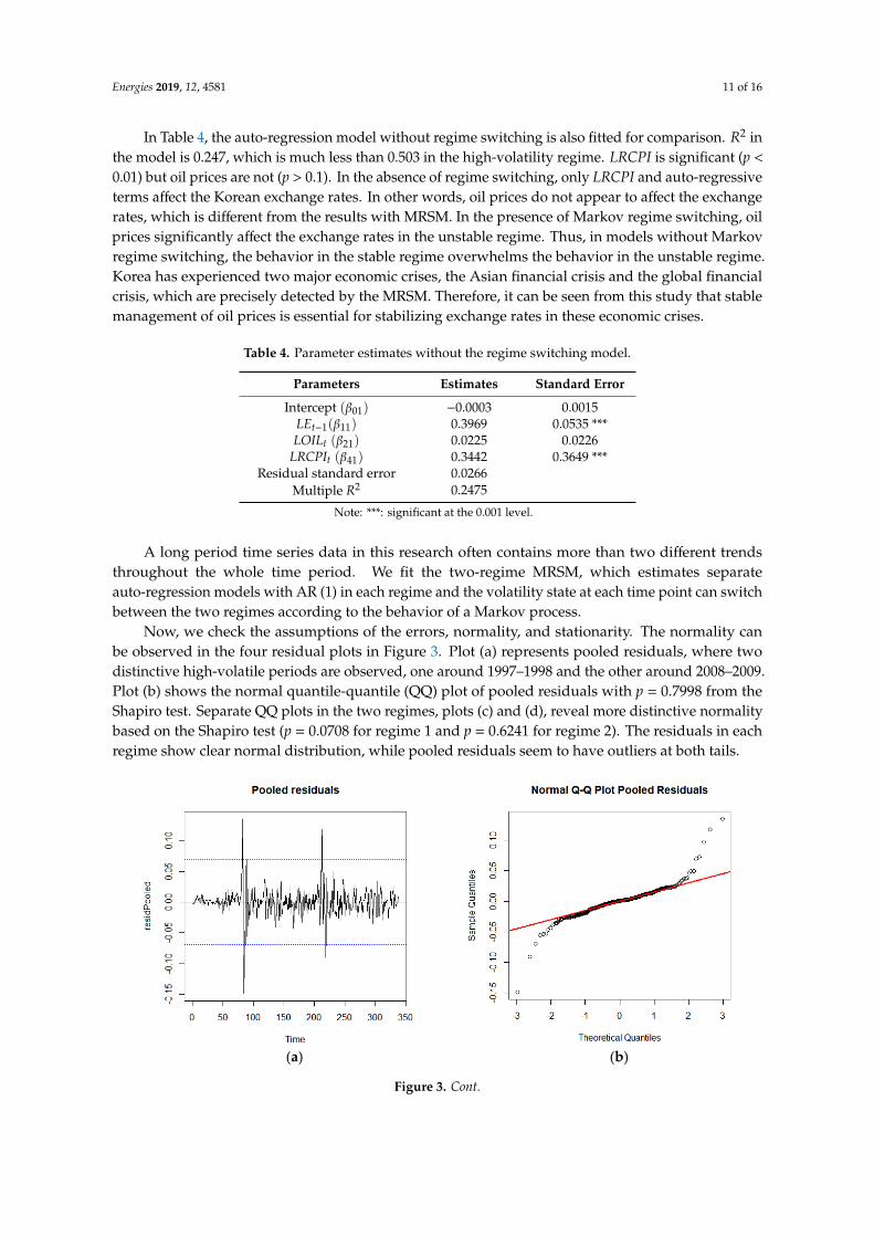
Now, we check the assumptions of the errors, normality, and stationarity. The normality canbe observed in the four residual plots in Figure 3. Plot (a) represents pooled residuals, where twodistinctive high-volatile periods are observed, one around 1997–1998 and the other around 2008–2009.Plot (b) shows the normal quantile-quantile (QQ) plot of pooled residuals with p = 0.7998 from theShapiro test. Separate QQ plots in the two regimes, plots (c) and (d), reveal more distinctive normalitybased on the Shapiro test (p = 0.0708 for regime 1 and p = 0.6241 for regime 2). The residuals in eachregime show clear normal distribution, while pooled residuals seem to have outliers at both tails.

Energies 2019, 12, 4581 11 of 16

it can be seen from this study that stable management of oil prices is essential for stabilizing exchange rates in these economic crises.

Table 4. Parameter estimates without the regime switching model.

Parameters Estimates Standard Error Intercept (𝛽 ) −0.0003 0.0015 𝐿𝐸 (𝛽 ) 0.3969 0.0535 *** 𝐿𝑂𝐼𝐿 (𝛽 ) 0.0225 0.0226 𝐿𝑅𝐶𝑃𝐼 (𝛽 ) 0.3442 0.3649 ***

Residual standard error 0.0266 Multiple R2 0.2475

Note: ***: significant at the 0.001 level.

A long period time series data in this research often contains more than two different trends throughout the whole time period. We fit the two-regime MRSM, which estimates separate auto-regression models with AR (1) in each regime and the volatility state at each time point can switch between the two regimes according to the behavior of a Markov process.

Now, we check the assumptions of the errors, normality, and stationarity. The normality can be observed in the four residual plots in Figure 3. Plot (a) represents pooled residuals, where two distinctive high-volatile periods are observed, one around 1997–1998 and the other around 2008–2009. Plot (b) shows the normal quantile-quantile (QQ) plot of pooled residuals with p = 0.7998 from the Shapiro test. Separate QQ plots in the two regimes, plots (c) and (d), reveal more distinctive normality based on the Shapiro test (p = 0.0708 for regime 1 and p = 0.6241 for regime 2). The residuals in each regime show clear normal distribution, while pooled residuals seem to have outliers at both tails.

(a) (b)

Figure 3. Cont.

Energies 2019, 12, 4581 12 of 16Energies 2019, 12, 4581 12 of 16

(c) (d)

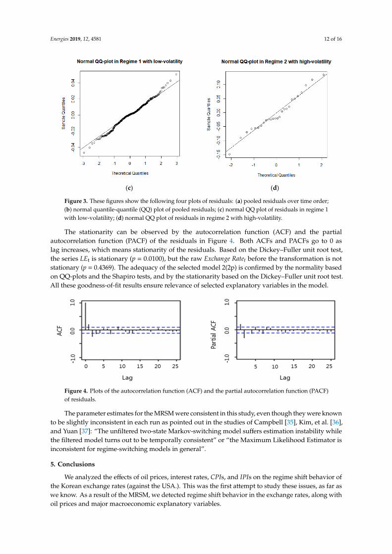
Figure 3. These figures show the following four plots of residuals: (a) pooled residuals over time order; (b) normal quantile-quantile (QQ) plot of pooled residuals; (c) normal QQ plot of residuals in regime 1 with low-volatility; (d) normal QQ plot of residuals in regime 2 with high-volatility.

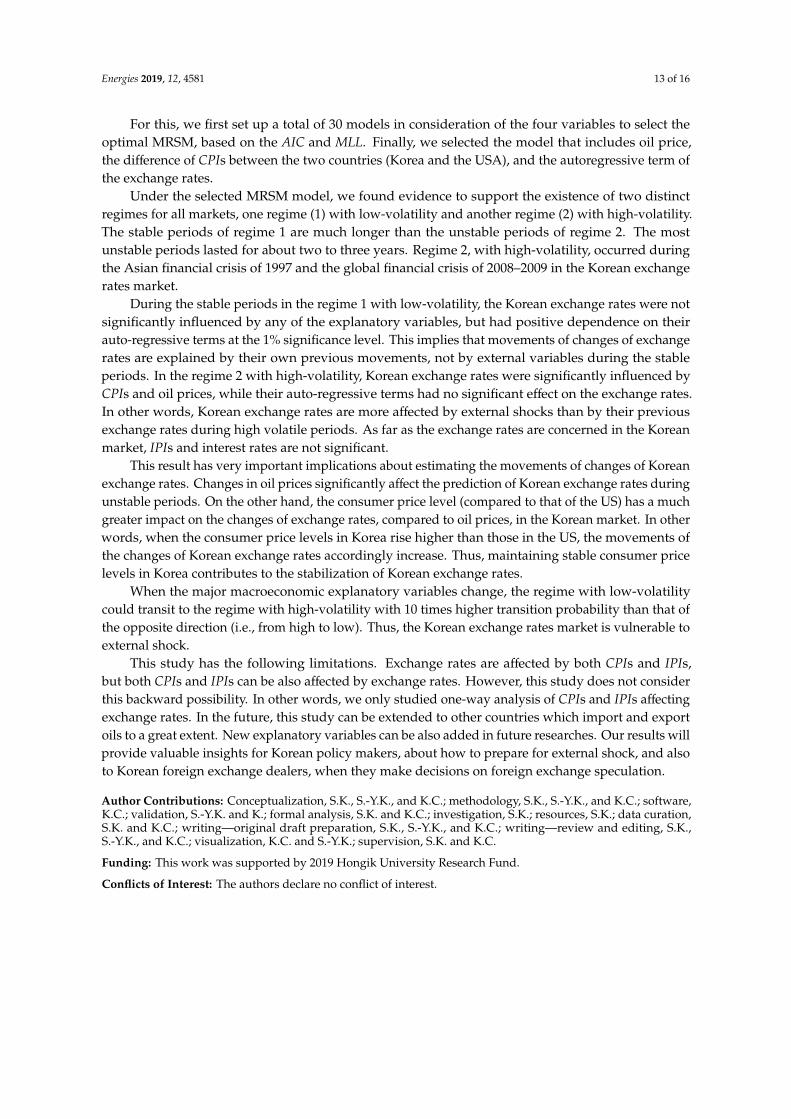
The stationarity can be observed by the autocorrelation function (ACF) and the partial autocorrelation function (PACF) of the residuals in Figure 4. Both ACFs and PACFs go to 0 as lag increases, which means stationarity of the residuals. Based on the Dickey–Fuller unit root test, the series 𝐿𝐸 is stationary (p = 0.0100), but the raw 𝐸𝑥𝑐ℎ𝑎𝑛𝑔𝑒 𝑅𝑎𝑡𝑒 before the transformation is not stationary (p = 0.4369). The adequacy of the selected model 2(2p) is confirmed by the normality based on QQ-plots and the Shapiro tests, and by the stationarity based on the Dickey–Fuller unit root test. All these goodness-of-fit results ensure relevance of selected explanatory variables in the model.

Figure 4. Plots of the autocorrelation function (ACF) and the partial autocorrelation function (PACF) of residuals.

The parameter estimates for the MRSM were consistent in this study, even though they were known to be slightly inconsistent in each run as pointed out in the studies of Campbell [35], Kim, et al. [36], and Yuan [37]: “The unfiltered two-state Markov-switching model suffers estimation instability while the filtered model turns out to be temporally consistent” or “the Maximum Likelihood Estimator is inconsistent for regime-switching models in general”.

5. Conclusions

We analyzed the effects of oil prices, interest rates, 𝐶𝑃𝐼s, and 𝐼𝑃𝐼s on the regime shift behavior of the Korean exchange rates (against the USA.). This was the first attempt to study these issues, as far as we know. As a result of the MRSM, we detected regime shift behavior in the exchange rates, along with oil prices and major macroeconomic explanatory variables.

Figure 3. These figures show the following four plots of residuals: (a) pooled residuals over time order;(b) normal quantile-quantile (QQ) plot of pooled residuals; (c) normal QQ plot of residuals in regime 1with low-volatility; (d) normal QQ plot of residuals in regime 2 with high-volatility.

The stationarity can be observed by the autocorrelation function (ACF) and the partialautocorrelation function (PACF) of the residuals in Figure 4. Both ACFs and PACFs go to 0 aslag increases, which means stationarity of the residuals. Based on the Dickey–Fuller unit root test,the series LEt is stationary (p = 0.0100), but the raw Exchange Ratet before the transformation is notstationary (p = 0.4369). The adequacy of the selected model 2(2p) is confirmed by the normality basedon QQ-plots and the Shapiro tests, and by the stationarity based on the Dickey–Fuller unit root test.All these goodness-of-fit results ensure relevance of selected explanatory variables in the model.

Energies 2019, 12, 4581 12 of 16

(c) (d)

Figure 3. These figures show the following four plots of residuals: (a) pooled residuals over time order; (b) normal quantile-quantile (QQ) plot of pooled residuals; (c) normal QQ plot of residuals in regime 1 with low-volatility; (d) normal QQ plot of residuals in regime 2 with high-volatility.

The stationarity can be observed by the autocorrelation function (ACF) and the partial autocorrelation function (PACF) of the residuals in Figure 4. Both ACFs and PACFs go to 0 as lag increases, which means stationarity of the residuals. Based on the Dickey–Fuller unit root test, the series 𝐿𝐸 is stationary (p = 0.0100), but the raw 𝐸𝑥𝑐ℎ𝑎𝑛𝑔𝑒 𝑅𝑎𝑡𝑒 before the transformation is not stationary (p = 0.4369). The adequacy of the selected model 2(2p) is confirmed by the normality based on QQ-plots and the Shapiro tests, and by the stationarity based on the Dickey–Fuller unit root test. All these goodness-of-fit results ensure relevance of selected explanatory variables in the model.

Figure 4. Plots of the autocorrelation function (ACF) and the partial autocorrelation function (PACF) of residuals.

The parameter estimates for the MRSM were consistent in this study, even though they were known to be slightly inconsistent in each run as pointed out in the studies of Campbell [35], Kim, et al. [36], and Yuan [37]: “The unfiltered two-state Markov-switching model suffers estimation instability while the filtered model turns out to be temporally consistent” or “the Maximum Likelihood Estimator is inconsistent for regime-switching models in general”.

5. Conclusions

We analyzed the effects of oil prices, interest rates, 𝐶𝑃𝐼s, and 𝐼𝑃𝐼s on the regime shift behavior of the Korean exchange rates (against the USA.). This was the first attempt to study these issues, as far as we know. As a result of the MRSM, we detected regime shift behavior in the exchange rates, along with oil prices and major macroeconomic explanatory variables.

Figure 4. Plots of the autocorrelation function (ACF) and the partial autocorrelation function (PACF)of residuals.

The parameter estimates for the MRSM were consistent in this study, even though they were knownto be slightly inconsistent in each run as pointed out in the studies of Campbell [35], Kim, et al. [36],and Yuan [37]: “The unfiltered two-state Markov-switching model suffers estimation instability whilethe filtered model turns out to be temporally consistent” or “the Maximum Likelihood Estimator isinconsistent for regime-switching models in general”.

5. Conclusions

We analyzed the effects of oil prices, interest rates, CPIs, and IPIs on the regime shift behavior ofthe Korean exchange rates (against the USA.). This was the first attempt to study these issues, as far aswe know. As a result of the MRSM, we detected regime shift behavior in the exchange rates, along withoil prices and major macroeconomic explanatory variables.

Energies 2019, 12, 4581 13 of 16

For this, we first set up a total of 30 models in consideration of the four variables to select theoptimal MRSM, based on the AIC and MLL. Finally, we selected the model that includes oil price,the difference of CPIs between the two countries (Korea and the USA), and the autoregressive term ofthe exchange rates.

Under the selected MRSM model, we found evidence to support the existence of two distinctregimes for all markets, one regime (1) with low-volatility and another regime (2) with high-volatility.The stable periods of regime 1 are much longer than the unstable periods of regime 2. The mostunstable periods lasted for about two to three years. Regime 2, with high-volatility, occurred duringthe Asian financial crisis of 1997 and the global financial crisis of 2008–2009 in the Korean exchangerates market.

During the stable periods in the regime 1 with low-volatility, the Korean exchange rates were notsignificantly influenced by any of the explanatory variables, but had positive dependence on theirauto-regressive terms at the 1% significance level. This implies that movements of changes of exchangerates are explained by their own previous movements, not by external variables during the stableperiods. In the regime 2 with high-volatility, Korean exchange rates were significantly influenced byCPIs and oil prices, while their auto-regressive terms had no significant effect on the exchange rates.In other words, Korean exchange rates are more affected by external shocks than by their previousexchange rates during high volatile periods. As far as the exchange rates are concerned in the Koreanmarket, IPIs and interest rates are not significant.

This result has very important implications about estimating the movements of changes of Koreanexchange rates. Changes in oil prices significantly affect the prediction of Korean exchange rates duringunstable periods. On the other hand, the consumer price level (compared to that of the US) has a muchgreater impact on the changes of exchange rates, compared to oil prices, in the Korean market. In otherwords, when the consumer price levels in Korea rise higher than those in the US, the movements ofthe changes of Korean exchange rates accordingly increase. Thus, maintaining stable consumer pricelevels in Korea contributes to the stabilization of Korean exchange rates.

When the major macroeconomic explanatory variables change, the regime with low-volatilitycould transit to the regime with high-volatility with 10 times higher transition probability than that ofthe opposite direction (i.e., from high to low). Thus, the Korean exchange rates market is vulnerable toexternal shock.

This study has the following limitations. Exchange rates are affected by both CPIs and IPIs,but both CPIs and IPIs can be also affected by exchange rates. However, this study does not considerthis backward possibility. In other words, we only studied one-way analysis of CPIs and IPIs affectingexchange rates. In the future, this study can be extended to other countries which import and exportoils to a great extent. New explanatory variables can be also added in future researches. Our results willprovide valuable insights for Korean policy makers, about how to prepare for external shock, and alsoto Korean foreign exchange dealers, when they make decisions on foreign exchange speculation.

Author Contributions: Conceptualization, S.K., S.-Y.K., and K.C.; methodology, S.K., S.-Y.K., and K.C.; software,K.C.; validation, S.-Y.K. and K.; formal analysis, S.K. and K.C.; investigation, S.K.; resources, S.K.; data curation,S.K. and K.C.; writing—original draft preparation, S.K., S.-Y.K., and K.C.; writing—review and editing, S.K.,S.-Y.K., and K.C.; visualization, K.C. and S.-Y.K.; supervision, S.K. and K.C.

Funding: This work was supported by 2019 Hongik University Research Fund.

Conflicts of Interest: The authors declare no conflict of interest.

Energies 2019, 12, 4581 14 of 16

Appendix A

Table A1. The Markov Regime Switching Models for exchange rates along with oil prices, interestrates, CPI’s and IPI’s.

Model Number Equation

1(1) LEt∣∣∣st = β0st + β2st LOILt + εt

∣∣∣st

1(1p) LEt∣∣∣st = β0st + β1st LEt−1 + β2st LOILt + εt

∣∣∣st

1(2) LEt∣∣∣st = β0st + β3st LRINTt + εt

∣∣∣st

1(2p) LEt∣∣∣st = β0st + β1st LEt−1 + β3st LRINTt + εt

∣∣∣st

1(3) LEt∣∣∣st = β0st + β4st LRCPIt + εt

∣∣∣st

1(3p) LEt∣∣∣st = β0st + β1st LEt−1 + β4st LRCPIt + εt

∣∣∣st

1(4) LEt∣∣∣st = β0st + β5st LRIPIt + εt

∣∣∣st

1(4p) LEt∣∣∣st = β0st + β1st LEt−1 + β5st LRIPIt + εt

∣∣∣st

2(1) LEt∣∣∣st = β0st + β2st LOILt + β3st LRINTt + εt

∣∣∣st

2(1p) LEt∣∣∣st = β0st + β1st LEt−1 + β2st LOILt + β3st LRINTt + εt

∣∣∣st

2(2) LEt∣∣∣st = β0st + β2st LOILt + β4st LRCPIt + εt

∣∣∣st

2(2p) LEt∣∣∣st = β0st + β1st LEt−1 + β2st LOILt + β4st LRCPIt + εt

∣∣∣st

2(3) LEt∣∣∣st = β0st + β2st LOILt + β5st LRIPIt + εt

∣∣∣st

2(3p) LEt∣∣∣st = β0st + β1st LEt−1 + β2st LOILt + β5st LRIPIt + εt

∣∣∣st

2(4) LEt∣∣∣st = β0st + β3st LRINTt + β4st LRCPIt + εt

∣∣∣st

2(4p) LEt∣∣∣st = β0st + β1st LEt−1 + β3st LRINTt + β4st LRCPIt + εt

∣∣∣st

2(5) LEt∣∣∣st = β0st + β3st LRINTt + β5st LRIPIt + εt

∣∣∣st

2(5p) LEt∣∣∣st = β0st + β1st LEt−1 + β3st LRINTt + β5st LRIPIt + εt

∣∣∣st

2(6) LEt∣∣∣st = β0st + β4st LRCPIt + β5st LRIPIt + εt

∣∣∣st

2(6p) LEt∣∣∣st = β0st + β1st LEt−1 + β4st LRCPIt + β5st LRIPIt + εt

∣∣∣st

3(1) LEt∣∣∣st = β0st + β2st LOILt + β3st LRINTt + β4st LRCPIt + εt

∣∣∣st

3(1p) LEt∣∣∣st = β0st + β1st LEt−1 + β2st LOILt + β3st LRINTt + β4st LRCPIt + εt

∣∣∣st

3(2) LEt∣∣∣st = β0st + β2st LOILt + β3st LRINTt + β5st LRIPIt + εt

∣∣∣st

3(2p) LEt∣∣∣st = β0st + β1st LEt−1 + β2st LOILt + β3st LRINTt + β5st LRIPIt + εt

∣∣∣st

3(3) LEt∣∣∣st = β0st + β2st LOILt + β4st LRCPIt + β5st LRIPIt + εt

∣∣∣st

3(3p) LEt∣∣∣st = β0st e + β1st LEt−1 + β2st LOILt + β4st LRCPIt + β5st LRIPIt + εt

∣∣∣st

3(4) LEt∣∣∣st = β0st + β3st LRINTt + β4st LRCPIt + β5st LRIPIt + εt

∣∣∣st

3(4p) LEt∣∣∣st = β0st + β1st LEt−1 + β3st LRINTt + β4st LRCPIt + β5st LRIPIt + εt

∣∣∣st

4(1) LEt∣∣∣st = β0st + β2st LOILt + β3st LRINTt + β4st LRCPIt + β5st LRIPIt + εt

∣∣∣st

4(1p) LEt∣∣∣st = β0st + β1st LEt−1 + β2st LOILt + β3st LRINTt + β4st LRCPIt + β5st LRIPIt + εt

∣∣∣st

References

1. Amano, R.; Van Norden, S. Exchange rates and oil price. Rev. Int. Econ. 1998, 6, 683–694. [CrossRef]2. Amano, R.; Van Norden, S. Oil prices and the rise and fall of the US real exchange rate. J. Int. Money Financ.

1998, 17, 299–316. [CrossRef]3. Chaudhuri, K.; Daniel, B. Long-Run equilibrium real exchange rates and oil prices. Econ. Lett. 1998, 58,

231–238. [CrossRef]4. Chen, S.S.; Chen, H.C. Oil prices and real exchange rates. Energy Econ. 2007, 29, 390–404. [CrossRef]5. Lizardo, R.A.; Mollick, A.V. Oil price fluctuations and US dollar exchange rate. Energy Econ. 2010, 32,

399–408. [CrossRef]6. Basher, S.A.; Haug, A.A.; Sadorsky, P. Oil prices, exchange rates and emerging stock markets. Energy Econ.

2012, 34, 227–240. [CrossRef]

Energies 2019, 12, 4581 15 of 16

7. Aloui, R.; Ben Aissa, M.S.; Nguyen, D.K. Conditional dependence structure between oil prices and exchangerates: A copula-GARCH approach. J. Int. Money Financ. 2013, 32, 719–738. [CrossRef]

8. Chen, W.P.; Choudhry, T.; Wu, C.C. The extreme value in crude oil and US dollar markets. J. Int. Money Financ.2013, 36, 191–210. [CrossRef]

9. Volkov, N.I.; Yuhn, K.H. Oil price shocks and exchange rate movements. Glob. Financ. J. 2016, 31, 18–30.[CrossRef]

10. Chen, H.; Liu, L.; Wang, Y.; Zhu, Y. Oil price shocks and US dollar exchange rates. Energy 2016, 112, 1036–1048.[CrossRef]

11. Basher, S.A.; Haug, A.A.; Sadorsky, P. The impact of oil shocks on exchange rates: A Markov-Switchingapproach. Energy Econ. 2016, 54, 11–23. [CrossRef]

12. Yang, L.; Cai, X.J.; Hamori, S. Does the crude oil influence the exchange rates of oil importing and oil exportingcountries differently? A wavelet coherence analysis. Int. Rev. Econ. Financ. 2017, 49, 536–547. [CrossRef]

13. Hamilton, J.D. A new approach to the economic analysis of nonstationary time series and the business cycle.Econometrica 1989, 57, 357–384. [CrossRef]

14. Cai, J. A Markov model of unconditional variance in ARCH. J. Bus. Econ. Stat. 1994, 12, 309–316.15. Gray, S.F. An Analysis of Conditional Regime-Switching Models; Working Paper; Fuqua School of Business,

Duke University: Durham, NC, USA, 1995.16. Henry, O.T. Regime switching in the relationship between equity returns and short-Term interest rates in the

UK. J. Bank. Financ. 2009, 33, 405–414. [CrossRef]17. Kim, S.; Kim, S.Y.; Choi, K. Markov Regime-Switching Models for Stock Returns Along with Exchange Rates

and Interest Rates in Korea. Notes Electr. Eng. 2017, 461, 253–259.18. Kim, S.; Kim, S.Y.; Choi, K. Modeling and analysis for stock return movements along with exchange rates

and interest rates in Markov regime-Switching models. Clust. Comput. 2019, 22, 2039–2048. [CrossRef]19. Frenkel, J.A. A Monetary Approach to the Exchange Rate: Doctrinal Aspects and Empirical Evidence. Scand. J.

Econ. 1976, 78, 200–224. [CrossRef]20. Mussa, M. The Exchange Rate, the Balance of Payments and Monetary and Fiscal Policy under a Regime of

Controlled Floating. Scand. J. Econ. 1976, 78, 229–248. [CrossRef]21. Mussa, M. Empirical Regularities in the Behavior of Exchange Rates and Theories of the Foreign Exchange

Market. In Carnegie-Rochester Conference Series on Public Policy: Policies for Employment, Prices and ExchangeRates; Brunner, K., Meltzer, A.H., Eds.; North Holland: Amsterdam, The Netherlands, 1979; Volume 11,pp. 9–57.

22. Mussa, M. The theory of Exchange Rate Determination. In Exchange Rate Theory and Practice; Bilson, J.F.O.,Marston, R.C., Eds.; University of Chicago Press: Chicago, IL, USA, 1984; pp. 13–78.

23. Bilson, J.F.O. Rational Expectations and the Exchange Rate. In The Economics of Exchange Rates: SelectedStudies; Frenkel, J.A., Johnson, H.G., Eds.; Addison-Wesley Press: Boston, MA, USA, 1978.

24. Meese, R.A.; Kenneth, R. Empirical Exchange Rate Models of the Seventies: Do They Fit Out of Sample?J. Int. Econ. 1983, 14, 3–24. [CrossRef]

25. Meese, R.A.; Kenneth, R. The Out-Of-Sample Failure of Empirical Exchange Rate Models: Sampling Error orMisspecification? In Exchange Rates and International Macroeconomics; Frenkel, J., Ed.; NBER and University ofChicago Press: Chicago, IL, USA, 1983.

26. Osborne, M.F.M. Brownian motion in the stock market. Oper. Res. 1959, 7, 145–273. [CrossRef]27. Ayodeji, I. A Three-State Markov-Modulated Switching Model for Exchange Rates. J. Math. 2016, 2016,

5061749. [CrossRef]28. Sanchez-Espigares, J.A.; Jose, A.L. MSwM Examples. 2018. Available online: https://cran.r-project.org/web/

packages/MSwM/vignettes/examples.pdf (accessed on 24 November 2019).29. Kuan, C.M. Lecture on the Markov Switching Model. Available online: http://homepage.ntu.edu.tw/~ckuan/

pdf/Lec-Markov_note_spring%202010.pdf (accessed on 24 November 2019).30. Akaike, H. A new Look at statistical model identification. IEEE Trans. Autom. Control 1974, 19, 716–723.

[CrossRef]31. Akaike, H. A Bayesian extension of the minimum AIC procedure. Biometrika 1979, 66, 237–242. [CrossRef]32. Pinheiro, J.C.; Bates, D.M. Mixed-Effects Models in S and S-Plus, 1st ed.; Springer: New York, NY, USA, 2000.33. Rice, J.A. Mathematical Statistics and Data Analysis, 3rd ed.; Thomson, Brooks/Cole: Belmont, CA, USA, 2007.34. Venables, W.N.; Ripley, B.D. Modern Applied Statistics with S, 4th ed.; Springer: New York, NY, USA, 2002.

Energies 2019, 12, 4581 16 of 16

35. Campbell, S.D. Specification Testing and Semiparametric Estimation of Regime Switching Models: An Examinationof the US Short Term Interest Rate; Working Paper 2002–26; Brown University Department of Economics:Providence, RI, USA, 2002.

36. Kim, C.J.; Piger, J.; Startz, R. Estimation of Markov regime-Switching regression models with endogenousswitching. J. Econom. 2008, 143, 263–273. [CrossRef]

37. Yuan, C. Forecasting Exchange Rates: The Multi-State Markov-Switching Model with Smoothing.Available online: http://economics.umbc.edu/files/2014/09/wp_09_115.pdf (accessed on 30 June 2017).

© 2019 by the authors. Licensee MDPI, Basel, Switzerland. This article is an open accessarticle distributed under the terms and conditions of the Creative Commons Attribution(CC BY) license (http://creativecommons.org/licenses/by/4.0/).