1 service scheduling algorithms. 2 outline zwhat is scheduling zwhy we need it zrequirements of a...

1

Service Scheduling Algorithms

2

Outline What is scheduling Why we need it Requirements of a scheduling discipline Fundamental choices Scheduling best effort connections Scheduling guaranteed-service connections Packet drop strategies

Scheduling

Sharing always results in contention A scheduling discipline resolves contention:

who’s next?

Key to fairly sharing resources and providing performance guarantees

Components

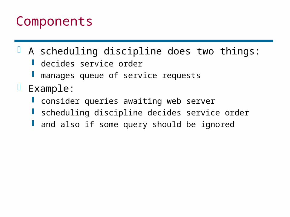
A scheduling discipline does two things: decides service order manages queue of service requests

Example: consider queries awaiting web server scheduling discipline decides service order and also if some query should be ignored

Where?

Anywhere where contention may occur At every layer of protocol stack Usually studied at network layer, at output

queues of switches

6


Why do we need one?

Because future applications need it We expect two types of future applications

best-effort (adaptive, non-real time) e.g. email, some types of file transfer

guaranteed service (non-adaptive, real time) e.g. packet voice, interactive video, stock quotes

What can scheduling disciplines do?

Give different users different qualities of service Example of passengers waiting to board a plane

early boarders spend less time waiting bumped off passengers are ‘lost’!

Scheduling disciplines can allocate bandwidth delay loss

They also determine how fair the network is

9


Requirements

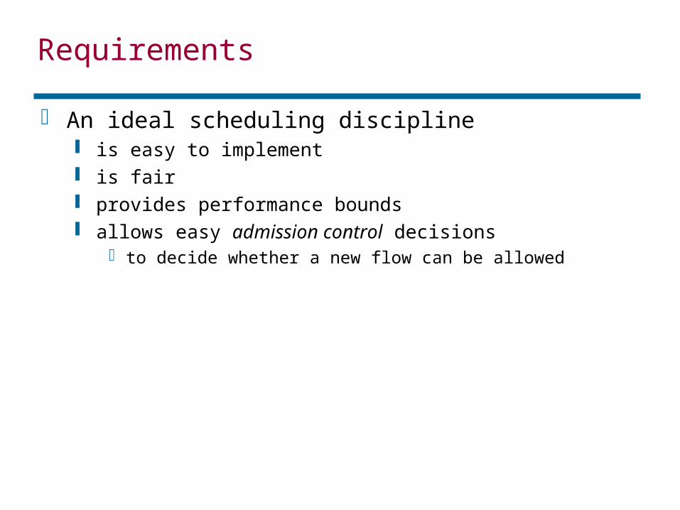
An ideal scheduling discipline is easy to implement is fair provides performance bounds allows easy admission control decisions

to decide whether a new flow can be allowed

Requirements: 1. Ease of implementation

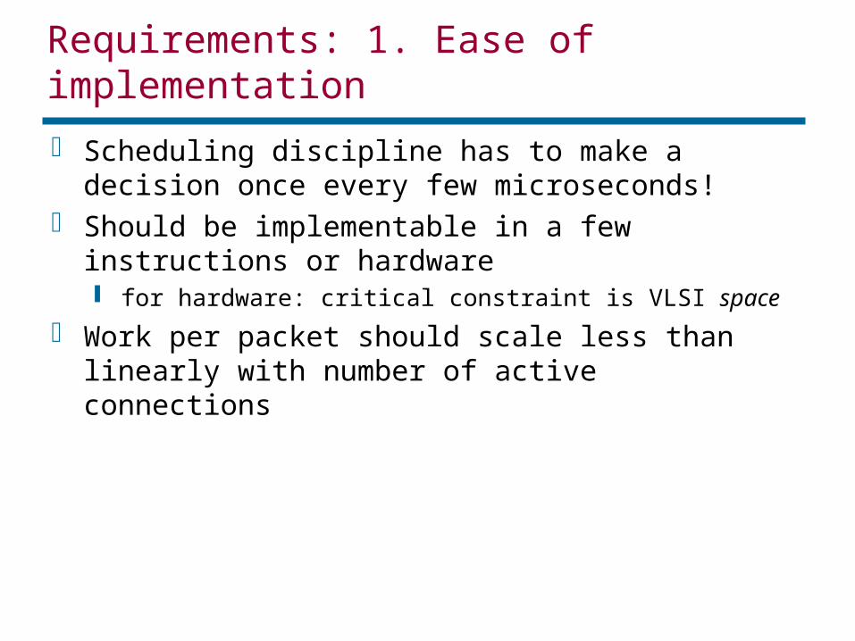
Scheduling discipline has to make a decision once every few microseconds!

Should be implementable in a few instructions or hardware for hardware: critical constraint is VLSI space

Work per packet should scale less than linearly with number of active connections

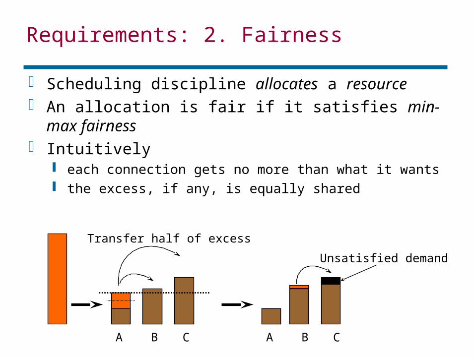
Requirements: 2. Fairness

Scheduling discipline allocates a resource An allocation is fair if it satisfies min-max fairness Intuitively

each connection gets no more than what it wants the excess, if any, is equally shared

A B C A B C

Transfer half of excess

Unsatisfied demand

Fairness (contd.)

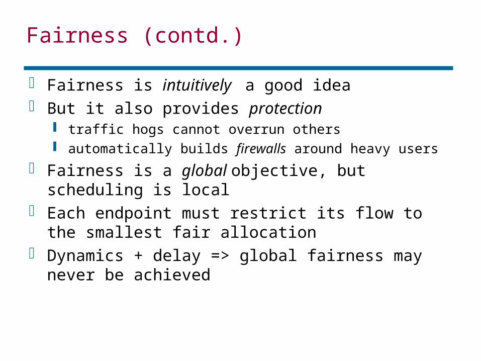
Fairness is intuitively a good idea But it also provides protection

traffic hogs cannot overrun others automatically builds firewalls around heavy users

Fairness is a global objective, but scheduling is local

Each endpoint must restrict its flow to the smallest fair allocation

Dynamics + delay => global fairness may never be achieved

Requirements: 3. Performance bounds

What is it? A way to obtain a desired level of service

Can be deterministic or statistical Common parameters are

bandwidth delay delay-jitter loss

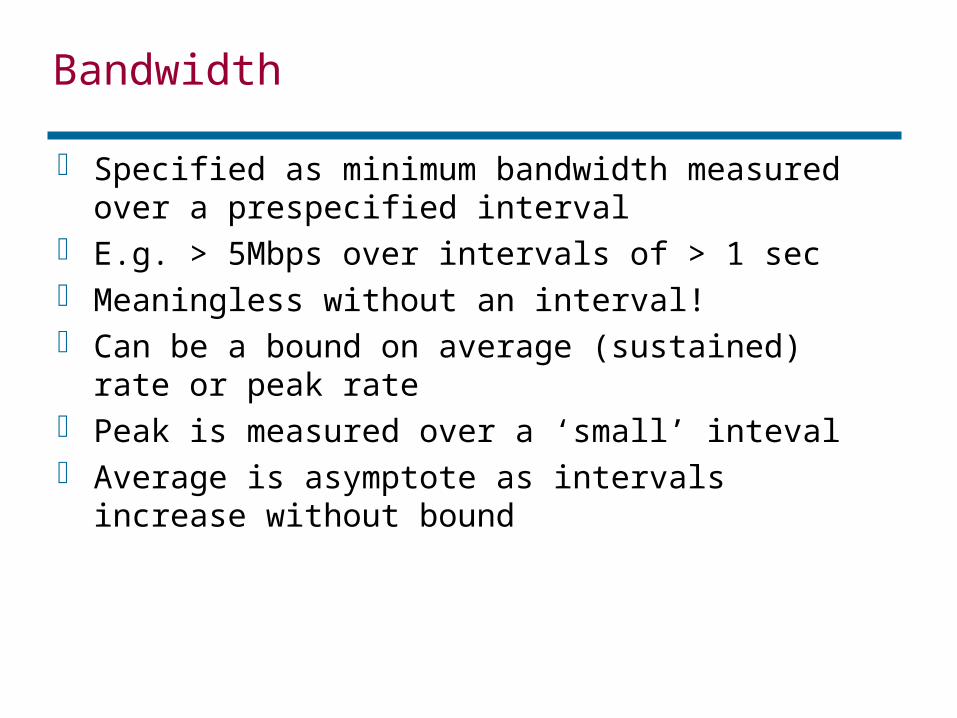
Bandwidth

Specified as minimum bandwidth measured over a prespecified interval

E.g. > 5Mbps over intervals of > 1 sec Meaningless without an interval! Can be a bound on average (sustained) rate or

peak rate Peak is measured over a ‘small’ inteval Average is asymptote as intervals increase

without bound

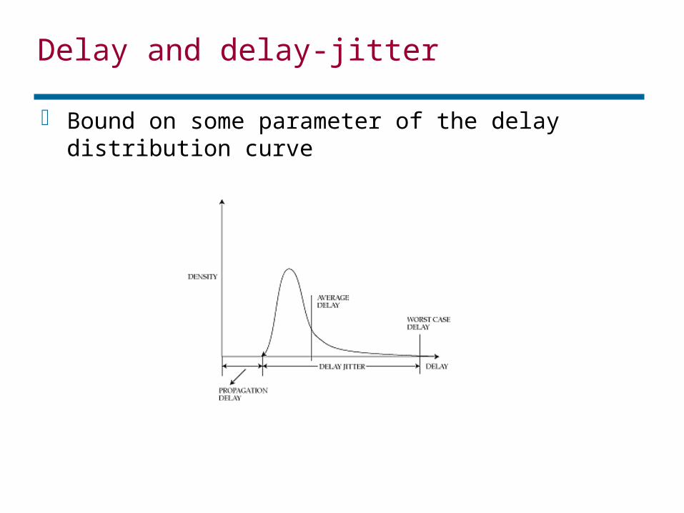
Delay and delay-jitter

Bound on some parameter of the delay distribution curve

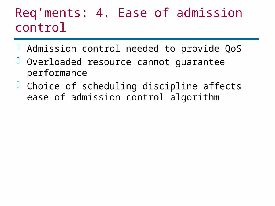
Req’ments: 4. Ease of admission control

Admission control needed to provide QoS Overloaded resource cannot guarantee

performance Choice of scheduling discipline affects ease of

admission control algorithm

18


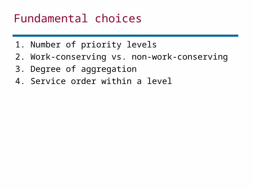
Fundamental choices

1. Number of priority levels2. Work-conserving vs. non-work-conserving3. Degree of aggregation4. Service order within a level

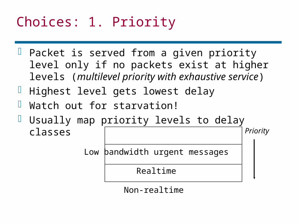
Choices: 1. Priority

Packet is served from a given priority level only if no packets exist at higher levels (multilevel priority with exhaustive service)

Highest level gets lowest delay Watch out for starvation! Usually map priority levels to delay classes

Low bandwidth urgent messages

Realtime

Non-realtime

Priority

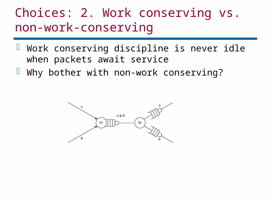
Choices: 2. Work conserving vs. non-work-conserving

Work conserving discipline is never idle when packets await service

Why bother with non-work conserving?

Non-work-conserving disciplines

Key conceptual idea: delay packet till eligible Reduces delay-jitter => fewer buffers in network How to choose eligibility time?

rate-jitter regulator bounds maximum outgoing rate

delay-jitter regulator compensates for variable delay at previous hop

Do we need non-work-conservation?

Can remove delay-jitter at an endpoint instead but also reduces size of switch buffers…

Increases mean delay not a problem for playback applications

Wastes bandwidth can serve best-effort packets instead

Always punishes a misbehaving source can’t have it both ways

Bottom line: not too bad, implementation cost may be the biggest problem

Choices: 3. Degree of aggregation

More aggregation less state cheaper

smaller VLSI less to advertise

BUT: less individualization

Solution aggregate to a class, members of class have same

performance requirement no protection within class

Choices: 4. Service within a priority level

In order of arrival (FCFS) or in order of a service tag

Service tags => can arbitrarily reorder queue Need to sort queue, which can be expensive

FCFS bandwidth hogs win (no protection) no guarantee on delays

Service tags with appropriate choice, both protection and delay

bounds possible

26


27

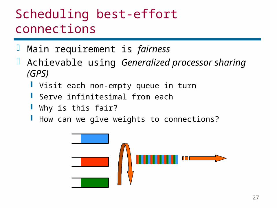
Scheduling best-effort connections Main requirement is fairness Achievable using Generalized processor sharing

(GPS) Visit each non-empty queue in turn Serve infinitesimal from each Why is this fair? How can we give weights to connections?

28

More on GPS GPS is unimplementable!

we cannot serve infinitesimals, only packets

No packet discipline can be as fair as GPS while a packet is being served, we are unfair to others

Degree of unfairness can be bounded Define: work(I,a,b) = # bits transmitted for

connection I in time [a,b] Absolute fairness bound for discipline S

Max (work_GPS(I,a,b) - work_S(I, a,b))

Relative fairness bound for discipline S Max (work_S(I,a,b) - work_S(J,a,b))

29

What next? We can’t implement GPS So, lets see how to emulate it We want to be as fair as possible But also have an efficient implementation

30

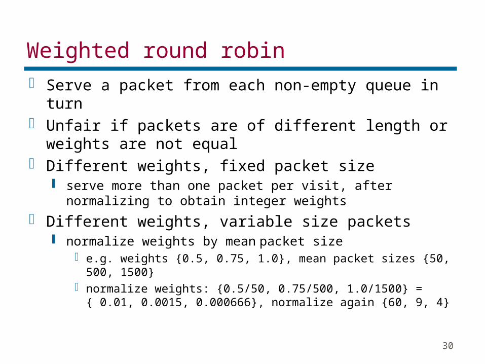
Weighted round robin Serve a packet from each non-empty queue in

turn Unfair if packets are of different length or weights

are not equal Different weights, fixed packet size

serve more than one packet per visit, after normalizing to obtain integer weights

Different weights, variable size packets normalize weights by mean packet size

e.g. weights {0.5, 0.75, 1.0}, mean packet sizes {50, 500, 1500}

normalize weights: {0.5/50, 0.75/500, 1.0/1500} = { 0.01, 0.0015, 0.000666}, normalize again {60, 9, 4}

31

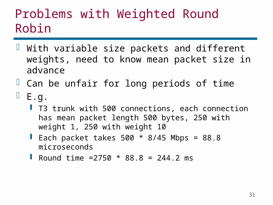
Problems with Weighted Round Robin With variable size packets and different weights,

need to know mean packet size in advance Can be unfair for long periods of time E.g.

T3 trunk with 500 connections, each connection has mean packet length 500 bytes, 250 with weight 1, 250 with weight 10

Each packet takes 500 * 8/45 Mbps = 88.8 microseconds

Round time =2750 * 88.8 = 244.2 ms

32

Weighted Fair Queueing (WFQ) Deals better with variable size packets and

weights GPS is fairest discipline Find the finish time of a packet, had we been

doing GPS Then serve packets in order of their finish times

33

WFQ: first cut Suppose, in each round, the server served one bit from

each active connection Round number is the number of rounds already completed

can be fractional If a packet of length p arrives to an empty queue when the

round number is R, it will complete service when the round number is R + p => finish number is R + p independent of the number of other connections!

If a packet arrives to a non-empty queue, and the previous packet has a finish number of f, then the packet’s finish number is f+p

Serve packets in order of finish numbers

34

A catch A queue may need to be considered non-empty

even if it has no packets in it e.g. packets of length 1 from connections A and B, on a

link of speed 1 bit/sec at time 1, packet from A served, round number = 0.5 A has no packets in its queue, yet should be considered

non-empty, because a packet arriving to it at time 1 should have finish number 1+ p

A connection is active if the last packet served from it, or in its queue, has a finish number greater than the current round number

35

WFQ continued To sum up, assuming we know the current round

number R Finish number of packet of length p

if arriving to active connection = previous finish number + p

if arriving to an inactive connection = R + p

(How should we deal with weights?) To implement, we need to know two things:

is connection active? if not, what is the current round number?

Answer to both questions depends on computing the current round number (why?)

36

WFQ: computing the round number Naively: round number = number of rounds of

service completed so far what if a server has not served all connections in a

round? what if new conversations join in halfway through a

round?

Redefine round number as a real-valued variable that increases at a rate inversely proportional to the number of currently active connections this takes care of both problems (why?)

With this change, WFQ emulates GPS instead of bit-by-bit RR

37

Problem: iterated deletion

A sever recomputes round number on each packet arrival At any recomputation, the number of conversations can go

up at most by one, but can go down to zero => overestimation Trick

use previous count to compute round number if this makes some conversation inactive, recompute repeat until no conversations become inactive

Round number # active conversations

38

WFQ implementation On packet arrival:

use source + destination address (or VCI) to classify it and look up finish number of last packet served (or waiting to be served)

recompute round number compute finish number insert in priority queue sorted by finish numbers if no space, drop the packet with largest finish number

On service completion select the packet with the lowest finish number

39

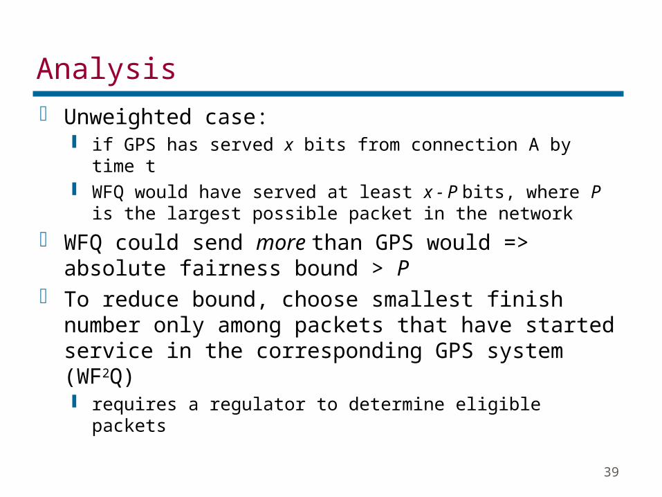
Analysis Unweighted case:

if GPS has served x bits from connection A by time t WFQ would have served at least x - P bits, where P is

the largest possible packet in the network

WFQ could send more than GPS would => absolute fairness bound > P

To reduce bound, choose smallest finish number only among packets that have started service in the corresponding GPS system (WF2Q) requires a regulator to determine eligible packets

40

Evaluation Pros

like GPS, it provides protection can obtain worst-case end-to-end delay bound gives users incentive to use intelligent flow control (and

also provides rate information implicitly)

Cons needs per-connection state iterated deletion is complicated requires a priority queue

41


42

Scheduling guaranteed-service connections

With best-effort connections, goal is fairness With guaranteed-service connections

what performance guarantees are achievable? how easy is admission control?

We now study some scheduling disciplines that provide performance guarantees

43

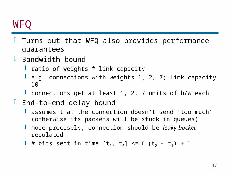
WFQ Turns out that WFQ also provides performance

guarantees Bandwidth bound

ratio of weights * link capacity e.g. connections with weights 1, 2, 7; link capacity 10 connections get at least 1, 2, 7 units of b/w each

End-to-end delay bound assumes that the connection doesn’t send ‘too much’

(otherwise its packets will be stuck in queues) more precisely, connection should be leaky-bucket

regulated # bits sent in time [t1, t2] <= (t2 - t1) +

44

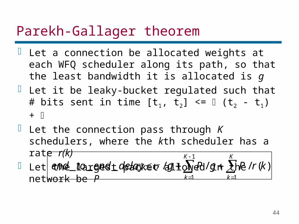
Parekh-Gallager theorem Let a connection be allocated weights at each

WFQ scheduler along its path, so that the least bandwidth it is allocated is g

Let it be leaky-bucket regulated such that # bits sent in time [t1, t2] <= (t2 - t1) +

Let the connection pass through K schedulers, where the kth scheduler has a rate r(k)

Let the largest packet allowed in the network be P

1

1 1

)(///___K

k

K

k

krPgPgdelayendtoend

45

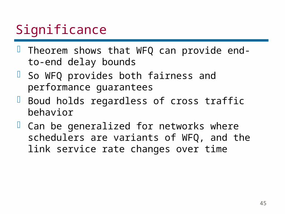
Significance Theorem shows that WFQ can provide end-to-end

delay bounds So WFQ provides both fairness and performance

guarantees Boud holds regardless of cross traffic behavior Can be generalized for networks where

schedulers are variants of WFQ, and the link service rate changes over time

46

Problems To get a delay bound, need to pick g

the lower the delay bounds, the larger g needs to be large g => exclusion of more competitors from link g can be very large, in some cases 80 times the peak

rate!

Sources must be leaky-bucket regulated but choosing leaky-bucket parameters is problematic

WFQ couples delay and bandwidth allocations low delay requires allocating more bandwidth wastes bandwidth for low-bandwidth low-delay sources

47

Delay-Earliest Due Date Earliest-due-date: packet with earliest deadline selected Delay-EDD prescribes how to assign deadlines to packets A source is required to send slower than its peak rate Bandwidth at scheduler reserved at peak rate Deadline = expected arrival time + delay bound

If a source sends faster than contract, delay bound will not apply

Each packet gets a hard delay bound Delay bound is independent of bandwidth requirement

but reservation is at a connection’s peak rate Implementation requires per-connection state and a

priority queue

48

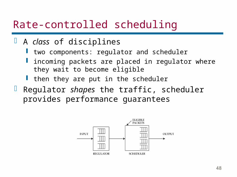
Rate-controlled scheduling A class of disciplines

two components: regulator and scheduler incoming packets are placed in regulator where they

wait to become eligible then they are put in the scheduler

Regulator shapes the traffic, scheduler provides performance guarantees

49

Examples Recall

rate-jitter regulator bounds maximum outgoing rate

delay-jitter regulator compensates for variable delay at previous hop

Rate-jitter regulator + FIFO similar to Delay-EDD (what is the difference?)

Rate-jitter regulator + multi-priority FIFO gives both bandwidth and delay guarantees (RCSP)

Delay-jitter regulator + EDD gives bandwidth, delay,and delay-jitter bounds (Jitter-

EDD)

50

Analysis First regulator on path monitors and regulates

traffic => bandwidth bound End-to-end delay bound

delay-jitter regulator reconstructs traffic => end-to-end delay is fixed (= worst-

case delay at each hop) rate-jitter regulator

partially reconstructs traffic can show that end-to-end delay bound is smaller than (sum

of delay bound at each hop + delay at first hop)

51

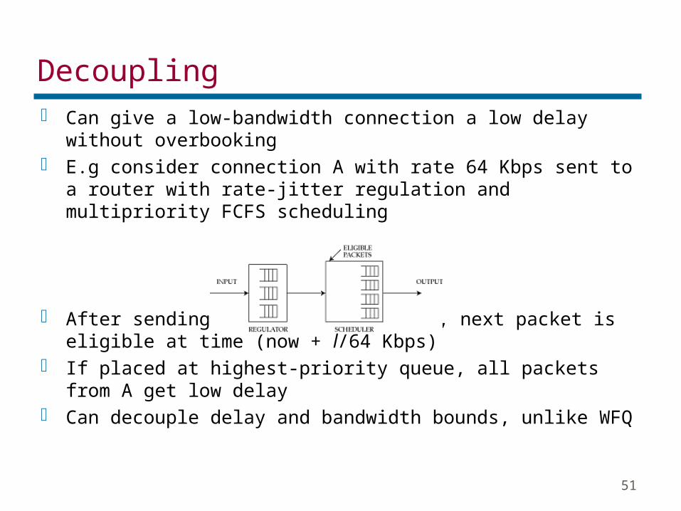
Decoupling Can give a low-bandwidth connection a low delay without

overbooking E.g consider connection A with rate 64 Kbps sent to a

router with rate-jitter regulation and multipriority FCFS scheduling

After sending a packet of length l, next packet is eligible at time (now + l/64 Kbps)

If placed at highest-priority queue, all packets from A get low delay

Can decouple delay and bandwidth bounds, unlike WFQ

52

Evaluation Pros

flexibility: ability to emulate other disciplines can decouple bandwidth and delay assignments end-to-end delay bounds are easily computed do not require complicated schedulers to guarantee

protection can provide delay-jitter bounds

Cons require an additional regulator at each output port delay-jitter bounds at the expense of increasing mean

delay delay-jitter regulation is expensive (clock synch,

timestamps)

53

Summary Two sorts of applications: best effort and

guaranteed service Best effort connections require fair service

provided by GPS, which is unimplementable emulated by WFQ and its variants

Guaranteed service connections require performance guarantees provided by WFQ, but this is expensive may be better to use rate-controlled schedulers

54


55

Packet dropping Packets that cannot be served immediately are

buffered Full buffers => packet drop strategy Packet losses happen almost always from best-

effort connections (why?) Shouldn’t drop packets unless imperative

packet drop wastes resources (why?)

56

Classification of drop strategies

1. Degree of aggregation2. Drop priorities3. Early or late4. Drop position

57

1. Degree of aggregation Degree of discrimination in selecting a packet to

drop E.g. in vanilla FIFO, all packets are in the same

class Instead, can classify packets and drop packets

selectively The finer the classification the better the

protection Max-min fair allocation of buffers to classes

drop packet from class with the longest queue (why?)

58

2. Drop priorities Drop lower-priority packets first How to choose?

endpoint marks packets regulator marks packets congestion loss priority (CLP) bit in packet header

59

CLP bit: pros and cons Pros

if network has spare capacity, all traffic is carried during congestion, load is automatically shed

Cons separating priorities within a single connection is hard what prevents all packets being marked as high

priority?

60

2. Drop priority (contd.) Special case of AAL5

want to drop an entire frame, not individual cells cells belonging to the selected frame are preferentially

dropped

Drop packets from ‘nearby’ hosts first because they have used the least network resources can’t do it on Internet because hop count (TTL)

decreases

61

3. Early vs. late drop Early drop => drop even if space is available

signals endpoints to reduce rate cooperative sources get lower overall delays,

uncooperative sources get severe packet loss

Early random drop drop arriving packet with fixed drop probability if queue

length exceeds threshold intuition: misbehaving sources more likely to send

packets and see packet losses doesn’t work!

62

3. Early vs. late drop: RED Random early detection (RED) makes three improvements Metric is moving average of queue lengths

small bursts pass through unharmed only affects sustained overloads

Packet drop probability is a function of mean queue length prevents severe reaction to mild overload

Can mark packets instead of dropping them allows sources to detect network state without losses

RED improves performance of a network of cooperating TCP sources

No bias against bursty sources Controls queue length regardless of endpoint cooperation

63

4. Drop position Can drop a packet from head, tail, or random

position in the queue Tail

easy default approach

Head harder lets source detect loss earlier

64

4. Drop position (contd.) Random

hardest if no aggregation, hurts hogs most unlikely to make it to real routers

Drop entire longest queue easy almost as effective as drop tail from longest queue

1 service scheduling algorithms. 2 outline zwhat is scheduling zwhy we need it zrequirements of a...

Documents

scheduling disciplines

service connectionspacket

service orderand

fairnessscheduling discipline

nonreal timee

global fairness

network layer

performance boundswhat