1 self-optimizing control theory. 2 step s3: implementation of optimal operation optimal operation...
TRANSCRIPT

1
Self-optimizing control Theory

2
Step S3: Implementation of optimal operation
• Optimal operation for given d*:
minu J(u,x,d)subject to:
Model equations: f(u,x,d) = 0
Operational constraints: g(u,x,d) < 0
→ uopt(d*)
Problem: Usally cannot keep uopt constant because disturbances d change
How should we adjust the degrees of freedom (u)?
What should we control?

3
y
“Optimizing Control”
4
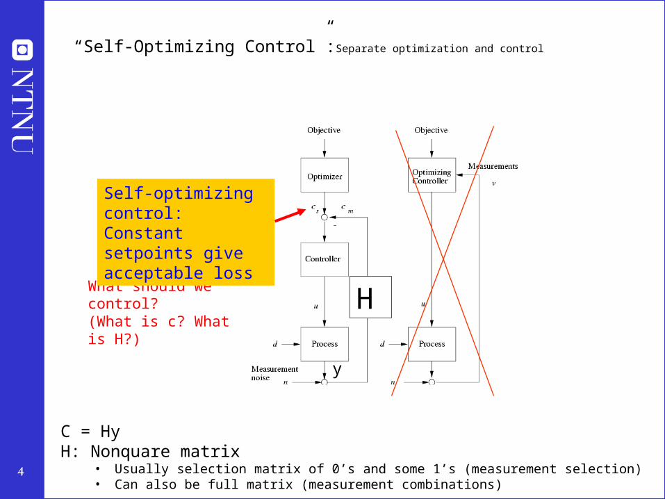
What should we control?(What is c? What is H?) H
y
C = HyH: Nonquare matrix
• Usually selection matrix of 0’s and some 1’s (measurement selection)• Can also be full matrix (measurement combinations)
“Self-Optimizing Control”:Separate optimization and control
Self-optimizing control: Constant setpoints give acceptable loss

5
Definition of self-optimizing control
“Self-optimizing control is when we achieve acceptable loss (in comparison with truly optimal operation) with constant setpoint values for the controlled variables (without the need to reoptimize when disturbances occur).”
Reference: S. Skogestad, “Plantwide control: The search for the self-optimizing control structure'', Journal of Process Control, 10, 487-507 (2000).
Acceptable loss ) self-optimizing control

6
Remarks “self-optimizing control”
1. Old idea (Morari et al., 1980):
“We want to find a function c of the process variables which when held constant, leads automatically to the optimal adjustments of the manipulated variables, and with it, the optimal operating conditions.”
2. “Self-optimizing control” = acceptable steady-state behavior with constant CVs.
“Self-regulation” = acceptable dynamic behavior with constant MVs.
3. Choice of good c (CV) is always important, even with RTO layer included
3. For unconstrained DOFs: Ideal self-optimizing variable is gradient, Ju = J/ u
– Keep gradient at zero for all disturbances (c = Ju=0)
– Problem: no measurement of gradient
7
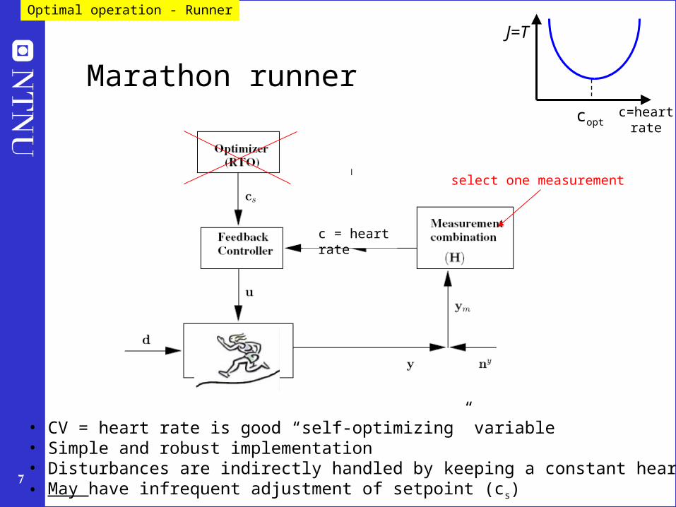
Marathon runner
c = heart rate
select one measurement
• CV = heart rate is good “self-optimizing” variable• Simple and robust implementation• Disturbances are indirectly handled by keeping a constant heart rate• May have infrequent adjustment of setpoint (cs)
Optimal operation - Runner
c=heart rate
J=T
copt

9
• Central bank. J = welfare. u = interest rate. c=inflation rate (2.5%)• Cake baking. J = nice taste, u = heat input. c = Temperature (200C)• Business, J = profit. c = ”Key performance indicator (KPI), e.g.
– Response time to order– Energy consumption pr. kg or unit– Number of employees– Research spendingOptimal values obtained by ”benchmarking”
• Investment (portofolio management). J = profit. c = Fraction of investment in shares (50%)
• Biological systems:– ”Self-optimizing” controlled variables c have been found by natural selection– Need to do ”reverse engineering” :
• Find the controlled variables used in nature• From this possibly identify what overall objective J the biological system has been
attempting to optimize
Further examples self-optimizing control
Define optimal operation (J) and look for ”magic” variable (c) which when kept constant gives acceptable loss (self-optimizing control)
Unconstrained degrees of freedom

10
The ideal “self-optimizing” variable is the gradient, Ju
c = J/ u = Ju
– Keep gradient at zero for all disturbances (c = Ju=0)
– Problem: Usually no measurement of gradient
Unconstrained degrees of freedom
u
cost J
Ju=0
Ju<0Ju<0
uopt
Ju 0

11
Unconstrained optimum: NEVER try to control a variable that reaches max or min at the optimum– In particular, never try to control directly the cost J
– Assume we want to minimize J (e.g., J = V = energy) - and we make the stupid choice os selecting CV = V = J
• Then setting J < Jmin: Gives infeasible operation (cannot meet constraints)
• and setting J > Jmin: Forces us to be nonoptimal (two steady states: may require strange operation)
u
J
Jmin
J>Jmin
J<Jmin ?

12
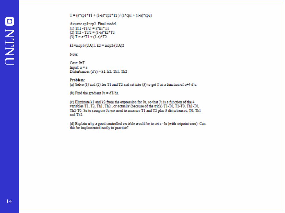
Parallel heat exchangersWhat should we control?
T0
m [kg/s]
Th2, UA2
T2
T1
T
α
1-α
• 1 Degree of freedom (u=split ®)• Objective: maximize J=T (= maximize total heat transfer Q)• What should we control?
- If active constraint : Control it! - Here: No active constraint.
• Control T? NO!
• Optimal: Control Ju=0
Th1, UA1

13
14

15
Controlling the gradient to zero, Ju=0
A. “Standard optimization (RTO)1. Estimate disturbances and present state
2. Use model to find optimal operation (usually numerically)
3. Implement optimal point. Alternatives: – Optimal inputs
– Setpoints cs to control layer (most common)
– Control computed gradient (which has setpoint=0)
Complex
C. Local loss method (local self-optimizing control)
1. Find linear expression for gradient, Ju = c= Hy
2. Control c to zero
Simple but assumesoptimal nominal point
Offline/ Online
1. Find expression for gradient (nonlinear analytic)
2. Eliminate unmeasured variables, Ju=f(y) (analytic)
3. Control gradient to zero:– Control layer adjust u until Ju = f(y)=0
Not generally possible,especially step 2
B. Analytic elimination (Jäschke method)
All these methods: Optimal only for assumed disturbances
Unconstrained degrees of freedom

16
Controlled variable, c = Hy
• y: all measured variables
• H: Nonsquare nc*ny matrix
– H selection matrix: Control single measurements
– H full matrix: Control measurement combinations
• nc=dim(c) = dim (u)
• Methods for finding H (c):1. Single variables: Intuition
2. Single variables: Large scaled gain
3. Combinations: Nullspace method (simple, but need ny=nu+nd)
4. Combinations: Exact local method (general)
Afterwards: Check using brute force evaluation
Unconstrained degrees of freedom

17
Linear measurement combinations, c = Hy
c=Hy is approximate gradient Ju
Two approaches
1.Nullspace method (HF=0): Simple but has limitations– Need many measurements if many disturbances (ny = nu + nd)– Does not handle measurement noise
2.Generalization: Exact local method+ Works for any measurement set y
+ Handles measurement error / noise
+
- Must assume that nominal point is optimal
Unconstrained degrees of freedom

18
Unconstrained variables
H
measurement noise
steady-statecontrol error
disturbance
controlled variable
/ selection
Ideal: c = Ju
In practise: c = H y
c
J
copt

19
WHAT ARE GOOD “SELF-OPTIMIZING” VARIABLES?
• Intuition: “Dominant variables” (Shinnar)
• Is there any systematic procedure?
A. Sensitive variables: “Max. gain rule” (Gain= Minimum singular value)
B. “Brute force” loss evaluation
C. Optimal linear combination of measurements, c = Hy
Unconstrained variables

20
«Brute force» analysis: What to control?
• Define optimal operation: Minimize cost function J
• Each candidate variable c:
With constant setpoints cs compute loss L for expected disturbances d and implementation errors n
• Select variable c with smallest loss

21
Constant setpoint policy:Loss for disturbances
Acceptable loss ) self-optimizing control
22
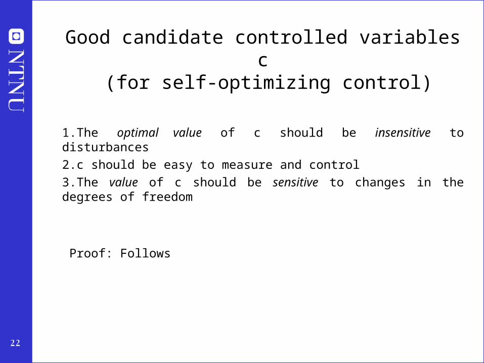
Good candidate controlled variables c (for self-optimizing control)
1.The optimal value of c should be insensitive to disturbances
2.c should be easy to measure and control
3.The value of c should be sensitive to changes in the degrees of freedom
Proof: Follows

23
Optimal operation
Cost J
Controlled variable cccoptopt
JJoptopt
Unconstrained optimum

24
Optimal operation
Cost J
Controlled variable cccoptopt
JJoptopt
Two problems:
• 1. Optimum moves because of disturbances d: copt(d)
• 2. Implementation error, c = copt + n
d
n
Unconstrained optimum

25
Candidate controlled variables c for self-optimizing control
Intuitive:
1. The optimal value of c should be insensitive to disturbances (avoid problem 1):
2. Optimum should be flat (avoid problem 2, implementation error).
Equivalently: Value of c should be sensitive to degrees of freedom u.
• “Want large gain”, |G|
• Or more generally: Maximize minimum singular value,
Unconstrained optimum
BADGoodGood

28
Optimizer
Controller thatadjusts u to keep
cm = cs
Plant
cs
cm=c+n
u
c
n
d
u
c
J
cs=copt
uopt
nu = G-1 n
) Want c sensitive to u (large gain G = dc/du)to get small variation in u (nu) when c varies (n)
Control sensitive variables
n

30
Maximum Gain Rule in words
In words, select controlled variables c for which
the gain G (= “controllable range”) is large compared to
its span (= sum of optimal variation and control error)
Select CVs that maximize (Gs)
Unconstrained variables
31
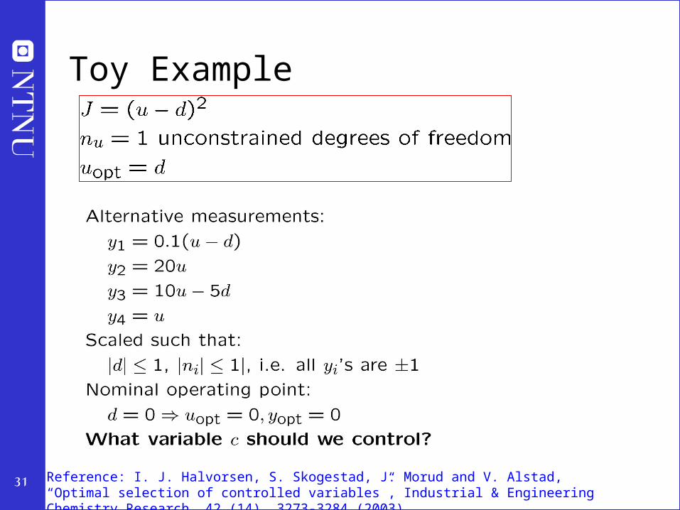
Toy Example
Reference: I. J. Halvorsen, S. Skogestad, J. Morud and V. Alstad, “Optimal selection of controlled variables”, Industrial & Engineering Chemistry Research, 42 (14), 3273-3284 (2003).
32
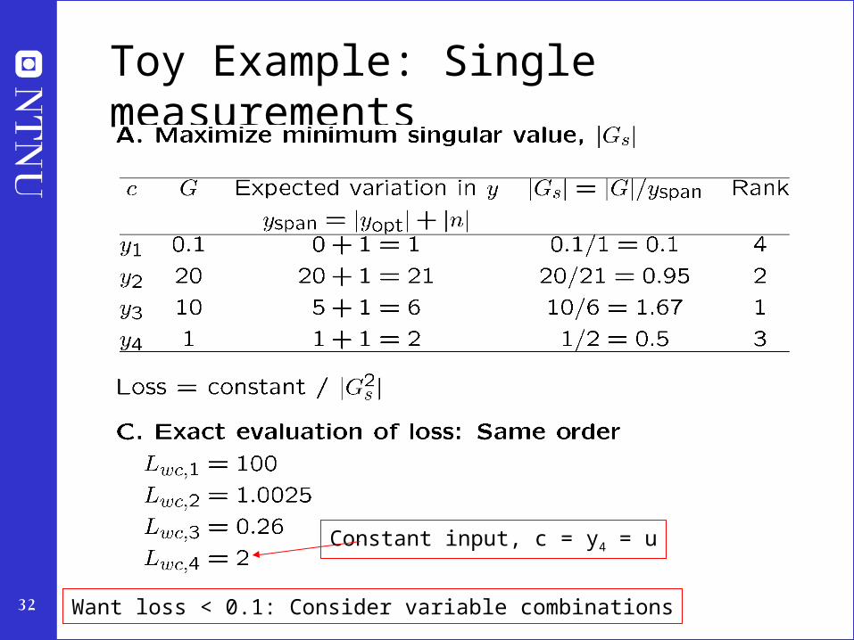
Toy Example: Single measurements
Want loss < 0.1: Consider variable combinations
Constant input, c = y4 = u

33
Summary: Procedure selection controlled variables
1. Define economics and operational constraints
2. Identify degrees of freedom and important disturbances
3. Optimize for various disturbances
4. Identify active constraints regions (off-line calculations)
For each active constraint region do step 5-6:
5. Identify “self-optimizing” controlled variables for remaining degrees of freedom
6. Identify switching policies between regions
34
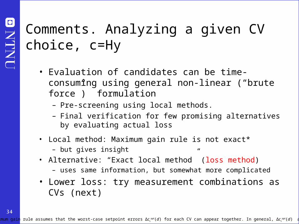
Comments. Analyzing a given CV choice, c=Hy
• Evaluation of candidates can be time-consuming using general non-linear (“brute force”) formulation– Pre-screening using local methods.
– Final verification for few promising alternatives by evaluating actual loss
• Local method: Maximum gain rule is not exact*– but gives insight
• Alternative: “Exact local method” (loss method)– uses same information, but somewhat more complicated
• Lower loss: try measurement combinations as CVs (next)
*The maximum gain rule assumes that the worst-case setpoint errors Δci,opt(d) for each CV can appear together. In general, Δci,
opt(d) are correlated.

35
Optimal measurement combination
•Candidate measurements (y): Include also inputs u
H
measurement noise
control error
disturbance
controlled variable
CV=Measurement combination

36
Nullspace method
No measurement noise (ny=0) CV=Measurement combination

37
Amazingly simple!
Sigurd is told how easy it is to find H
Proof nullspace methodBasis: Want optimal value of c to be independent of disturbances
• Find optimal solution as a function of d: uopt(d), yopt(d)
• Linearize this relationship: yopt = F d
– F – optimal sensitivity matrix
• Want: • To achieve this for all values of d:
• Always possible if
• Optimal when we disregard implementation error (n)
V. Alstad and S. Skogestad, ``Null Space Method for Selecting Optimal Measurement Combinations as Controlled Variables'', Ind.Eng.Chem.Res, 46 (3), 846-853 (2007).
No measurement noise (ny=0) CV=Measurement combination

38
Example. Nullspace Method for Marathon runner
u = power, d = slope [degrees]
y1 = hr [beat/min], y2 = v [m/s]
F = dyopt/dd = [0.25 -0.2]’
H = [h1 h2]]
HF = 0 -> h1 f1 + h2 f2 = 0.25 h1 – 0.2 h2 = 0
Choose h1 = 1 -> h2 = 0.25/0.2 = 1.25
Conclusion: c = hr + 1.25 v
Control c = constant -> hr increases when v decreases (OK uphill!)

39
Toy Example

40
Nullspace method (HF=0) gives Ju=0
• Proof. Appendix B in: Jäschke and Skogestad, ”NCO tracking and self-optimizing control in the context of real-time optimization”, Journal of Process Control, 1407-1416 (2011)
• .
Proof:

41
H/selection
Extension: ”Exact local method” (with measurement noise)
CV=Measurement combination
cm
Problem definition
(expected average with d normally distributed)

42
( , ) ( , )opt optL J u d J u d
Ref: Halvorsen et al. I&ECR, 2003
Kariwala et al. I&ECR, 2008
”Exact local method” (with measurement noise)
21/2 1( )yavg uu F
L J HG HYLoss with c=Hym=0 due to(i) Disturbances d(ii) Measurement noise ny
31( , ) ( , ) ( ) ( ) ( )
2T
opt u opt opt uu optJ u d J u d J u u u u J u u
1
[ ],d n
y yuu ud d
Y FW W
F G J J G
u
J
( )opt ou d
Loss
'd
Controlled variables,c yH
ydG
cs = constant +
+
+
+
+
- K
H
yG y
'yn
cm
u
dW nW
d
optu
CV=Measurement combination
44
'd
ydG
cs = constant +
+
+
+
+
- K
H
yG y
'yn
cm
u
dW nW
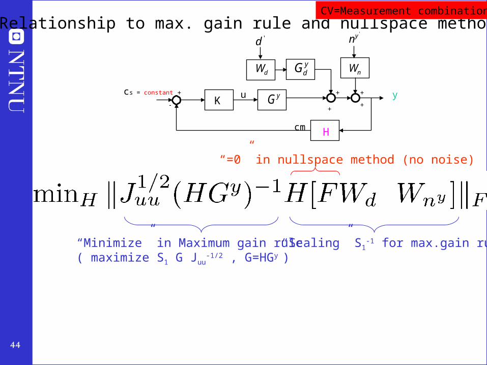
“Minimize” in Maximum gain rule( maximize S1 G Juu
-1/2 , G=HGy )
“Scaling” S1-1 for max.gain rule
“=0” in nullspace method (no noise)
Relationship to max. gain rule and nullspace methodCV=Measurement combination
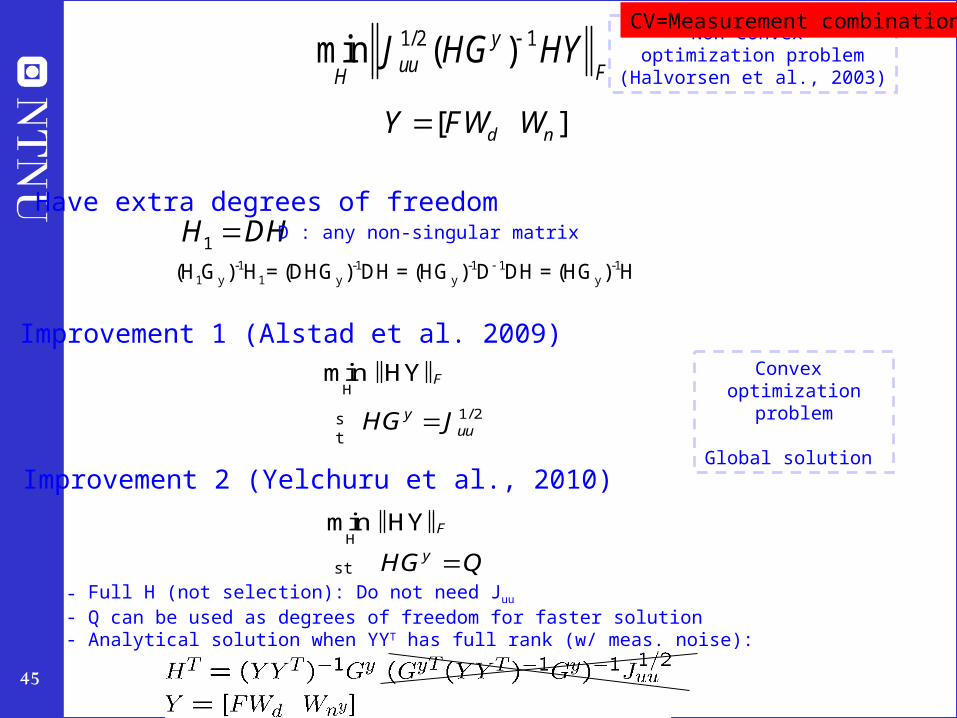
45
1/2 1min ( )yuu FH
J HG HY Non-convex optimization problem
(Halvorsen et al., 2003)
Hmin HY F
st 1/ 2yuuHG J
Improvement 1 (Alstad et al. 2009)
st yHG Q
Improvement 2 (Yelchuru et al., 2010)
Hmin HY F
-1 -1 -1 1 -11 y 1 y y y (H G ) H = (DHG ) DH = (HG ) D DH = (HG ) H
1H DH D : any non-singular matrix
Have extra degrees of freedom
[ ]d nY FW W
Convex optimization
problem
Global solution
- Full H (not selection): Do not need Juu
- Q can be used as degrees of freedom for faster solution- Analytical solution when YYT has full rank (w/ meas. noise):
1/2 1 1 1( ( ) ) ( )yT T y yT TuuH J G Y Y G G Y Y
CV=Measurement combination

46
Toy example...
47
Example: heat exchanger split

48
Example: CO2 refrigeration cycle
J = Ws (work supplied)DOF = u (valve opening, z)Main disturbances:
d1 = TH
d2 = TCs (setpoint) d3 = UAloss
What should we control?
pH

49
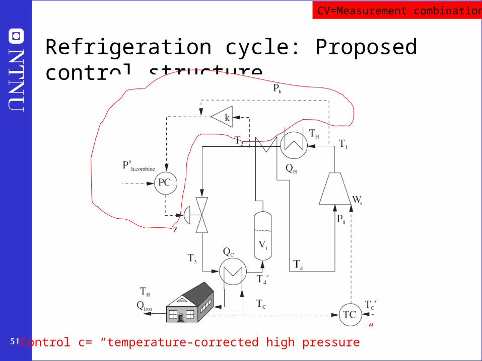
CO2 refrigeration cycle
Step 1. One (remaining) degree of freedom (u=z)
Step 2. Objective function. J = Ws (compressor work)
Step 3. Optimize operation for disturbances (d1=TC, d2=TH, d3=UA)• Optimum always unconstrained
Step 4. Implementation of optimal operation• No good single measurements (all give large losses):
– ph, Th, z, …
• Nullspace method: Need to combine nu+nd=1+3=4 measurements to have zero disturbance loss
• Simpler: Try combining two measurements. Exact local method:
– c = h1 ph + h2 Th = ph + k Th; k = -8.53 bar/K
• Nonlinear evaluation of loss: OK!

50
CO2 cycle: Maximum gain rule
51
Refrigeration cycle: Proposed control structure
Control c= “temperature-corrected high pressure”
CV=Measurement combination

52
Control structure design using self-optimizing control for economically optimal CO2 recovery*
Step S1. Objective function= J = energy cost + cost (tax) of released CO2 to air
Step S3 (Identify CVs). 1. Control the 4 equality constraints2. Identify 2 self-optimizing CVs. Use Exact Local method and select CV set with minimum loss.
4 equality and 2 inequality constraints:
1. stripper top pressure2. condenser temperature3. pump pressure of recycle amine4. cooler temperature
5. CO2 recovery ≥ 80%6. Reboiler duty < 1393 kW (nominal +20%)
4 levels without steady state effect: absorber 1,stripper 2,make up tank 1
*M. Panahi and S. Skogestad, ``Economically efficient operation of CO2 capturing process, part I: Self-optimizing procedure for selecting the best controlled variables'', Chemical Engineering and Processing, 50, 247-253 (2011).
Step S2. (a) 10 degrees of freedom: 8 valves + 2 pumps
Disturbances: flue gas flowrate, CO2 composition in flue gas + active constraints
(b) Optimization using Unisim steady-state simulator. Mode I = Region I (nominal feedrate): No inequality constraints active 2 unconstrained degrees of freedom =10-4-4
Case study

53
Exact local method* for finding2 self-optimizing CVs
The set with the minimum worst case loss is the best
21max. Loss= σ(M)
2-11/2 y
uu nyM=J (HG ) H [FW W ]d
y -1 yuu ud dF=G J J -G
opt.ΔyF=
Δd
* I.J. Halvorsen, S. Skogestad, J.C. Morud and V. Alstad, ‘Optimal selection of controlled variables’ Ind. Eng. Chem. Res., 42 (14), 3273-3284 (2003)
Juu and F, the optimal sensitivity of the measurements with respect to disturbances, are obtained numerically
54
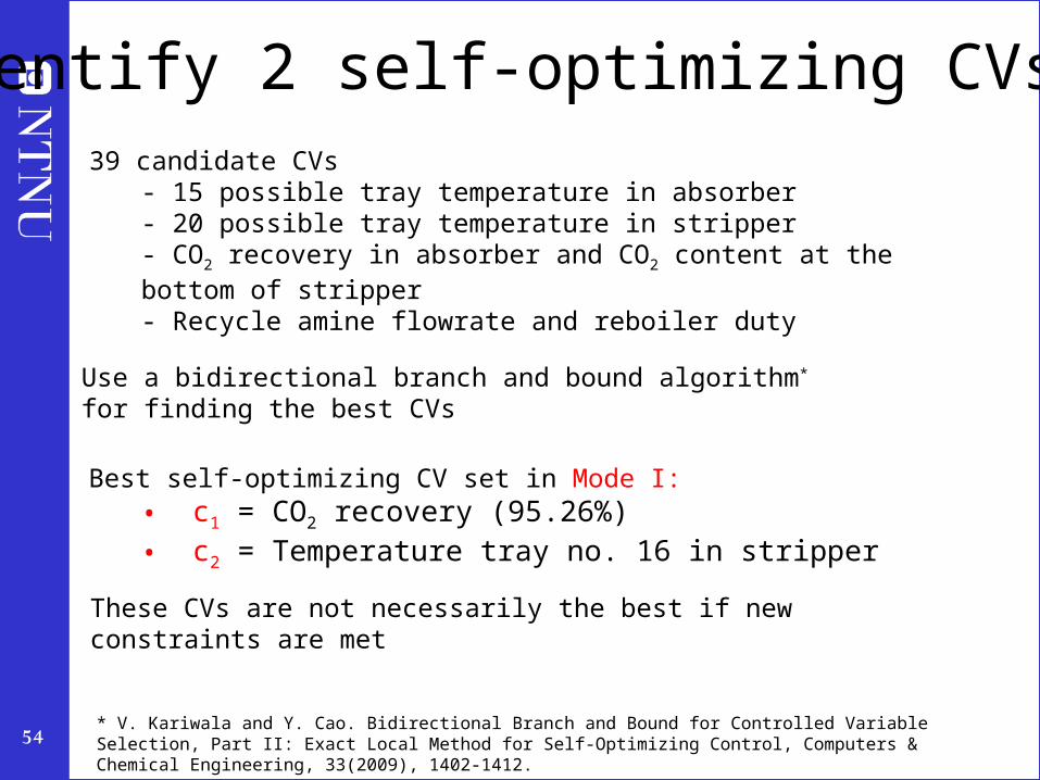
39 candidate CVs- 15 possible tray temperature in absorber- 20 possible tray temperature in stripper- CO2 recovery in absorber and CO2 content at the bottom of stripper- Recycle amine flowrate and reboiler duty
Best self-optimizing CV set in Mode I: • c1 = CO2 recovery (95.26%) • c2 = Temperature tray no. 16 in stripper
These CVs are not necessarily the best if new constraints are met
Use a bidirectional branch and bound algorithm* for finding the best CVs
* V. Kariwala and Y. Cao. Bidirectional Branch and Bound for Controlled Variable Selection, Part II: Exact Local Method for Self-Optimizing Control, Computers & Chemical Engineering, 33(2009), 1402-1412.
Identify 2 self-optimizing CVs

55
Proposed control structure with given
nominal flue gas flowrate (mode I)

56
Mode II: large feedrates of flue gas (+30%)
Feedrate flue gas (kmol/hr)
Self-optimizing CVs in region I Reboilerduty(kW)
Cost(USD/ton)
CO2 recovery
%
Temperaturetray no. 16
°C
Optimal nominal point 219.3 95.26 106.9 1161 2.49
+5% feedrate 230.3 95.26 106.9 1222 2.49
+10% feedrate 241.2 95.26 106.9 1279 2.49
+15% feedrate 252.2 95.26 106.9 1339 2.49
+19.38%, when reboiler duty saturates
261.8 95.26 106.9 1393(+20%)
2.50
+30% feedrate (reoptimized)
285.1 91.60 103.3 1393 2.65
Saturation of reboiler duty; one unconstrained degree of freedom left
Use Maximum gain rule to find the best CV among 37 candidates :
• Temp. on tray no. 13 in the stripper: largest scaled gain, but tray 16 also OK
region I
region II
max

57
Proposed control structure with large flue gas flowrate (mode II = region II)
max

58
Conditions for switching between regions of active constraints (“supervisory control”)
• Within each region of active constraints it is optimal to 1. Control active constraints at ca = c,a, constraint
2. Control self-optimizing variables at cso = c,so, optimal
• Define in each region i:
• Keep track of ci (active constraints and “self-optimizing” variables) in all regions i
• Switch to region i when element in ci changes sign
59
Example – switching policies CO2 plant(”supervisory control”)
• Assume operating in region I (unconstrained) – with CV=CO2-recovery=95.26%
• When reach maximum Q: Switch to Q=Qmax (Region II) (obvious)– CO2-recovery will then drop below 95.26%
• When CO2-recovery exceeds 95.26%: Switch back to region I !!!

61
Conclusion optimal operation
ALWAYS:
1. Control active constraints and control them tightly!!– Good times: Maximize throughput -> tight control of bottleneck
2. Identify “self-optimizing” CVs for remaining unconstrained degrees of freedom
• Use offline analysis to find expected operating regions and prepare control system for this!
– One control policy when prices are low (nominal, unconstrained optimum)
– Another when prices are high (constrained optimum = bottleneck)
ONLY if necessary: consider RTO on top of this

62
Sigurd’s rules for CV selection
1. Always control active constraints! (almost always)
2. Purity constraint on expensive product always active (no overpurification):
(a) "Avoid product give away" (e.g., sell water as expensive product)
(b) Save energy (costs energy to overpurify)
3. Unconstrained optimum: NEVER try to control a variable that reaches max or min at the optimum
–In particular, never try to control directly the cost J
–- Assume we want to minimize J (e.g., J = V = energy) - and we make the stupid choice os selecting CV = V = J - Then setting J < Jmin: Gives infeasible operation (cannot meet constraints) - and setting J > Jmin: Forces us to be nonoptimal (which may require strange operation; see Exercise 3 on evaporators)