lable at ScienceDirect

Journal of Power Sources 252 (2014) 214e228

Contents lists avai

Journal of Power Sources

journal homepage: www.elsevier .com/locate/ jpowsour

Numerical simulation of thermal behavior of lithium-ion secondarybatteries using the enhanced single particle model

Naoki Baba a,*, Hiroaki Yoshida a, Makoto Nagaoka a, Chikaaki Okuda b,Shigehiro Kawauchi b

a Thermodynamic System Research Div., Toyota Central R&D Labs., Inc., Nagakute, Aichi 480-1192, Japanb Energy Creation & Storage Div., Toyota Central R&D Labs., Inc., Nagakute, Aichi 480-1192, Japan

h i g h l i g h t s

� We propose an enhanced single particle (ESP) model for lithium-ion batteries.� The ESP model accounts for the solution phase limitation.� The ESP model is available for the high rate chargeedischarge analysis.� We report the two-way electrochemical-thermal coupled simulation method.� Temperature estimates during the chargeedischarge cycle are calculated accurately.

a r t i c l e i n f o

Article history:Received 11 October 2013Received in revised form27 November 2013Accepted 29 November 2013Available online 10 December 2013

Keywords:Lithium-ion batteryThermal behaviorSimulationBattery modelingSingle particle modelTwo-way coupling

* Corresponding author. Tel.: þ81 561 71 7064; faxE-mail address: baba-n@mosk.tytlabs.co.jp (N. Bab

0378-7753/$ e see front matter � 2013 Elsevier B.V.http://dx.doi.org/10.1016/j.jpowsour.2013.11.111

a b s t r a c t

To understand the thermal behavior of lithium-ion secondary batteries, distributed information relatedto local heat generation across the entire electrode plane, which is caused by the electrochemical re-action that results from lithium-ion intercalation or deintercalation, is required. To accomplish this, wefirst developed an enhanced single particle (ESP) model for lithium-ion batteries that provides a costeffective, timely, and accurate method for estimating the local heat generation rates without excessivecomputation costs. This model accounts for all the physical processes, including the solution phaselimitation. Next, a two-way electrochemical-thermal coupled simulation method was established. In thismethod, the three dimensional (3D) thermal solver is coupled with the quasi-3D porous electrode solverthat is applied to the unrolled plane of spirally wound electrodes, which allows both thermal andelectrochemical behaviors to be reproduced simultaneously at every computational time-step. The quasi-3D porous electrode solver implements the ESP model.

This two-way coupled simulation method was applied to a thermal behavior analysis of 18650-typelithium-ion cells where it was found that temperature estimates of the electrode interior and on thecell can wall obtained via the ESP model were in good agreement with actual experimentalmeasurements.

� 2013 Elsevier B.V. All rights reserved.

1. Introduction

Lithium-ion batteries are attractive power sources for hybridelectric vehicles (HEVs) and electric vehicles (EVs) because theyoffer high cell voltages and energy densities. As a result, significantamounts of research have been focused on improving the powerdensity, energy density, and life cycle performance of such batte-ries. However, because one of the primary issues in designing

: þ81 561 63 6920.a).

All rights reserved.

lithium-ion batteries is ensuring safety, ceaseless efforts have beenexpended towards overcoming thermal stability problems.

When evaluating thermal stability in the battery design phase,numerical simulation techniques provide useful information that isdifficult or impossible to obtain experimentally. As a result, therehave been numerous previous reports on thermal modeling oflithium-ion batteries over a wide range of exposed conditions.Many such reports go beyond normal use [1e11], with somefocusing specifically on thermal abuse [12,13].

For example, Pals and Newman performed one-dimensional(1D) thermal modeling experiments to calculate temperature pro-files in cell stacks [5,6]. This work was based on the 1Dmacroscopicmodel developed by Doyle and Newman [14] with the addition of a

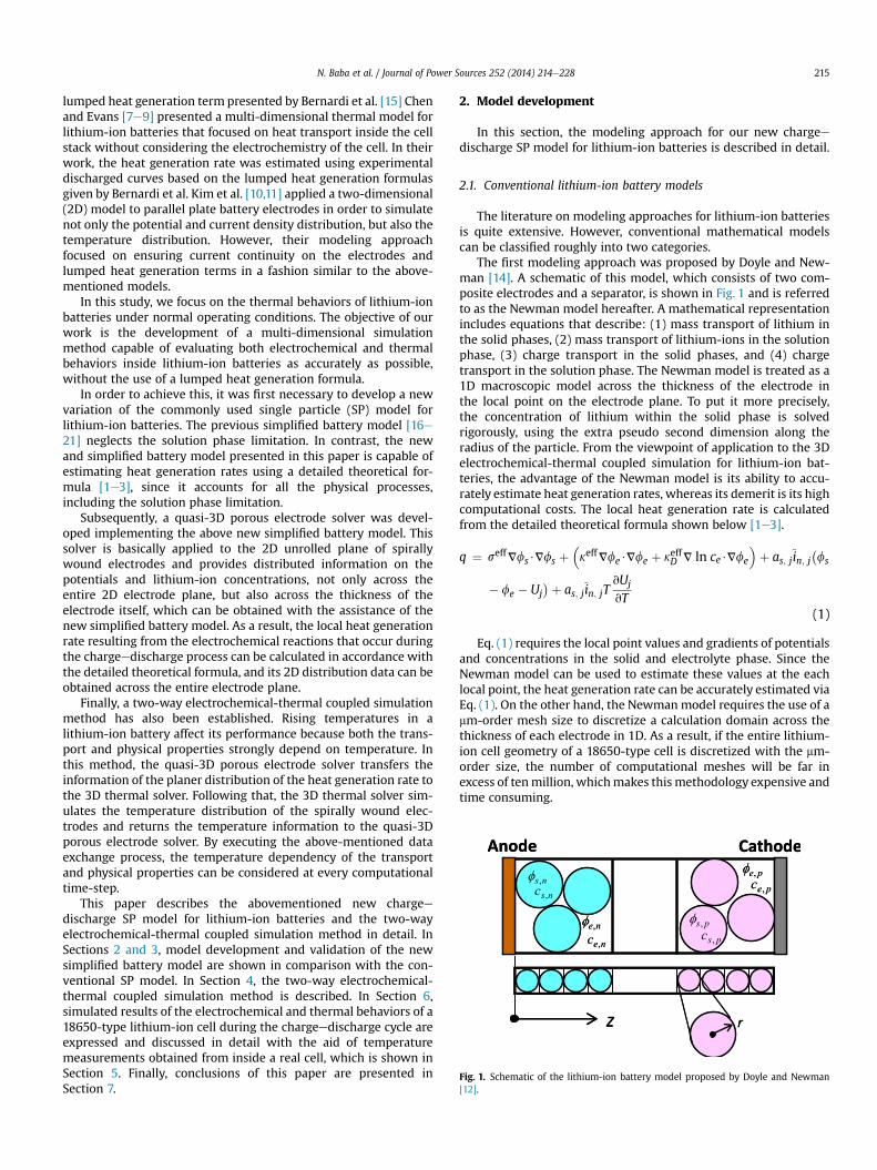
Fig. 1. Schematic of the lithium-ion battery model proposed by Doyle and Newman[12].

N. Baba et al. / Journal of Power Sources 252 (2014) 214e228 215

lumped heat generation term presented by Bernardi et al. [15] Chenand Evans [7e9] presented a multi-dimensional thermal model forlithium-ion batteries that focused on heat transport inside the cellstack without considering the electrochemistry of the cell. In theirwork, the heat generation rate was estimated using experimentaldischarged curves based on the lumped heat generation formulasgiven by Bernardi et al. Kim et al. [10,11] applied a two-dimensional(2D) model to parallel plate battery electrodes in order to simulatenot only the potential and current density distribution, but also thetemperature distribution. However, their modeling approachfocused on ensuring current continuity on the electrodes andlumped heat generation terms in a fashion similar to the above-mentioned models.

In this study, we focus on the thermal behaviors of lithium-ionbatteries under normal operating conditions. The objective of ourwork is the development of a multi-dimensional simulationmethod capable of evaluating both electrochemical and thermalbehaviors inside lithium-ion batteries as accurately as possible,without the use of a lumped heat generation formula.

In order to achieve this, it was first necessary to develop a newvariation of the commonly used single particle (SP) model forlithium-ion batteries. The previous simplified battery model [16e21] neglects the solution phase limitation. In contrast, the newand simplified battery model presented in this paper is capable ofestimating heat generation rates using a detailed theoretical for-mula [1e3], since it accounts for all the physical processes,including the solution phase limitation.

Subsequently, a quasi-3D porous electrode solver was devel-oped implementing the above new simplified battery model. Thissolver is basically applied to the 2D unrolled plane of spirallywound electrodes and provides distributed information on thepotentials and lithium-ion concentrations, not only across theentire 2D electrode plane, but also across the thickness of theelectrode itself, which can be obtained with the assistance of thenew simplified battery model. As a result, the local heat generationrate resulting from the electrochemical reactions that occur duringthe chargeedischarge process can be calculated in accordance withthe detailed theoretical formula, and its 2D distribution data can beobtained across the entire electrode plane.

Finally, a two-way electrochemical-thermal coupled simulationmethod has also been established. Rising temperatures in alithium-ion battery affect its performance because both the trans-port and physical properties strongly depend on temperature. Inthis method, the quasi-3D porous electrode solver transfers theinformation of the planer distribution of the heat generation rate tothe 3D thermal solver. Following that, the 3D thermal solver sim-ulates the temperature distribution of the spirally wound elec-trodes and returns the temperature information to the quasi-3Dporous electrode solver. By executing the above-mentioned dataexchange process, the temperature dependency of the transportand physical properties can be considered at every computationaltime-step.

This paper describes the abovementioned new chargeedischarge SP model for lithium-ion batteries and the two-wayelectrochemical-thermal coupled simulation method in detail. InSections 2 and 3, model development and validation of the newsimplified battery model are shown in comparison with the con-ventional SP model. In Section 4, the two-way electrochemical-thermal coupled simulation method is described. In Section 6,simulated results of the electrochemical and thermal behaviors of a18650-type lithium-ion cell during the chargeedischarge cycle areexpressed and discussed in detail with the aid of temperaturemeasurements obtained from inside a real cell, which is shown inSection 5. Finally, conclusions of this paper are presented inSection 7.

2. Model development

In this section, the modeling approach for our new chargeedischarge SP model for lithium-ion batteries is described in detail.

2.1. Conventional lithium-ion battery models

The literature on modeling approaches for lithium-ion batteriesis quite extensive. However, conventional mathematical modelscan be classified roughly into two categories.

The first modeling approach was proposed by Doyle and New-man [14]. A schematic of this model, which consists of two com-posite electrodes and a separator, is shown in Fig. 1 and is referredto as the Newman model hereafter. A mathematical representationincludes equations that describe: (1) mass transport of lithium inthe solid phases, (2) mass transport of lithium-ions in the solutionphase, (3) charge transport in the solid phases, and (4) chargetransport in the solution phase. The Newman model is treated as a1D macroscopic model across the thickness of the electrode inthe local point on the electrode plane. To put it more precisely,the concentration of lithium within the solid phase is solvedrigorously, using the extra pseudo second dimension along theradius of the particle. From the viewpoint of application to the 3Delectrochemical-thermal coupled simulation for lithium-ion bat-teries, the advantage of the Newman model is its ability to accu-rately estimate heat generation rates, whereas its demerit is its highcomputational costs. The local heat generation rate is calculatedfrom the detailed theoretical formula shown below [1e3].

q ¼ seffVfs$Vfs þ�keffVfe$Vfe þ keffD V ln ce$Vfe

�þ as; jin; j

�fs

� fe � Uj�þ as; jin; jT

vUj

vT(1)

Eq. (1) requires the local point values and gradients of potentialsand concentrations in the solid and electrolyte phase. Since theNewman model can be used to estimate these values at the eachlocal point, the heat generation rate can be accurately estimated viaEq. (1). On the other hand, the Newmanmodel requires the use of amm-order mesh size to discretize a calculation domain across thethickness of each electrode in 1D. As a result, if the entire lithium-ion cell geometry of a 18650-type cell is discretized with the mm-order size, the number of computational meshes will be far inexcess of tenmillion, whichmakes this methodology expensive andtime consuming.

Fig. 3. Schematic of the ESP model. In this model, each of negative and positiveelectrodes is represented by a single spherical particle in the electrolyte phase.

N. Baba et al. / Journal of Power Sources 252 (2014) 214e228216

The second modeling approach is the SP model [16e21]. Aschematic of this model is shown in Fig. 2. In this model, eachelectrode is represented by a single spherical particle. Whenconsidering the 3D electrochemical-thermal coupled simulation oflithium-ion batteries, it is important to reflect on the advantagesand drawbacks of the SP model. The advantages of the SP modelinclude its simplicity and reduced computation time requirements.This model is orders of magnitude faster than the Newman model.However, a significant drawback of the SP model is that it assumesthat the electrolyte phase diffusion limitations are ignored. Hence,potentials in the electrolyte phase are set to zero, and concentra-tions in the electrolyte phase are set to a constant value. This ren-ders estimations of the heat generation rate via Eq. (1) inadequate.Furthermore, even if the heat generation rate is estimated using thelumped formula presented by Bernardi et al. [15], the resultingestimated values seem to have less accuracy.

2.2. Description of new SP model

In the above discussion, the advantages and drawbacks of con-ventional lithium-ion battery models were classified. In the presentpaper, from the viewpoint of application to the 3D electrochemical-thermal coupled simulation, we propose a new lumped model forlithium-ion batteries.

This model combines advantages of both the Newman and SPmodels. However, to be successful, the new lumped model mustprovide the following advantages:

(a) Calculation costs equivalent to that of the SP model(b) Heat release rate estimation accuracy at same level as the

Newman model

The development concept of a new lumped model is based onthe SP model with specific consideration paid to the electrolytephase diffusion limitations. Fig. 3 shows a schematic of a newlumped model, which is referred to hereafter as the enhancedsingle particle (ESP) model. In the ESP model, each electrode isrepresented by a single spherical particle along with its electrolytephase. The potential and lithium concentration in the solid phaseare calculated in the same way as with the conventional SP model.Additionally, the potential and lithium-ion concentration in theelectrolyte phase are set at the representative position in the eachelectrode.

The most important advancement over the SP model at thispoint is that these physical quantities are approximated by para-bolic profiles within each electrode. As described in Eq. (1), accurateheat release rate estimates require the point values and gradients ofthese physical quantities. These point values and gradients arecalculated from approximated parabolic profiles, which makes itpossible for the ESP model to calculate the heat release rate.Furthermore, the potentials and lithium-ion concentrations at in-terfaces between the negative and the separator, or between thepositive and the separator, are implicitly considered in the ESP

Fig. 2. Schematic of the single particle (SP) model. This model assumes that theelectrolyte phase diffusion limitations are ignored.

model. Mass transport and charge transport between both elec-trodes in the electrolyte phase, which satisfies the mass and chargeconservation, are estimated using these boundary values.

2.3. Model equations

2.3.1. Calculation procedure of concentrationsFig. 4 describes the procedure for calculating ESP model con-

centrations in detail.Fick’s second law usually describes the lithium transport in the

solid phase, with the following boundary conditions set for aspherical particle:

vcsvt

¼ Ds

"v2csvr2

þ 2rvcsvr

#(2)

�Dsvcsvr

¼ 0 at r ¼ 0 (3)

�Dsvcsvr

¼ inF

at r ¼ rs (4)

In the conventional SP model, the diffusion length method [22]is introduced to simplify the diffusion equation. By assuming aparabolic concentration profile in the diffusion layer and using the

Fig. 4. Calculation procedure of the concentration field of the ESP model.

Fig. 5. Calculation procedure of the potential field of the ESP model.

N. Baba et al. / Journal of Power Sources 252 (2014) 214e228 217

volume average technique, the solutions for Eqs. (2)e(4) can beapproximated with a set of differential and algebraic equations:

dcs;jdt

þ 15Ds; j

r2s; j

�cs; j � cse; j

� ¼ 0 (5)

�Ds; j

�cse; j � cs; j

�lse; j

¼jLij

as; jF(6)

where lse,j is the diffusion length and takes the value of rs,j/5 forspherical particles. In view of the need to reduce computationalcosts, the diffusion lengthmethod is implemented to the ESPmodelin the same way.

The diffusion limitations in the electrolyte phase are alsoconsidered in the ESP model. The representative lithium-ion con-centrations of electrolyte in each electrode region are defined byusing the volume average technique as follows:

ce; n ¼ 1Ln

ZLn0

ce; ndzn (7)

ce; p ¼ 1Lp

ZLp0

ce; pdzp (8)

In the ESPmodel, a parabolic concentration profile is assumed ineach region. Therefore, the positions corresponding to the repre-sentative concentrations are

z*n; e ¼ 1ffiffiffi3

p $Ln (9)

z*p; e ¼�1� 1ffiffiffi

3p�$Lp (10)

where the extra pseudo coordinates zn and zp are defined as shownin Fig. 4.

In addition, as Fig. 4 also shows, the concentrations on thenegative/separator interface and the separator/positive interfaceare implicitly defined as cif, 1 and cif, 2, respectively. The interfacialbalances of lithium-ion flux yield are

�Deffe; n

cif ; 1 � ce; ndn

¼ �Deffe; sep

cif ; 2 � cif ; 1Lsep

(11)

�Deffe; sep

cif ; 2 � cif ;1Lsep

¼ �Deffe; p

ce; p � cif ; 2dp

(12)

where dn and dp represent the diffusion length in each regionwhichare expressed as [22]

dn ¼ Ln3

and dp ¼ Lp3

(13)

Solving Eqs. (11) and (12) gives the interfacial concentrations as

cif ; 1 ¼ an þ u

an þ uþ gp$ce; n þ

gpan þ uþ gp

$ce; p (14)

cif ; 2 ¼ anan þ uþ gp

$ce; n þuþ gp

an þ uþ gp$ce; p (15)

an ¼ Deffe; n

dn; bsep ¼ Deff

e; sep

Lsep; gp ¼ Deff

e; p

dpand u ¼ gp$an

bsep

(16)

The equations for calculating the time evolution of the volumeaveraged lithium-ion concentration in the electrolyte phase arederived as shown below. As for the negative, conservation oflithium-ion [14] in the electrolyte yields

εe; nvce; nvt

¼ Deffe; n

v2ce; nvz2n

þ 1� t�þ

FjLin (17)

As shown in Fig. 4, the electrolyte phase concentration is rep-resented by a parabolic profile:

ce; n ¼ a$z2n þ b$zn þ c (18)

where the three coefficients, a, b and c can be determined by thefollowing boundary conditions and Eq. (7).

vce; nvzn

¼ 0 at zn ¼ 0 (19)

ce; n ¼ cif ; 1 at zn ¼ Ln (20)

Application of volume averaging to Eq. (17) and substitution ofEq. (18) results in

εe; ndce; ndt

¼ Deffe; n$ð2aÞ þ

1� t�þ

FjLin (21)

Substituting the coefficient a into Eq. (21) yields

εe; ndce; ndt

¼ An$ce; n þ Bn$ce; p þ1� t

�þ

FjLin (22)

where the coefficients An and Bn are given by

An ¼ � 1Ln$

gp$an

an þ uþ gp(23)

Bn ¼ 1Ln$

gp$an

an þ uþ gp(24)

As for the positive, the same procedure mentioned above alsoyields the equation for calculating the time evolution of the volumeaveraged lithium-ion concentration in the electrolyte phase:

N. Baba et al. / Journal of Power Sources 252 (2014) 214e228218

εe; pdce; p ¼ Ap$ce; n þ Bp$ce; p þ

1� t�þjLip (25)

dt F

where the coefficients Ap and Bp are given by

Ap ¼ 1Lp$

gp$an

an þ uþ gp(26)

Bp ¼ � 1Lp$

gp$an

an þ uþ gp(27)

Currently, in the ESP model, Eqs. (5), (6), (22) and (25) arespecified in order to solve the mass transport of the system.

2.3.2. Calculation procedure of potentialsWith the assistance of Fig. 5, the calculation procedure of po-

tentials of the ESP model is described in detail. In analogy with thecalculation procedure of concentrations, the potentials on thenegative/separator interface and the separator/positive interfaceare implicitly defined as ɸif, 1 and ɸif, 2, respectively.

The boundary conditions for the solid phase potential ɸs,n in thenegative electrode are described below. On the copper currentcollector/composite negative electrode interface, ɸs,n is arbitrarilyset to zero, while on the same interface, the solid phase currentdensity is equated to the applied current density, namely

fs; n ¼ 0 at zn ¼ 0 (28)

�seffnvfs; n

vzn¼ Iapp at zn ¼ 0 (29)

On the negative/separator interface, the charge flux in the solidphase is equated to zero.

vfs; n

vzn¼ 0 at zn ¼ Ln (30)

Applying a parabolic profile for ɸs,n, satisfaction of the aboveboundary conditions results in

fs; n ¼ 12Ln

$Iappseffn

$z2n �Iappseffn

$zn (31)

The representative potential in the negative solid phase isdefined by using the volume average technique.

fs; n ¼ 1Ln

ZLn0

fs; ndzn (32)

Substituting Eq. (31) into Eq. (32) gives

fs; n ¼ �13$Lnseffn

$Iapp (33)

This is equal to the point value that is calculated in the profile,Eq. (31), at

z*n; s ¼�1� 1ffiffiffi

3p�$Ln (34)

The calculation procedure of the other potentials (fe; n, ɸif, 1, ɸif, 2,fe; p,fs; p) are described sequentially below.

Because Eq. (33) gives the solid phase potential, fs; n, therepresentative potential in the negative electrolyte region, fe; n, isdetermined by the following ButlereVolmer equation, namely

Iapp ¼ as; ni0; n expaa; nF hn

� �� exp �ac; nF hn

� � (35)

Ln RT RT

where the surface overpotential, hn, is defined to be

hn ¼ fs; n � fe; n � Un � in; n$Rf ; n (36)

Conservation of charge in the electrolyte phase results in [14]

V$�keffj Vfe; j

�þ V$

�keffD; jV ln ce; j

�þ jLij ¼ 0 (37)

From Eq. (37), the charge flux on the negative/separator inter-face is equated to the applied current density:

�keffnvfe; n

vzn

����zn¼Ln

� keffD; n

vce; nvzn

���zn¼Ln

cif ; 1¼ Iapp (38)

Since the second term of the left-hand side is estimated usingEqs. (14) and (18), the potential gradient on the negative/separatorinterface (the first term) is obtained from Eq. (38). Next, a parabolicprofile is assumed for the electrolyte potential across the thicknessof the negative electrode. This parabolic profile must meet thefollowing three conditions:

vfe; n

vzn¼ at zn ¼ 0 (39)

vfe; n

vzn¼ sif ; 1 at zn ¼ Ln (40)

fe; n ¼ 1Ln

ZLn0

fe; ndzn (41)

where sif, 1 is the electrolyte potential gradient on the negative/separator interface, which is estimated from Eq. (38). Using Eqs.(39)e(41), the potential profile in the negative electrolyte region isfound to be determined by

fe; n ¼ sif ; 12Ln

$z2n þ fe; n �sif ; 16

$Ln (42)

According to Eq. (42), the interfacial potential ɸif, 1 is readilyfound to be expressed by

fif ; 1 ¼ sif ; 13

$Ln þ fe; n (43)

Taking into account the continuity of the charge flux in theelectrolyte phase, the charge transport in the separator leads to

fif ; 2 ¼ fif ; 1 �1

keffsep

Iapp$Lsep þ keffD;sep$ln

cif ; 2cif ; 1

!(44)

where the interfacial concentrations, cif, 1 and cif, 2, can be estimatedby Eqs. (14) and (15).

A similar calculation procedure, which is mentioned above,derives the parabolic profile for the positive electrolyte potential.The charge flux on the positive/separator interface is equated to theapplied current density:

�keffpvfe; p

vzp

����zp¼0

� keffD; p

vce; p

vz

���zp¼0

cif ; 2¼ Iapp (45)

The second term on the left is estimated by using Eq. (15) andthe parabolic profile of ce, p. This allows the potential gradient on

N. Baba et al. / Journal of Power Sources 252 (2014) 214e228 219

the separator/positive interface in the first term to be estimated. Aparabolic profile is assumed for the electrolyte potential across thethickness of the positive electrode. This parabolic profile mustsatisfy the following conditions:

fe; p ¼ fif ; 2 at zp ¼ 0 (46)

vfe; p

vzp¼ sif ; 2 at zp ¼ 0 (47)

vfe; p

vzp¼ 0 at zp ¼ Lp (48)

where sif, 2 is the electrolyte potential gradient on the separator/positive interface, which is estimated from Eq. (45). Using Eqs.(46)e(48), the potential profile in the positive electrolyte phase isfound to be expressed by

fe; p ¼ �sif ; 22Lp

$z2p þ sif ; 2$zp þ fif ; 2 (49)

The representative potential in the positive electrolyte isdefined to be

fe; p ¼ 1Lp

ZLp0

fe; pdzp ¼ sif ; 23

Lp þ fif ; 2 (50)

This is equal to the point value that is calculated in the profile ofEq. (49) at z*p; e (Eq. (10)).

Finally, let us turn to the positive solid phase potential. As Eq.(50) gives the electrolyte phase potential, the representative po-tential in the positive solid phase, fs; p, is estimated by thefollowing ButlereVolmer equation, namely

�IappLp

¼ as; pi0; p

exp

�aa; pFRT

hp

�� exp

�� ac; pF

RThp

�(51)

where the surface overpotential, hp, is defined to be

hp ¼ fs; p � fe; p � Up � in; p$Rf ;p (52)

Just as in the case of the solid phase potential in the negativeelectrode, ɸs,n, a parabolic profile is assumed and must meet thefollowing conditions to determine the three coefficients.

vfs; p

vzp¼ 0 at zp ¼ 0 (53)

�seffs; pvfs; p

vzp¼ Iapp at zp ¼ Lp (54)

fs; p ¼ 1Lp

ZLp0

fs; pdzp (55)

Satisfaction of above conditions results in

fs; p ¼ � 12Lp

$Iappseffs; p

$z2p þLp6$Iappseffs; p

þ fs; p (56)

The representative value, fs;p, is obtained in the profile, Eq. (56),at

z*p; s ¼ 1ffiffiffi3

p $Lp (57)

2.3.3. Summary of model equationsModel equations of the ESPmodel are now specified completely.

The final equations are summarized in Table 1. Time evolutions ofunknowns are calculated by using the set of equations for volumeaveraging values.

Here, the relationship between the conventional SP model andthe ESP model is worth a passing mention. The conventional SPmodel assumes that the diffusion limitations in the electrolytephase are negligible. This assumption leads to omitting all equa-tions in the electrolyte phase from the ESP model presented in thispaper. The conservation of charge in the negative solid phase isgiven by

seffnv2fs; n

vz2n� jLin ¼ 0 (58)

Applying Eq. (31) to Eq. (58) yields

IappLn

� jLin ¼ 0 (59)

The above equation is also used in the conventional SP model.Note that the ESP model that neglects the electrolyte phase diffu-sion limitations reduces to the conventional SP model.

2.3.4. Estimation of heat generation rateThe heat generation rate during the chargeedischarge process,

which is Eq. (1) as revised for the ESP model, is expressed by

q ¼X

j¼n; p

�seffj Vfs; j$Vfs; j

�þ

Xj¼n; sep; p

�keffj Vfe; j$Vfe; j

þ keffD; jV ln ce; j$Vfe; j

�þX

j¼n; p

as; jin; j�fs; j � fe; j � Uj

�

þX

j¼n; p

as; jin; jTvUj

vT

(60)

The first term results from the ohmic heat in the solid phase,while the second term arises from the ohmic heat in the electrolytephase. The summation of the last two terms accounts for irre-versible and reversible heats associated with charge transfer at thesolid/electrolyte interfaces. The third term represents the potentialdeviation from the equilibrium potential (irreversible heat). Thefourth term arises from the entropic effect (reversible heat).

From Eq. (60), it is clear that the estimation of ohmic heats in thesolid and electrolyte phases needs the information about the gra-dients of the unknowns. The ESP model includes the profile infor-mation of concentrations and potentials across the thickness of theelectrode as standard features, as shown in Table 1. The gradients ofconcentrations and potentials in the solid phase are estimated ineach parabolic profile at the positions of z*n; s (Eq. (34), for thenegative) and z*p; s (Eq. (57), for the positive). Additionally, thegradients in the electrolyte phase are estimated in each parabolicprofile at the positions of z*n; e (Eq. (9), for the negative) and z*p; e (Eq.(10), for the positive). As for estimation of irreversible and revers-ible heats, volume averaging values are used.

3. Model validation

3.1. Comparison with Newman model accuracy

First we examined the cell potential during galvanostaticdischarge at various current densities for the cell described inRef. 23. This cell consists of a carbon negative electrode (LixC6), a

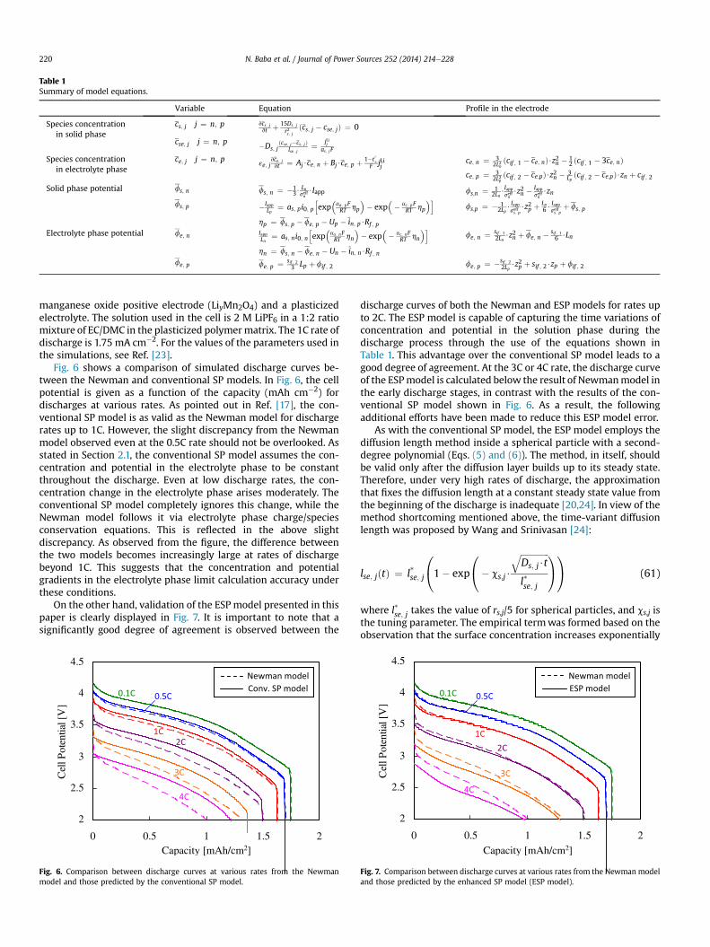
Table 1Summary of model equations.

Variable Equation Profile in the electrode

Species concentrationin solid phase

cs; j j ¼ n; p vcs; j

vt þ 15Ds; j

r2s; jðcs; j � cse; jÞ ¼ 0

cse; j j ¼ n; p �Ds; jðcse; j�cs; jÞ

lse; j¼ jLij

as; jF

Species concentrationin electrolyte phase

ce; j j ¼ n; pεe; j

vce; j

vt ¼ Aj$ce; n þ Bj$ce; p þ 1�t�þ

F jLijce; n ¼ 3

2L2nðcif ; 1 � ce; nÞ$z2n � 1

2 ðcif ; 1 � 3ce; nÞce; p ¼ 3

2L2pðcif ; 2 � ce;pÞ$z2n � 3

Lpðcif ; 2 � ce;pÞ$zn þ cif ; 2

Solid phase potential fs; n fs; n ¼ �13$

Lnseffn$Iapp fs;n ¼ 1

2Ln$Iappseffn$z2n � Iapp

seffn$zn

fs; p �IappLp

¼ as; pi0; phexp

�aa; pFRT hp

�� exp

�� ac; pF

RT hp

�ihp ¼ fs; p � fe; p � Up � in; p$Rf ; p

fs;p ¼ � 12Lp

$Iappseffs; p$z2p þ Lp

6 $Iappseffs; p

þ fs; p

Electrolyte phase potential fe; n IappLn

¼ as; ni0; nhexp

�aa; nFRT hn

�� exp

�� ac; nF

RT hn

�ihn ¼ fs; n � fe; n � Un � in; n$Rf ; n

fe; n ¼ sif ; 1

2Ln$z2n þ fe; n � sif ; 1

6 $Ln

fe; p fe; p ¼ sif ; 2

3 Lp þ fif ; 2 fe; p ¼ �sif ; 2

2Lp$z2p þ sif ; 2$zp þ fif ; 2

N. Baba et al. / Journal of Power Sources 252 (2014) 214e228220

manganese oxide positive electrode (LiyMn2O4) and a plasticizedelectrolyte. The solution used in the cell is 2 M LiPF6 in a 1:2 ratiomixture of EC/DMC in the plasticized polymermatrix. The 1C rate ofdischarge is 1.75 mA cm�2. For the values of the parameters used inthe simulations, see Ref. [23].

Fig. 6 shows a comparison of simulated discharge curves be-tween the Newman and conventional SP models. In Fig. 6, the cellpotential is given as a function of the capacity (mAh cm�2) fordischarges at various rates. As pointed out in Ref. [17], the con-ventional SP model is as valid as the Newman model for dischargerates up to 1C. However, the slight discrepancy from the Newmanmodel observed even at the 0.5C rate should not be overlooked. Asstated in Section 2.1, the conventional SP model assumes the con-centration and potential in the electrolyte phase to be constantthroughout the discharge. Even at low discharge rates, the con-centration change in the electrolyte phase arises moderately. Theconventional SP model completely ignores this change, while theNewman model follows it via electrolyte phase charge/speciesconservation equations. This is reflected in the above slightdiscrepancy. As observed from the figure, the difference betweenthe two models becomes increasingly large at rates of dischargebeyond 1C. This suggests that the concentration and potentialgradients in the electrolyte phase limit calculation accuracy underthese conditions.

On the other hand, validation of the ESP model presented in thispaper is clearly displayed in Fig. 7. It is important to note that asignificantly good degree of agreement is observed between the

2

2.5

3

3.5

4

4.5

0 0.5 1 1.5 2

Cel

l Pot

entia

l [V

]

Capacity [mAh/cm2]

Fig. 6. Comparison between discharge curves at various rates from the Newmanmodel and those predicted by the conventional SP model.

discharge curves of both the Newman and ESP models for rates upto 2C. The ESP model is capable of capturing the time variations ofconcentration and potential in the solution phase during thedischarge process through the use of the equations shown inTable 1. This advantage over the conventional SP model leads to agood degree of agreement. At the 3C or 4C rate, the discharge curveof the ESPmodel is calculated below the result of Newmanmodel inthe early discharge stages, in contrast with the results of the con-ventional SP model shown in Fig. 6. As a result, the followingadditional efforts have been made to reduce this ESP model error.

As with the conventional SP model, the ESP model employs thediffusion length method inside a spherical particle with a second-degree polynomial (Eqs. (5) and (6)). The method, in itself, shouldbe valid only after the diffusion layer builds up to its steady state.Therefore, under very high rates of discharge, the approximationthat fixes the diffusion length at a constant steady state value fromthe beginning of the discharge is inadequate [20,24]. In view of themethod shortcoming mentioned above, the time-variant diffusionlength was proposed by Wang and Srinivasan [24]:

lse; jðtÞ ¼ l*se; j

0@1� exp

0@� cs;j$

ffiffiffiffiffiffiffiffiffiffiffiffiffiDs; j$t

ql*se; j

1A1A (61)

where l*se; j takes the value of rs,j/5 for spherical particles, and cs,j isthe tuning parameter. The empirical termwas formed based on theobservation that the surface concentration increases exponentially

2

2.5

3

3.5

4

4.5

0 0.5 1 1.5 2

Cel

l Pot

entia

l [V

]

Capacity [mAh/cm2]

Fig. 7. Comparison between discharge curves at various rates from the Newman modeland those predicted by the enhanced SP model (ESP model).

2

2.5

3

3.5

4

4.5

0 0.5 1 1.5 2

Cel

l Pot

entia

l [V

]

Capacity [mAh/cm2]

Fig. 8. Comparison between discharge curves at various rates from the Newmanmodel and those predicted by the revised ESP model.

0.5

1

1.5

0 25 50 75 100-0.04

-0.03

-0.02

-0.01

0 Electrolyte Potential [V

]

Ele

ctro

lyte

Li+

Con

c. [

mol

/dm

3 ]

Distance from the Cu Current Collector [µm]

Fig. 10. Validation of the predicted profiles in the electrolyte phase concentration andpotential across the thickness of the electrode at DOD ¼ 30% during the 5C dischargerate (in-house manufactured 18650-type lithium-ion cell). The solid lines denotemodel predictions by the ESP model while the dashed lines denote the Newman modelpredictions.

N. Baba et al. / Journal of Power Sources 252 (2014) 214e228 221

at short times. Furthermore, the ESP model also employs thediffusion lengthmethod concerning the electrolyte phase diffusion.The diffusion length is represented by Eq. (13). Based on the similardiscussion as in the case of the solid phase diffusion, the time-variant diffusion length is introduced to the ESP model.

djðtÞ ¼ d*j

0@1� exp

0@� ce; j$

ffiffiffiffiffiffiffiffiffiffiffiffiffiDe; j$t

qd*j

1A1A (62)

Here, d*j is given by Eq. (13), and ce,j is the tuning parameter.Fig. 8 shows a comparison between the simulated discharge

curves of the Newman and revised ESP models using Eqs. (61) and(62). These simulation results clearly indicate that the revised ESPmodel can provide results that are as accurate as the Newmanmodel, even at high discharge rates.

3.2. Experimental verification

In this section, experimental verification of the ESP model isdescribed. The comparison of the simulated discharge curves forthe 18650-type lithium-ion cell is shown in Fig. 9. This cell was

3

3.2

3.4

3.6

3.8

4

4.2

0 0.2 0.4 0.6 0.8

Cel

l Pot

entia

l [V

]

Capacity [mAh/cm2]

Fig. 9. Experimental validation of the ESP model. This figure compares simulateddischarged curves of the 18650-type lithium-ion cell (in-house manufactured) atvarious rates. The lines denote model predictions while circles denote the experi-mental data.

manufactured in-house and consists of a carbon negative electrode,a Ni-based oxide positive electrode and a separator. The capacity ofthe cell is approximately 0.5 Ah. As observed at a 2C discharge rate,both the conventional SP and ESP models show good agreementwith the experimental discharge curve. However, there is a signif-icant difference between simulated results under very highdischarge rates. At the 5C and 10C discharge rates, both the New-man and ESP models show good degrees of agreement with theexperimental discharge curves. More specifically, the ESP model isable to provide predictions that are as accurate as the Newmanmodel. On the other hand, the simulated discharge curves obtainedvia the conventional SP model show a significant discrepancybeyond the experimental results, which denote the same tendencyobserved in Fig. 6.

Incidentally, the ESP model provides the profile information forconcentrations and potentials across the thickness of the electrode,as shown in Table 1. Fig. 10 shows a comparison of the concentra-tion and potential profiles in the electrolyte phase across thethickness of the electrode when the depth of discharge (DOD)equals 30% during the 5C discharge rate. This figure shows thatconcentration and potential profiles across the thickness can besimulated by the ESP model as accurately as by Newman model.

Finally, let’s summarize the advantages of the ESP model pre-sented in this paper.

(a) The ESP model is based on the same mass-point system usedby the conventional lumped model. Therefore, this model isinexpensive in terms of cost and computation time, and isthus suitable for the sub-model that is integrated into 3Dsimulation code.

(b) The ESP model provides profile information on concentra-tions and potentials across the thickness of the electrode.This enables heat generation rate estimations that are asaccurate as the Newman model.

These two advantages are essential for achieving a multi-dimensional electrochemical-thermal coupled simulationrequired for lithium-ion batteries.

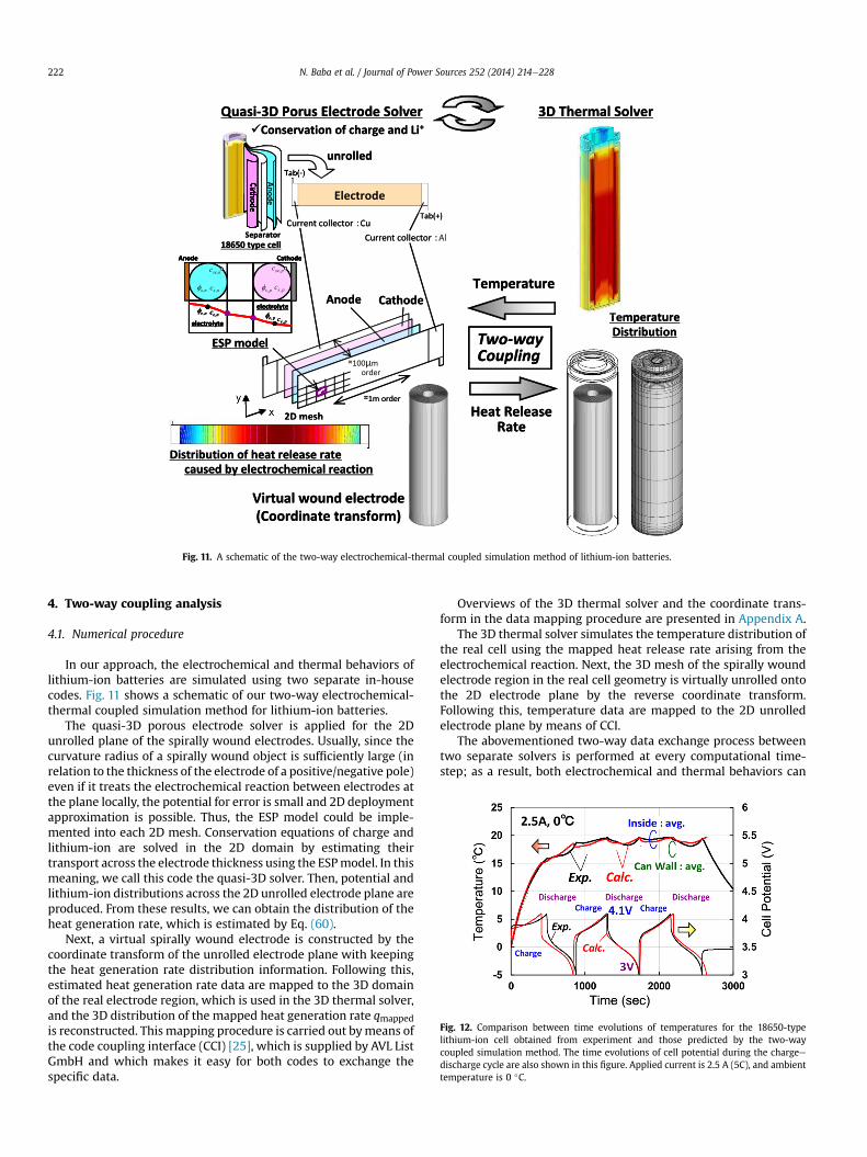
Fig. 11. A schematic of the two-way electrochemical-thermal coupled simulation method of lithium-ion batteries.

Fig. 12. Comparison between time evolutions of temperatures for the 18650-typelithium-ion cell obtained from experiment and those predicted by the two-waycoupled simulation method. The time evolutions of cell potential during the chargeedischarge cycle are also shown in this figure. Applied current is 2.5 A (5C), and ambienttemperature is 0 �C.

N. Baba et al. / Journal of Power Sources 252 (2014) 214e228222

4. Two-way coupling analysis

4.1. Numerical procedure

In our approach, the electrochemical and thermal behaviors oflithium-ion batteries are simulated using two separate in-housecodes. Fig. 11 shows a schematic of our two-way electrochemical-thermal coupled simulation method for lithium-ion batteries.

The quasi-3D porous electrode solver is applied for the 2Dunrolled plane of the spirally wound electrodes. Usually, since thecurvature radius of a spirally wound object is sufficiently large (inrelation to the thickness of the electrode of a positive/negative pole)even if it treats the electrochemical reaction between electrodes atthe plane locally, the potential for error is small and 2D deploymentapproximation is possible. Thus, the ESP model could be imple-mented into each 2D mesh. Conservation equations of charge andlithium-ion are solved in the 2D domain by estimating theirtransport across the electrode thickness using the ESPmodel. In thismeaning, we call this code the quasi-3D solver. Then, potential andlithium-ion distributions across the 2D unrolled electrode plane areproduced. From these results, we can obtain the distribution of theheat generation rate, which is estimated by Eq. (60).

Next, a virtual spirally wound electrode is constructed by thecoordinate transform of the unrolled electrode plane with keepingthe heat generation rate distribution information. Following this,estimated heat generation rate data are mapped to the 3D domainof the real electrode region, which is used in the 3D thermal solver,and the 3D distribution of the mapped heat generation rate qmappedis reconstructed. This mapping procedure is carried out bymeans ofthe code coupling interface (CCI) [25], which is supplied by AVL ListGmbH and which makes it easy for both codes to exchange thespecific data.

Overviews of the 3D thermal solver and the coordinate trans-form in the data mapping procedure are presented in Appendix A.

The 3D thermal solver simulates the temperature distribution ofthe real cell using the mapped heat release rate arising from theelectrochemical reaction. Next, the 3D mesh of the spirally woundelectrode region in the real cell geometry is virtually unrolled ontothe 2D electrode plane by the reverse coordinate transform.Following this, temperature data are mapped to the 2D unrolledelectrode plane by means of CCI.

The abovementioned two-way data exchange process betweentwo separate solvers is performed at every computational time-step; as a result, both electrochemical and thermal behaviors can

N. Baba et al. / Journal of Power Sources 252 (2014) 214e228 223

be reproduced simultaneously. Additionally, physical properties areupdated depending on the temperature at every computationaltime-step.

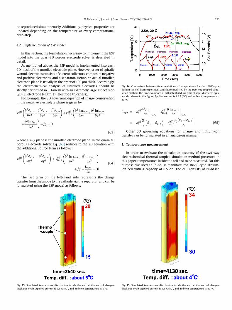
Fig. 14. Comparison between time evolutions of temperatures for the 18650-typelithium-ion cell from experiment and those predicted by the two-way coupled simu-lation method. The time evolutions of cell potential during the chargeedischarge cycleare also shown in this figure. Applied current is 2.5 A (5C), and ambient temperature is20 �C.

4.2. Implementation of ESP model

In this section, the formulation necessary to implement the ESPmodel into the quasi-3D porous electrode solver is described indetail.

As mentioned above, the ESP model is implemented into each2D mesh of the unrolled electrode plane. However, a set of spirallywound electrodes consists of current collectors, composite negativeand positive electrodes, and a separator. Hence, an actual unrolledelectrode plane is usually in the order of 100 mm thick. Accordingly,the electrochemical analysis of unrolled electrodes should bestrictly performed in 3D-mesh with an extremely large aspect ratioL/D (L: electrode length, D: electrode thickness).

For example, the 3D governing equation of charge conservationin the negative electrolyte phase is given by

keffn

v2fe;n

vx2þv2fe;n

vy2þv2fe;n

vz2

!þkeffD;n

v2 lnce;n

vx2þv2 lnce;n

vy2

þv2 lnce;nvz2

!þ jLin ¼ 0

(63)

where a xey plane is the unrolled electrode plane. In the quasi-3Dporous electrode solver, Eq. (63) reduces to the 2D equation withthe additional source term as follows:

keffn

v2fe; n

vx2þ v2fe; n

vy2

!þ keffD; n

v2 ln ce;n

vx2þ v2 ln ce; n

vy2

!

þ jLin � isepaLn

¼ 0

(64)

The last term on the left-hand side represents the chargetransfer from the anode to the cathode via the separator, and can beformulated using the ESP model as follows:

Fig. 13. Simulated temperature distribution inside the cell at the end of chargeedischarge cycle. Applied current is 2.5 A (5C), and ambient temperature is 0 �C.

isepa ¼ �keffnvfe; n

vz

����z¼Ln

� keffD; nv ln ce; n

vz

����z¼Ln

¼ �keffn3Ln

�f1 � fe; n

�� keffD; n

3Ln

�c1 � ce; n

�c1

(65)

Other 3D governing equations for charge and lithium-iontransfer can be formulated in an analogous manner.

5. Temperature measurement

In order to evaluate the calculation accuracy of the two-wayelectrochemical-thermal coupled simulation method presented inthis paper, temperatures inside the cell had to bemeasured. For thispurpose, we used an in-house manufactured 18650-type lithium-ion cell with a capacity of 0.5 Ah. The cell consists of Ni-based

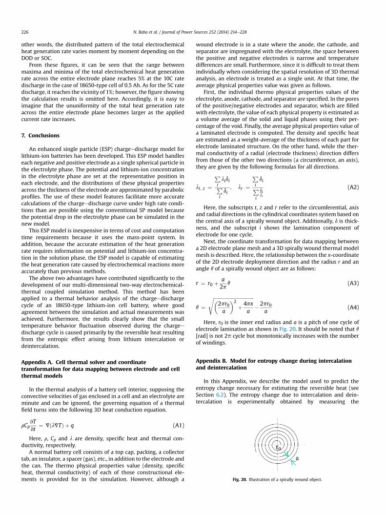
Fig. 15. Simulated temperature distribution inside the cell at the end of chargeedischarge cycle. Applied current is 2.5 A (5C), and ambient temperature is 20 �C.

Fig. 16. Comparison between time evolutions of temperatures for the 18650-typelithium-ion cell from experiment and those predicted by the two-way coupled simu-lation method. The time evolutions of cell potential during the chargeedischarge cycleare also shown in this figure. Applied current is 5 A (10C), and ambient temperature is20 �C.

N. Baba et al. / Journal of Power Sources 252 (2014) 214e228224

composite oxides positive and graphite negative. Experimentalconditions were set as follows. Ambient temperatures are 0 and20 �C. The chargeedischarge condition is Constant Current (CC)with no rest. Applied currents are 2.5 and 5.0 A. Cut-off voltages are4.1 V for charge and 3.0 V for discharge.

Two 18650-type lithium-ion cells were supplied for measure-ment purposes, while type-T (copper-constantan) thermocoupleswere used for the measurements themselves. The thermocoupleswere 0.13mm in diameter. Three thermocouples were inserted intoone cell in the axial direction, and another three were inserted intothe second cell along the radial direction. In addition, six thermo-couples were placed on the can wall of each cell.

6. Results and discussion

6.1. Comparisons between simulated results and measured results

Fig. 12 shows comparisons between the time evolutions oftemperatures of the 18650-type lithium-ion cell obtained viaexperiment and those calculated by the two-way coupled

Fig. 17. Simulated temperature distribution inside the cell at the end of chargeedischarge cycle. Applied current is 5 A (10C), and ambient temperature is 20 �C.

simulation method. The lower two sawtooth lines compare timevariations of cell potential. Applied current is 2.5 A (5C). Theambient temperature and the initial temperature of the preparedcell were set at 0 �C. It should be noted that the temperatures in thisfigure reflect the average value of the measured temperaturesbecause differences at each measured point were within one de-gree, as shown in Fig. 13. However, the maximum temperaturedifference across the entire cell was about five degrees because ofthe large heat mass at the upper side. It is noteworthy that the timevariations of temperature measurements, both inside the cell andon the can wall, were simulated within three degrees of accuracy,and that the simulation of the temperature fluctuation during thechargeedischarge cycle could be performed with high accuracy.

Other validation calculation results are exhibited in thefollowing figures. Fig. 14 shows the results in a case where theapplied current is 2.5 A (5C) and ambient temperature is 20 �C.From Fig. 15, it can be seen that the maximum temperature dif-ference across the entire cell becomes about four degrees at the endof the chargeedischarge cycle in this case. Additionally, Fig. 16shows the result of a case where the applied current is 5 A (10C)and ambient temperature is 20 �C, in which case the maximumtemperature difference across the entire cell reaches about ninedegrees, as shown in Fig. 17.

Based on these validation results, it can be seen that the two-way electrochemical-thermal coupled simulation method pre-sented in this paper is capable of simulating temperatures insidethe cell and on the can wall with an accuracy level within a fewdegrees.

6.2. Contribution of each heat release source term

In this section, we will devote a little more space to discussingthe contribution of each heat source term to total electrochemicalheat release rate.

As previously mentioned, the local electrochemical heat releaserate consists of three heat source terms that are expressed in Eq. (1)and/or Eq. (60):

Qelchem ¼ Qohmic þ Qirrev þ Qrev (66)

The first term on the right-hand side refers to the ohmic heatcaused by ionic resistance. The second term represents the irre-versible heat arising from overpotential and film resistance. Thethird term expresses the reversible heat resulting from the entropiceffect of lithium intercalation or deintercalation. These three termsare formulated as follows:

Qohmic ¼X

j¼n; p

�seffj Vfs; j$Vfs; j

�þ

Xj¼n; sep; p

�keffj Vfe; j$Vfe; j

þ keffD; jV ln ce; j$Vfe; j

�(67)

Qirrev ¼X

j¼n; p

as; jin; j�fs; j � fe; j � Uj

�(68)

Qrev ¼X

j¼n; p

as; jin; jTvUj

vT(69)

Fig. 18 displays the effect of each three heat source term on timevariations of temperature of the cell during the chargeedischargecycle at the 5C rate (2.5 A), 0 �C. Here, only one-cycle dischargeecharge process is shown. As indicated in Fig. 18(a), a small tem-perature fluctuation is observed inside the cell. Fig. 18(b) and (c)

Fig. 18. Effect of each heat source term on time variations of temperature of the cell during the chargeedischarge cycle at the 5C rate (2.5 A), 0 �C. The small fluctuation of thetemperature behavior is mainly caused by the reversible heat resulting from entropic effect due to lithium-ion intercalation or deintercalation.

Fig. 19. Time evolutions of distributed patterns of the total electrochemical heat release rate across the entire electrode plane during discharge process at the 10C rate (5 A), 20 �C.

N. Baba et al. / Journal of Power Sources 252 (2014) 214e228 225

shows the time variations of the contribution ratio for each of thethree heat source terms in relation to the total electrochemical heatrelease rate during the discharge and charge process, respectively.From these figures, it is clear that the ohmic heat is similar in valuebetween discharge and charge and remains constant over theentire process. In addition, it can be seen that the irreversible heatis also similar in value between both processes and maintainsnearly constant. As a result, a remarkable difference is observed inthe reversible heat, which is expressed by Eq. (69).

The time variation of the total electrochemical heat release rateis directly reflected in the thermal behavior of the cell, as shown inFig. 18. Furthermore, the reversible heat governs the time variationbehavior of the heat generation rate. Accordingly, these results leadto the conclusion that the small fluctuation noted in the tempera-ture behavior is caused primarily by the reversible heat.

Reversible heat variations depend on the local state of charge(SOC) of the anode and cathode active materials during thedischarge and charge process. In order to evaluate the reversibleheat, the entropy change DS value of the active materials, which isrelated to the derivative of the open circuit potential (OCP) withrespect to temperature, is necessary. In this study, instead ofmeasuring DS directly, we used a model formulation that predicts

the entropy change based on experimental data of the OCP. Detailsof the model used for entropy change are provided in Appendix B.

6.3. Distribution of heat generation rate

In the two-way coupled simulation method presented in thispaper, the electrochemical phenomena of lithium-ion batteries aresimulated using the quasi-3D porous electrode solver. Hence, the2D distributed information of a heat generation rate arising fromelectrochemical reactions across an entire electrode plane can beobtained.

Fig. 19 shows the distribution of a heat generation rate across anentire unrolled electrode plane. Fig. 19(a) shows comparisons be-tween charge and discharge curves obtained from experiments andsimulated results at the 10C rate (5 A), 20 �C, while Fig. 19(b) and (c)shows distributed patterns of the total electrochemical heat gen-eration rate when the DOD in the discharge process equals 30% and50%, respectively.

At DOD ¼ 30%, the maximum heat generation rate puts in anappearance at the end near the negative tab, while the minimumvalue occurs at the central region. In contrast, the distributedpattern of the heat generation rate turns around at DOD ¼ 50%. In

N. Baba et al. / Journal of Power Sources 252 (2014) 214e228226

other words, the distributed pattern of the total electrochemicalheat generation rate varies moment by moment depending on theDOD or SOC.

From these figures, it can be seen that the range betweenmaxima and minima of the total electrochemical heat generationrate across the entire electrode plane reaches 5% at the 10C ratedischarge in the case of 18650-type cell of 0.5 Ah. As for the 5C ratedischarge, it reaches the vicinity of 1%; however, the figure showingthe calculation results is omitted here. Accordingly, it is easy toimagine that the ununiformity of the total heat generation rateacross the entire electrode plane becomes larger as the appliedcurrent rate increases.

7. Conclusions

An enhanced single particle (ESP) chargeedischarge model forlithium-ion batteries has been developed. This ESP model handleseach negative and positive electrode as a single spherical particle inthe electrolyte phase. The potential and lithium-ion concentrationin the electrolyte phase are set at the representative position ineach electrode, and the distributions of these physical propertiesacross the thickness of the electrode are approximated by parabolicprofiles. The use of these model features facilitate more accuratecalculations of the chargeedischarge curve under high rate condi-tions than are possible using the conventional SP model becausethe potential drop in the electrolyte phase can be simulated in thenew model.

This ESP model is inexpensive in terms of cost and computationtime requirements because it uses the mass-point system. Inaddition, because the accurate estimation of the heat generationrate requires information on potential and lithium-ion concentra-tion in the solution phase, the ESP model is capable of estimatingthe heat generation rate caused by electrochemical reactions moreaccurately than previous methods.

The above two advantages have contributed significantly to thedevelopment of our multi-dimensional two-way electrochemical-thermal coupled simulation method. This method has beenapplied to a thermal behavior analysis of the chargeedischargecycle of an 18650-type lithium-ion cell battery, where goodagreement between the simulation and actual measurements wasachieved. Furthermore, the results clearly show that the smalltemperature behavior fluctuation observed during the chargeedischarge cycle is caused primarily by the reversible heat resultingfrom the entropic effect arising from lithium intercalation ordeintercalation.

Fig. 20. Illustration of a spirally wound object.

Appendix A. Cell thermal solver and coordinatetransformation for data mapping between electrode and cellthermal models

In the thermal analysis of a battery cell interior, supposing theconvective velocities of gas enclosed in a cell and an electrolyte areminute and can be ignored, the governing equation of a thermalfield turns into the following 3D heat conduction equation.

rCpvTvt

¼ VðlVTÞ þ q (A1)

Here, r, Cp and l are density, specific heat and thermal con-ductivity, respectively.

A normal battery cell consists of a top cap, packing, a collectortab, an insulator, a spacer (gas), etc., in addition to the electrode andthe can. The thermo physical properties value (density, specificheat, thermal conductivity) of each of those constructional ele-ments is provided for in the simulation. However, although a

wound electrode is in a state where the anode, the cathode, andseparator are impregnated with the electrolyte, the space betweenthe positive and negative electrodes is narrow and temperaturedifferences are small. Furthermore, since it is difficult to treat themindividually when considering the spatial resolution of 3D thermalanalysis, an electrode is treated as a single unit. At that time, theaverage physical properties value was given as follows.

First, the individual thermo physical properties values of theelectrolyte, anode, cathode, and separator are specified. In the poresof the positive/negative electrodes and separator, which are filledwith electrolyte, the value of each physical property is estimated asa volume average of the solid and liquid phases using their per-centage of the void. Finally, the average physical properties value ofa laminated electrode is computed. The density and specific heatare estimated as a weight-average of the thickness of each part forelectrode laminated structure. On the other hand, while the ther-mal conductivity of a radial (electrode thickness) direction differsfrom those of the other two directions (a circumference, an axis),they are given by the following formulas for all directions.

lt; z ¼

PilidiP

idi

; lr ¼

PidiP

i

dili

(A2)

Here, the subscripts t, z and r refer to the circumferential, axisand radial directions in the cylindrical coordinates system based onthe central axis of a spirally wound object. Additionally, d is thick-ness, and the subscript i shows the lamination component ofelectrode for one cycle.

Next, the coordinate transformation for data mapping betweena 2D electrode plane mesh and a 3D spirally wound thermal modelmesh is described. Here, the relationship between the x-coordinateof the 2D electrode deployment direction and the radius r and anangle q of a spirally wound object are as follows:

r ¼ r0 þa2p

q (A3)

q ¼ffiffiffiffiffiffiffiffiffiffiffiffiffiffiffiffiffiffiffiffiffiffiffiffiffiffiffiffiffiffiffiffiffiffi�2pr0a

�2þ 4px

a

s� 2pr0

a(A4)

Here, r0 is the inner end radius and a is a pitch of one cycle ofelectrode lamination as shown in Fig. 20. It should be noted that q[rad] is not 2p cycle but monotonically increases with the numberof windings.

Appendix B. Model for entropy change during intercalationand deintercalation

In this Appendix, we describe the model used to predict theentropy change necessary for estimating the reversible heat (seeSection 6.2). The entropy change due to intercalation and dein-tercalation is experimentally obtained by measuring the

Fig. 21. Comparison of the model prediction and experimental results. (a) Open circuit potential U. (b) Entropy change (vU/vT) ¼ DS/F. The solid line indicates the present results, thedashed line indicates the model prediction by Wong and Newman [29], and the symbol indicates the experimental results provided by Thomas et al. [28].

N. Baba et al. / Journal of Power Sources 252 (2014) 214e228 227

temperature dependence of the open circuit potential (OCP).However, performing this measurement is difficult because it takesa significant amount of time to reach the equilibrium state (atwhich the OCP can be measured) after the temperature is changed.In contrast, the model described in this Appendix predicts thetemperature dependence based solely on the OCP data at a fixedtemperature.

The model is premised on the assumption that the active ma-terial consists of N independent components that have differentreaction properties. This is a model for describing the stepwisechange of the OCP depending on the SOC, which is used by Zhanget al. [26] to derive a kinetic model.

We begin by introducing several variables into the modeldescription. Let q be the ratio of the number of intercalated lithiumatoms to the total number of the sites in the active material. Inaddition, let Qk and qk denote the ratios of the number of the sites,and the number of lithium atoms in kth component, respectively, tothe total number of sites in the active material:

XNk¼1

Qk ¼ 1;XNk¼1

qk ¼ 0: (B1)

Following the discussion in Ref. [26], starting from the ButlereVolmer kinetics for multi-component material, the following rela-tion, which holds at the equilibrium state, is derived:

U ¼ U0k þ RT

Fln�Qk � qk

qk

�xk

; (B2)

where U0k is a quantity related to the reaction rate, and xk is the

order of the reaction of the kth component. Solving Eq. (B2) withrespect to qk and substituting into Eq. (B1) yields

q ¼XNk¼1

Qk

1þ exp�

FxjRT

�U � U0

k

�� : (B3)

This relationship between q and U with the model parametersQk, U0

k , and xk coincides with the OCP model proposed semi-empirically by Verbrugge and Koch in their work on modelinggraphite electrodes [27]. Differentiation of Eq. (B3) with respect to Tgives the quantity related to the entropy change DS through (vU/vT) ¼ DS/F:

T�vUvT

�¼PN

k¼1QkEk

xkð1þEjÞ2�U � U0

k

�PN

k¼1QkEk

xkð1þEjÞ2; (B4)

where

Ek ¼ exp�

FxkRT

�U � U0

k

��: (B5)

Once we have the (B3) relationship fitted to a qeU curvemeasured experimentally, the predicted values of entropy changeare drawn immediately using the same set of model parametersQk,U0k , and xk. Note that the coefficient U0

k , which is related to the re-action rate, is intrinsically a function of temperature. In the abovederivation, however, we ignore the dependency of U0

k on temper-ature in view of the fact that the dependency vanishes in caseswhere the frequency factor value is common to the anodic andcathodic reaction.

The adequacy of the model is assessed by comparison with theexperimental results by Thomas et al. [28] They measured the OCPand vU/vT of lithium manganese spinel (LiyMn2O4) at variousvalues of q. The values of the model parameters Qk, U0

k , and xk weredetermined by fitting Eq. (B3) with N ¼ 6 to the experimental dataof the OCP. The method we employed to accomplish this is thestandard nonlinear general reduced gradient (GRG) optimizationalgorithm. We then estimated the values of vU/vT using Eq. (B4).Fig. 21 compares the results of the present model and Ref. 27.Although the present model underestimates the value of (vU/vT) ¼ DS/F in the intermediate region of q, the overall entropychange trend is captured well. In the figure, the results of themodel provided by Wong and Newman [29] are also shown. Intheir model, both the OCP and vU/vT are predicted. The accuracy ofthe entropy change is almost the same as the present model,whereas the reproduction of the OCP of the present model is moreaccurate.

List of symbols

as specific interfacial area of an electrode (m2 m�3)ce Liþ concentration in the electrolyte phase (mol m�3)cs Li concentration in the solid particles (mol m�3)cse Li concentration at the surface of the solid particles

(mol m�3)

N. Baba et al. / Journal of Power Sources 252 (2014) 214e228228

De diffusion coefficient of Liþ in the electrolyte phase(m2 s�1)

Ds diffusion coefficient of Liþ in the solid phase (m2 s�1)F Faraday’s constant (96,487C mol�1)Iapp applied current density (A m�2)i0 exchange current density (A m�2)in superficial current density (A m�2)j local volumetric transfer current density due to charge

transfer (A m�3)lse diffusion length of Liþ from solideelectrolyte interface

into solid phase (m)L thickness of n, sep or p (m)q heat generation rate (W m�3)R universal gas constant (8.3143 J/(mol�1$K))Rf film resistance on an electrode surface (U m2)r radial coordinate (m)rs radius of the spherical particles (m)T absolute temperature (K)t time (s)t�þ transference number of Liþ in solutionU open-circuit potential of an electrode reaction (V)x, y coordinates on the unrolled electrode plane (m)z coordinate across the thickness of the electrode (m)

Greek symbolsaa,ac anodic and cathodic transfer coefficients for an electrode

reactionε volume fraction of a phaseh surface overpotential of an electrode reaction (V)k conductivity of the electrolyte (S m�1)kD diffusional conductivity of the electrolyte (A m�1)s conductivity of the electrode (S m�1)ɸs electrical potential in the solid phase (V)ɸe electrical potential in the electrolyte phase (V)

Subscript and superscripteff effective

j n or pLi lithium speciesn negative electrodep positive electrodesep separator

References

[1] W.B. Gu, C.Y. Wang, Lithium Batteries, PV 99-25, in: The Electrochemical So-ciety Proceedings, 1999, pp. 748e762.

[2] W.B. Gu, C.Y. Wang, J. Electrochem. Soc. 147 (2000) 2910e2922.[3] L. Rao, J. Newman, J. Electrochem. Soc. 144 (1997) 2697e2704.[4] P.M. Gomadam, J.W. Weidner, R.A. Dougal, R.E. White, J. Power Sources 110

(2002) 267e284.[5] C.R. Pals, J. Newman, J. Electrochem. Soc. 142 (1995) 3274e3281.[6] C.R. Pals, J. Newman, J. Electrochem. Soc. 142 (1995) 3282e3288.[7] Y. Chen, J.W. Evans, J. Electrochem. Soc. 140 (1993) 1833e1838.[8] Y. Chen, J.W. Evans, J. Electrochem. Soc. 141 (1994) 2947e2955.[9] Y. Chen, J.W. Evans, J. Electrochem. Soc. 143 (1996) 2708e2712.

[10] U.S. Kim, C.B. Shin, C.S. Kim, J. Power Sources 180 (2008) 909e916.[11] U.S. Kim, C.B. Shin, C.S. Kim, J. Power Sources 189 (2009) 841e846.[12] R. Spotnitz, J. Franklin, J. Power Sources 113 (2003) 81e100.[13] G.H. Kim, A. Pesaran, R. Spotnitz, J. Power Sources 170 (2007) 476e489.[14] M. Doyle, T.F. Fuller, J. Newman, J. Electrochem. Soc. 140 (1993) 1526e

1533.[15] D. Bernardi, E. Pawlikowski, J. Newman, J. Electrochem. Soc. 132 (1985)

5e12.[16] B.S. Haran, B.N. Popov, R.E. White, J. Power Sources 75 (1998) 56e63.[17] V.R. Subramanian, J.A. Ritter, R.E. White, J. Electrochem. Soc. 148 (2001)

E444eE449.[18] G. Ning, B.N. Popov, J. Electrochem. Soc. 151 (2004) A1584eA1591.[19] S. Santhanagopalan, Q. Guo, P. Ramadass, R.E. White, J. Power Sources 156

(2006) 620e628.[20] Q. Zhang, R.E. White, J. Power Sources 165 (2007) 880e886.[21] Q. Zhang, R.E. White, J. Power Sources 179 (2008) 793e798.[22] C.Y. Wang, W.B. Gu, B.Y. Liaw, J. Electrochem. Soc. 145 (1998) 3407e3417.[23] M. Doyle, J. Newman, A.S. Gozdz, C.N. Schmutz, J.-M. Tarascon, J. Electrochem.

Soc. 143 (1996) 1890e1903.[24] C.Y. Wang, V. Srinivasan, J. Power Sources 110 (2002) 364e376.[25] AVL FIRE� Version, 2009. Manual.[26] Q. Zhang, Q. Guo, R.E. White, J. Electrochem. Soc. 153 (2006) A301eA309.[27] M.W. Verbrugge, B.J. Koch, J. Electrochem. Soc. 150 (2003) A374eA384.[28] K.E. Thomas, C. Bogatu, J. Newman, J. Electrochem. Soc. 148 (2001) A570e

A575.[29] W.C. Wong, J. Newman, J. Electrochem. Soc. 149 (2002) A493eA498.