1

Routing & Switching for Internet

2

Outline Introduction – IP Protocol Classful IP Addresses and CIDR IP Routing Protocols and Algorithms Hardware Routing Schemes Multiple Protocol Label Switching

3

Introduction - IP Protocol

4

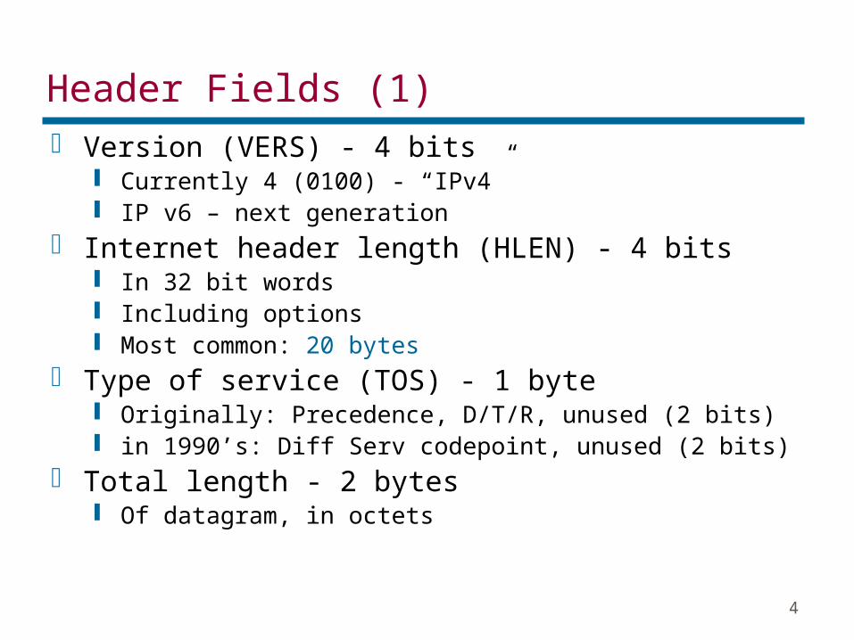
Header Fields (1) Version (VERS) - 4 bits

Currently 4 (0100) - “IPv4” IP v6 – next generation

Internet header length (HLEN) - 4 bits In 32 bit words Including options Most common: 20 bytes

Type of service (TOS) - 1 byte Originally: Precedence, D/T/R, unused (2 bits) in 1990’s: Diff Serv codepoint, unused (2 bits)

Total length - 2 bytes Of datagram, in octets

5

Header Fields (2) Identification

Sequence number Used with addresses and user protocol to identify

datagram uniquely

Flags More bit Don’t fragment

Fragmentation offset Time to live Protocol

Next higher layer to receive data field at destination

6

Header Fields (3) Header checksum

Re-verified and recomputed at each router 16 bit ones complement sum of all 16 bit words in

header Set to zero during calculation

Source address Destination address Options Padding

To fill to multiple of 32 bits long

7

Options Security Source routing Route recording Stream identification Timestamping

8

Data Field Carries user data from next layer up Integer multiple of 8 bits long (octet) Max length of datagram (header plus data)

65,535 octets

9

Classful IP Addresses IP address

IPv4: 32-bit address dotted-quad or dotted decimal ex. 130.221.203.154 decimal = 82.DD.CB.9A hex = 1000 0010 . 1101 1101 . 1100 1011 . 1001 1010 binary only 232 (4,294,967,296) IPv4 addresses available

2 parts: netid & hostid

“Classful” addressing Class A Class B Class C Class D - Mulitcast Class E - Reserved for future use

10

Classful IP Addresses - Class A

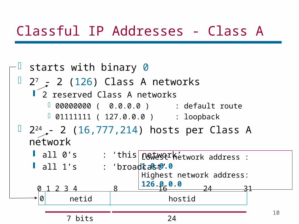
starts with binary 0 27 - 2 (126) Class A networks

2 reserved Class A networks00000000 ( 0.0.0.0 ) : default route01111111 ( 127.0.0.0 ) : loopback

224 - 2 (16,777,214) hosts per Class A network all 0’s : ‘this network’ all 1’s : ‘broadcast’

00 1 2 3 4 8 16 24 31

netid hostid

7 bits 24 bits

Lowest network address : 1.0.0.0Highest network address: 126.0.0.0

11

Classful IP Addresses - Class B

Start with 10 Second Octet also included in network address 214 = 16,384 class B addresses

1 00 1 2 3 4 8 15 16 24 31

netid hostid

14 bits 16 bits

Lowest address : 128.0.0.0Highest address: 191.255.0.0

12

Classful IP Addresses - Class C Start with 110 Second and third octet also part of network

address 221 = 2,097,152 addresses

1 1 00 1 2 3 7 15 23 24 31

netid hostid

21 bits 8 bits

Lowest address : 192.0.0.0Highest address: 223.255.255.0

13

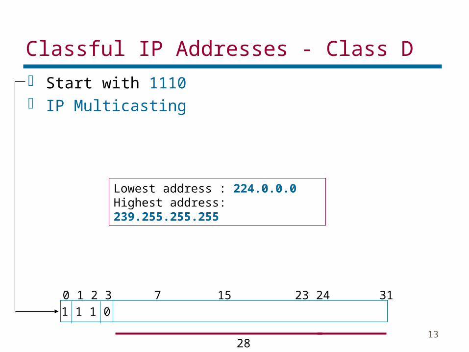
Classful IP Addresses - Class D Start with 1110 IP Multicasting

1 1 1 00 1 2 3 7 15 23 24 31

28 bits

Lowest address : 224.0.0.0Highest address: 239.255.255.255

14

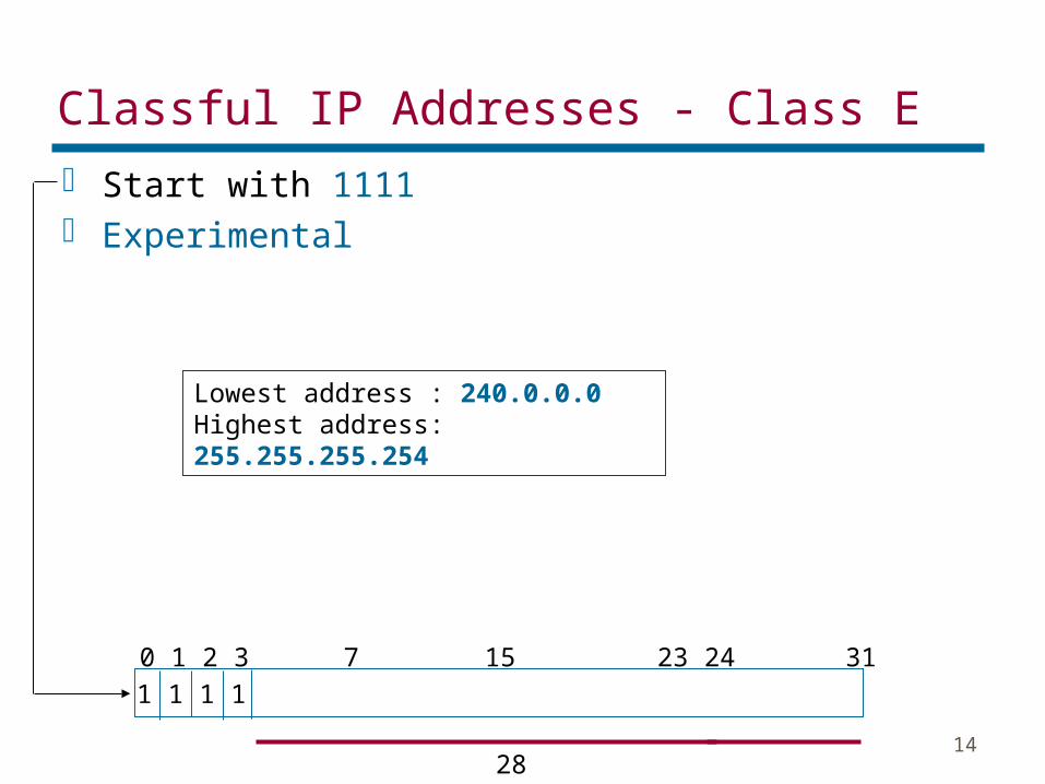
Classful IP Addresses - Class E Start with 1111 Experimental

1 1 1 10 1 2 3 7 15 23 24 31

28 bits

Lowest address : 240.0.0.0Highest address: 255.255.255.254

15

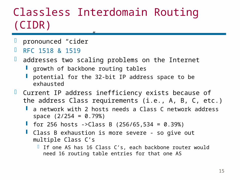
Classless Interdomain Routing (CIDR) pronounced “cider” RFC 1518 & 1519 addresses two scaling problems on the Internet

growth of backbone routing tables potential for the 32-bit IP address space to be exhausted

Current IP address inefficiency exists because of the address Class requirements (i.e., A, B, C, etc.) a network with 2 hosts needs a Class C network address space

(2/254 = 0.79%) for 256 hosts ->Class B (256/65,534 = 0.39%) Class B exhaustion is more severe - so give out multiple Class

C’s If one AS has 16 Class C’s, each backbone router would need 16

routing table entries for that one AS

16

CIDR CIDR helps to aggregate routes

hand out contiguous blocks of Class C addresses ex: 192.4.16 - 192.4.31

16 Class C’s They all start with 1100 0000 - 0000 0100 - 0001 . . . looks like a 20-bit network number - something between a

Class B and a Class C each block must contain a number of Class C networks that

is a power of 2

need a routing protocol that can deal with these “classless” addresses (i.e., a non-standard network number) BGP version 4 is able to do this Network numbers are represented by (length, value) pairs

example above would have length = 20 similar to the (mask, value) for subnets

17

IP Routing In a packet-switched network, routing relates to

the process of choosing a link to send the packets over. Router: the computer that makes this choice.

an internet is composed of multiple physical networks interconnected by computers (or network devices) called routers

forwarding: take a packet, look at its destination address, consult a table, send packet to its destination based on that table

routing: process which builds the forwarding tables

18

IP Routing For routing to scale, a hierarchical routing

infrastructure is used (Internet) Autonomous System (AS)

a group of routers exchanging info with a common routing protocol

a set of routers and networks managed by a single organization

connected (except during failures): a path exists between any two pair of nodes

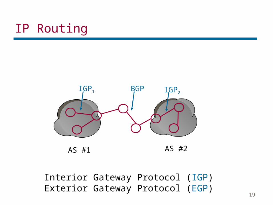
Interior Gateway Protocols (IGPs) - within an AS Exterior Gateway Protocols (EGPs) - between ASs

19

IP Routing

AS #1 AS #2

IGP1 IGP2BGP

Interior Gateway Protocol (IGP)Exterior Gateway Protocol (EGP)

20

IP Routing routing: graph theory problem

nodes : hosts, switches, routers, or networks initial case: consider all nodes as routers

edges of graph: network links (assume undirected)

cost is associated with each edge relates to desirability of sending traffic over particular link routing problem: find the lowest-cost path between any

two nodes cost = sum of costs of all of the edges that form the path

CB

A

DE F4

9

3 6

1 21

node (router)

edge (link)

cost

21

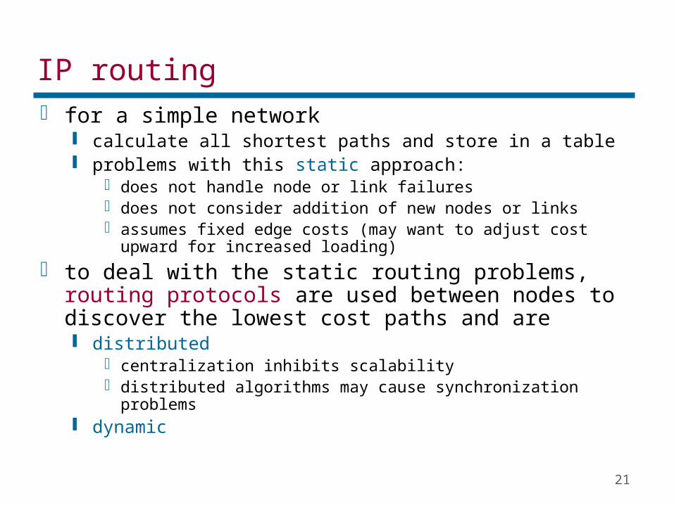
IP routing for a simple network

calculate all shortest paths and store in a table problems with this static approach:

does not handle node or link failures does not consider addition of new nodes or links assumes fixed edge costs (may want to adjust cost upward

for increased loading)

to deal with the static routing problems, routing protocols are used between nodes to discover the lowest cost paths and are distributed

centralization inhibits scalability distributed algorithms may cause synchronization

problems dynamic

22

IP intradomain routing Look at two main classes of IGPs

distance vector (RIP) link state (OSPF)

assume all edge costs are known

23

Routing Information Protocol (RIP) built on a Distance-Vector algorithm

also called Bellman-Ford algorithm, after the inventors each node constructs a one-dimensional array (a vector)

of the “distances” (costs) to all of the other nodes and distributes the vector to its immediate neighbors

assumes that each node knows the cost of the links to its immediate (directly connected) neighbors

a link outage is assigned an infinite cost assume each link cost = 1, so now least-cost path is the

fewest number of router hops One of the most widely-used routing protocols RFC 1058

24

RIP example

Info Stored Distance to reach node at node A B C D E F G

A 0 1 1 1 1 B 1 0 1 C 1 1 0 1 D 1 0 1 E 1 0 F 1 0 1 G 1 1 0

initial distances/costs stored at each node

Destination Cost NextHop

B 1 BC 1 CD -E 1 EF 1 FG -

initial routing table at node A

25

RIP example, cont.

Info Stored Distance to reach node at node A B C D E F G

A 0 1 1 2 1 1 2B 1 0 1 2 2 2 3C 1 1 0 1 2 2 2D 2 2 1 0 3 2 1 E 1 2 2 3 0 2 3 F 1 2 2 2 2 0 1 G 2 3 2 1 3 1 0

final distances/costs stored at each node

Destination Cost NextHop

B 1 BC 1 CD 2 CE 1 EF 1 FG 2 F

final routing table at node A

26

RIP example, cont in the absence of any topology changes, only a few

exchanges are required between neighbors before each node has completed its routing table

convergence: the process of getting consistent routing information to all of the nodes

there is no one node in the network that has all of the information in the complete routing table

each node only has knowledge of its own routing table each node has a consistent view of the network in the

absence of any centralized authority routing updates

periodic (seconds to minutes) triggered

27

RIP, example RIP packets advertise costs to reach networks

(rather than routers/ nodes)

RIP packet format

command: ‘1’ (request), ‘2’ (reply)version: ‘1’ (or ‘2’ for RIPv2)address family: ‘2’ (IP)address: IP addressdistance: cost metric - hop count

up to 25 routes per RIP messagewell-known RIP port: UDP 520

28

RIP RIP messages carried in UDP datagrams RIP version 2 (RFC 1388)

RIP-2 pass additional information

routing domain, route tag, subnet mask interoperable with RIP

cisco’s proprietary distance-vector Interior Gateway Routing Protocol (IGRP)

29

Open Shortest Path First (OSPF) another intradomain or interior gateway protocol (IGP) Link-state ‘Open’ : non-proprietary (IETF) vs. proprietary EIGRP (cisco)

RFC 1247 each node is assumed to be capable of finding the state of

the link to its neighbors (up or down) and the cost of each link

assume reliable dissemination of link-state info

reliable flooding (all of node’s L-S info to all attached nodes) update packet (link-state packet [LSP])

calculation of routes from the sum of all the accumulated link-state knowledge

Dijkstra’s shortest-path algorithm

30

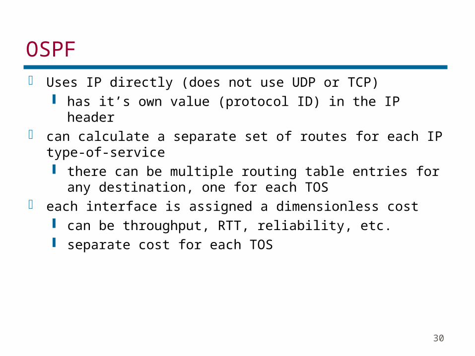
OSPF Uses IP directly (does not use UDP or TCP)

has it’s own value (protocol ID) in the IP header can calculate a separate set of routes for each IP type-of-

service there can be multiple routing table entries for any

destination, one for each TOS each interface is assigned a dimensionless cost

can be throughput, RTT, reliability, etc. separate cost for each TOS

31

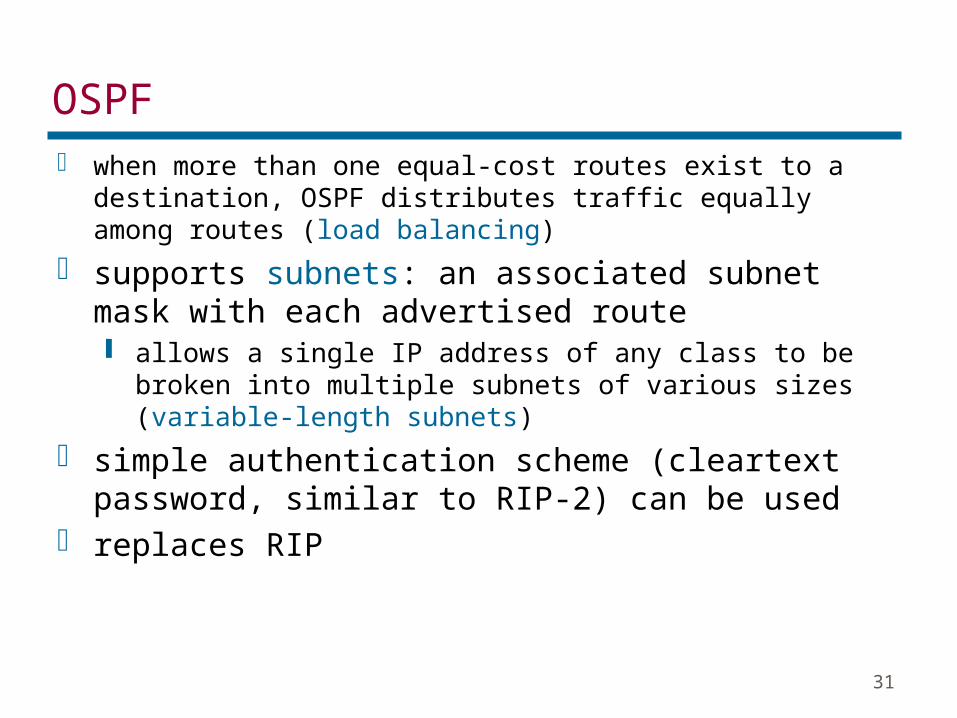
OSPF when more than one equal-cost routes exist to a

destination, OSPF distributes traffic equally among routes (load balancing)

supports subnets: an associated subnet mask with each advertised route allows a single IP address of any class to be broken into

multiple subnets of various sizes (variable-length subnets)

simple authentication scheme (cleartext password, similar to RIP-2) can be used

replaces RIP

32

Exterior Gateway Protocols (EGPs) interdomain routing protocols used between routers of different AS’s historically, the predominant EGP was a protocol

called EGP (confusing) the newer EGP is the Border Gateway Protocol

(BGP) version 3 (RFC 1267) RFC 1268 (use of BGP in the Internet) version 4 (RFC 1654)

message types (RFC 1771) updates sent using TCP

33

Bellman-Ford Algorithm(1/3)

1

2

3

4

5

1

4

1 2

8

2

4 2

1Source Node

Shortest paths problemarcs lengths as indicated

)(hiD

Definition

is the shortest (≤h) path length from node 1 to node i

Bellman-Ford Algorithm

Initially,1,)0( iallforDi

For each successive h≥0,

1],[min )()1( iallfordDD jihj

j

hi

Example I

34

Bellman-Ford Algorithm(2/3)

1

2

3

4

5

0)2(1 D

1)2(2 D 9)2(

4 D

6)2(5 D2)2(

3 D

Shortest paths usingat most 2 arcs

1

2

3

4

5

0)1(1 D

1)1(2 D )1(

4D

)1(5D4)1(

3 D

Shortest paths usingat most 1 arcs

35

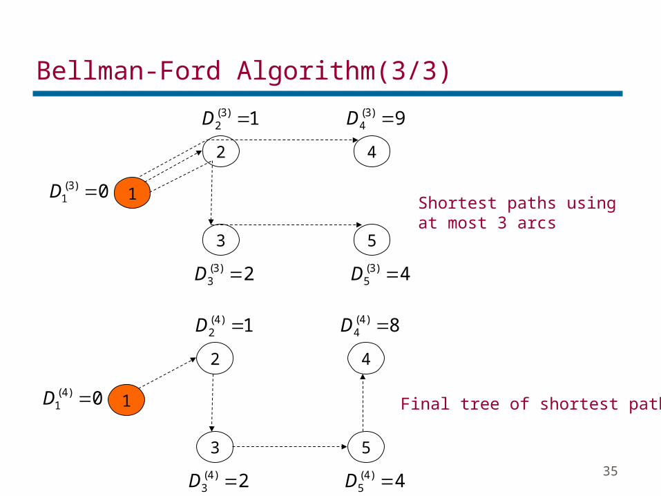
Bellman-Ford Algorithm(3/3)

Final tree of shortest paths1

2

3

4

5

0)4(1 D

1)4(2 D 8)4(

4 D

4)4(5 D2)4(

3 D

1

2

3

4

5

0)3(1 D

1)3(2 D 9)3(

4 D

4)3(5 D2)3(

3 D

Shortest paths usingat most 3 arcs

36

Dijkstra’s Algorithm(1/3)

Initially P={1}, D1=0, and 1for 1 jdD jj

Step1. (Find the closest node). Find such thatPij

Pji DD

min

Set . If P contains all nodes then stop ;the algorithm is complete

}{: iPP

ijijj dDDD ,min:

Step2. (Updating of labels). For all setPj

Go to Step1.

37

Dijkstra’s Algorithm(2/3) Example of Dijkstra’s

Algorithm

1

2

4

3

5

1

4

1

3

1

1

2

6

4

),( jiallfordd jiij

38

Dijkstra’s Algorithm(3/3)

1

2

4

12 D

44 D

3

5

43 D

25 DP = {1,2}

1

2

4

3

5

12 D 33 D

34 D 25 D

6

66 D

P = {1,2,5}

1

2

4

3

5

6

12 D

34 D 25 D

56 D

33 D

P = {1,2,3,4,5}

39

IP Address Lookup Algorithms –

Hardware Routing Schemes

40

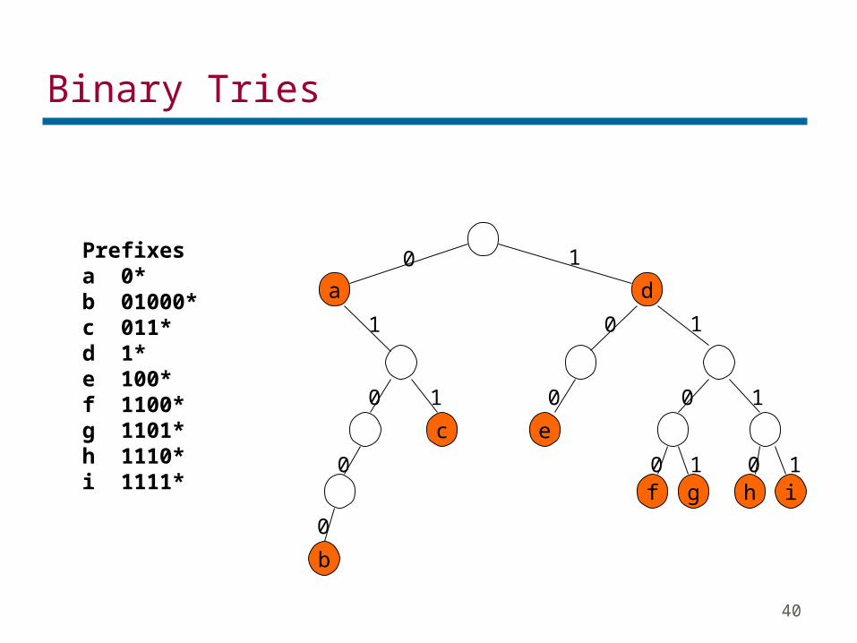
Binary Tries

Prefixesa 0*b 01000*c 011*d 1*e 100*f 1100*g 1101*h 1110*i 1111*

a d

c

b

e

h if g

0

0

0

0

0

0

0

0 0

1

1

1 1

1

11

41

Path-Compressed Trie

Prefixesa 0*b 01000*c 011*d 1*e 100*f 1100*g 1101*h 1110*i 1111*

a d

ec

h if g

0

0

0

0 0

1

1 1

1

11

b

0

1

3 2

3

4 4

Legend: x indicates to inspect which bit

42

Disjoint-prefix Binary Trie

Prefixesa 0*b 01000*c 011*d 1*e 100*f 1100*g 1101*h 1110*i 1111*

c

b

e

h if g

0

0

0

0

0

0

0

0 0

1

1

1 1

1

11

a1

0

a3

1

a2

1

d1

1

Leaf pushing Disjoint prefixes do not overlap No prefix is itself a prefix of another

43

Variable-stride Multibit Trie

a

c

01 10

a d d

00 11

c

b

ihgfe

00

0 1

0 101 1011 00 11

01 10

stride=2stride=1

Prefixesa 0*b 01000*c 011*d 1*e 100*f 1100*g 1101*h 1110*i 1111*

Reduced number of memory accesses Greater wasted space

44

Caching Addresses

CPU

MAC

LocalBuffer

Memory

LineCard

DMA

MAC

LocalBuffer

Memory

Fast Path

Slow Path

Advantages Increased average lookup performance

Disadvantages Decreased locality in backbone traffic Cache size Cache management overhead Hardware implementation difficult

LineCard

LocalBuffer

Memory

LineCard

DMA DMA

MAC

BufferMemory

45

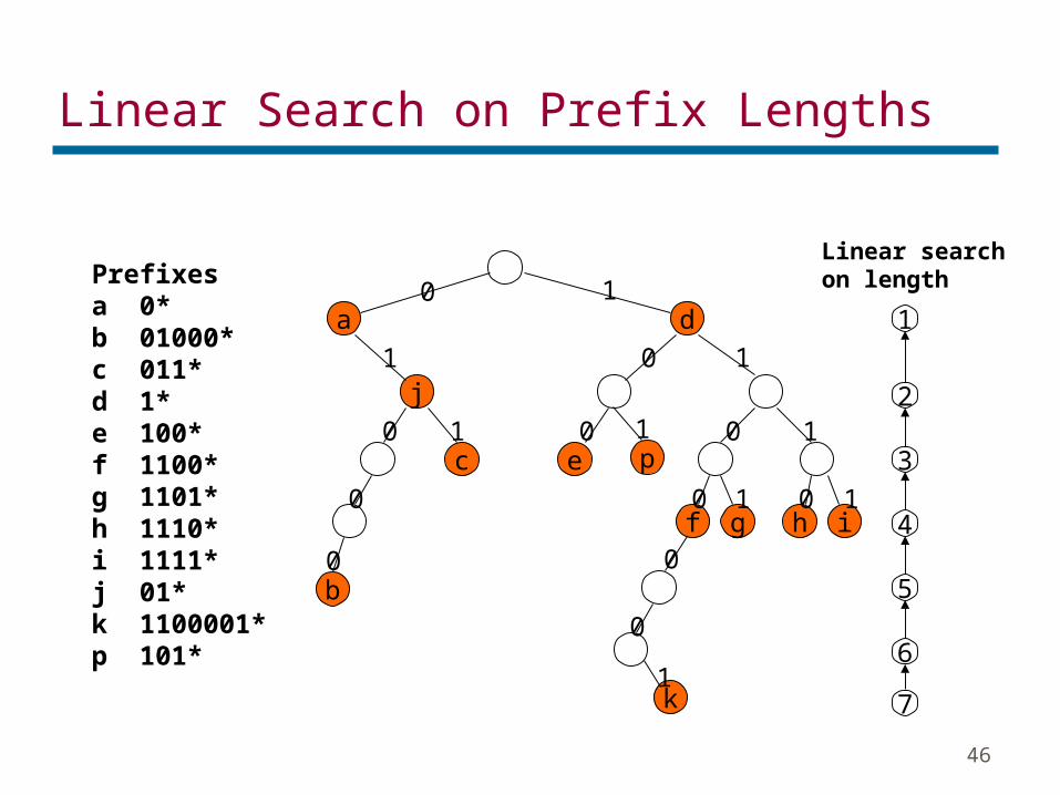
Hash-based Scheme

Store a hash table for each prefix length

Hash key is the prefix value and prefix length

Search scheme Linear search on prefix lengths Binary search on prefix lengths

Need to provide intermediate markers• Guide to more specific prefix

Need pre-computation per marker• Avoid backtracking

46

Linear Search on Prefix Lengths

Prefixesa 0*b 01000*c 011*d 1*e 100*f 1100*g 1101*h 1110*i 1111*j 01*k 1100001*p 101*

a d

j

c

b

e

h if g

0

0

0

0

0

0

0

0 0

1

1

1 1

1

11

p1

0

0

k1

1

3

2

5

7

6

4

Linear searchon length

47

Binary Search on Prefix Lengths

Prefixesa 0*b 01000*c 011*d 1*e 100*f 1100*g 1101*h 1110*i 1111*j 01*k 1100001*p 101*

a d

j

c

b

e

h if g

0

0

0

0

0

0

0

0 0

1

1

1 1

1

11

p1

0

0

k1

1

3

2

5

7

6

4

Binary search on length

48

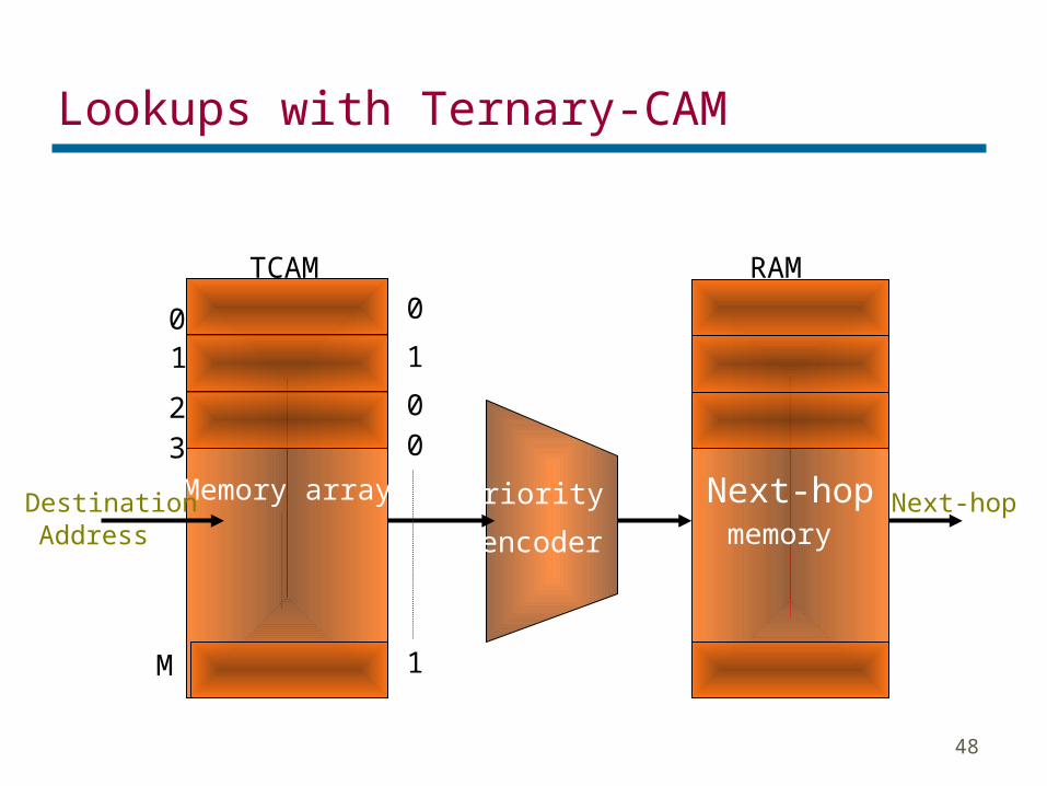
Lookups with Ternary-CAM

Memory array Priority

encoder

Next-hopmemory

Next-hop

TCAM RAM

01

23

M

0

1

00

1

DestinationAddress

49

Lookups with Ternary-CAM

Advantages Suitable for multiple

fields Fast: 16-20 ns (50-66

Mpps) Simple to understand

Disadvantages Inflexible: range-to-prefix

blowup Density: largest available in

2000 is 32K x 128 (but can be cascaded)

Management software, and on-chip logic: non-trivial complexity

Incremental updates: slow

50

MPLS

Multiple Protocol Label Switching A versatile solution to address the problems

faced by present networks such as speed, scalability, quality of service management, and traffic engineering

51

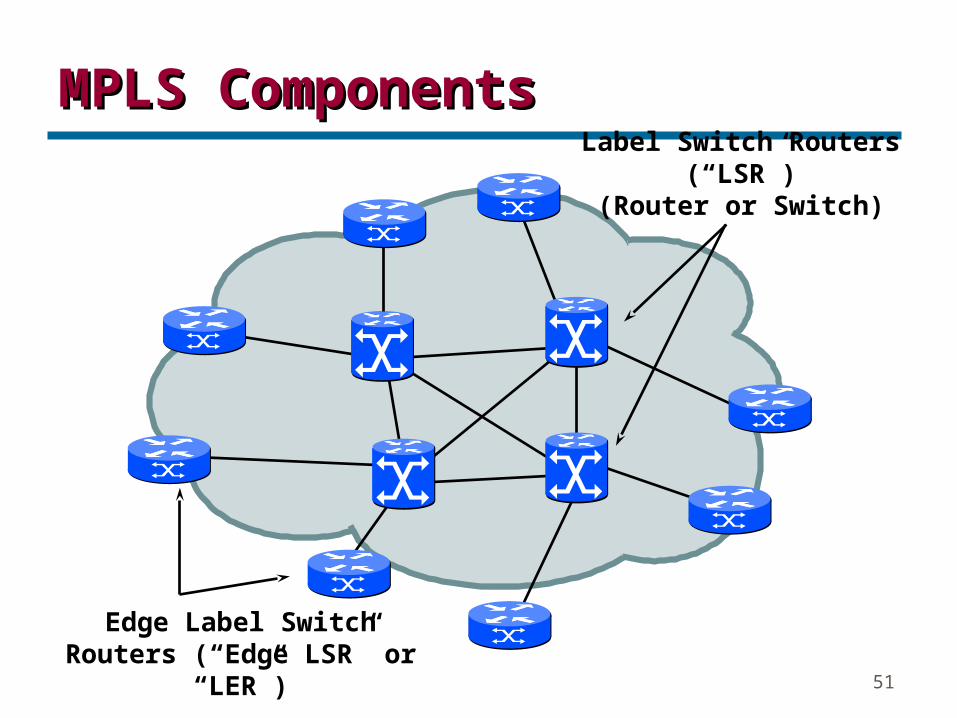
Edge Label Switch Routers (“Edge LSR” or “LER”)

Label Switch Routers(“LSR”)

(Router or Switch)

MPLS ComponentsMPLS Components

52

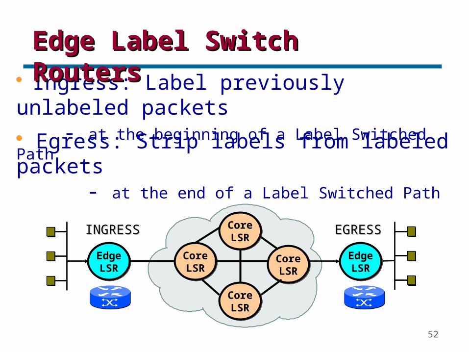
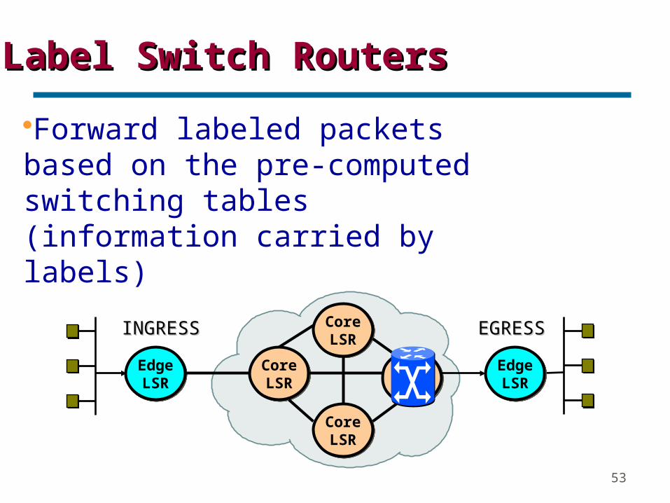
Ingress: Label previously unlabeled packets- at the beginning of a Label Switched Path

Edge Label Switch RoutersEdge Label Switch Routers

Egress: Strip labels from labeled packets- at the end of a Label Switched Path

CoreLSRCoreLSR

CoreLSRCoreLSR

CoreLSRCoreLSR

CoreLSRCoreLSR

EdgeLSR

EdgeLSR

INGRESSINGRESS

EdgeLSR

EdgeLSR

EGRESSEGRESS

53

Forward labeled packets based on the pre-computed switching tables (information carried by labels)

CoreLSRCoreLSR

CoreLSRCoreLSR

CoreLSRCoreLSR

CoreLSRCoreLSR

EdgeLSR

EdgeLSR

INGRESSINGRESS

EdgeLSR

EdgeLSR

EGRESSEGRESS

Label Switch RoutersLabel Switch Routers

54

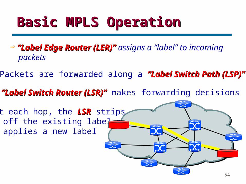
Basic MPLS OperationBasic MPLS Operation

“ “Label Edge Router (LER)”Label Edge Router (LER)” assigns a “label” to incoming packets

Packets are forwarded along a “Label Switch Path (LSP)”“Label Switch Path (LSP)”

“ “Label Switch Router (LSR)”Label Switch Router (LSR)” makes forwarding decisions

At each hop, the LSRLSR strips off the existing label and applies a new label

55

InLbl

AddressPrefix

OutI’face

OutLbl

- 128.89 1 4

- 171.69 1 5

1

1

1

0 128.89

171.69

MPLS Packet ForwardingMPLS Packet ForwardingIn

LblInI/F

AddressPrefix

OutI’face

OutLbl

4 2 128.89 0 9

8 3 128.89 0 10

5 2 171.69 1 7

InLbl

InI/F

AddressPrefix

OutI’face

OutLbl

9 1 128.89 0 -

10 1 128.89 0 -

2 0

128.89.25.4128.89.25.4

128.89.25.4128.89.25.4

128.89.25.4128.89.25.4 44

128.89.25.4128.89.25.4 99

56

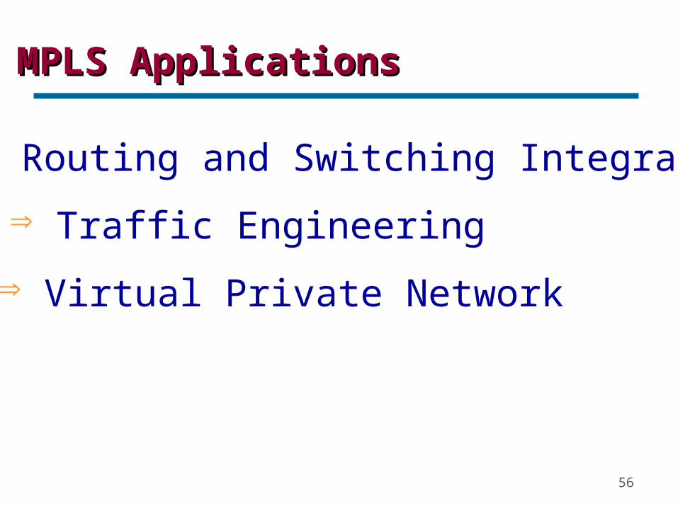
MPLS ApplicationsMPLS Applications

Routing and Switching Integration

Traffic Engineering

Virtual Private Network

57

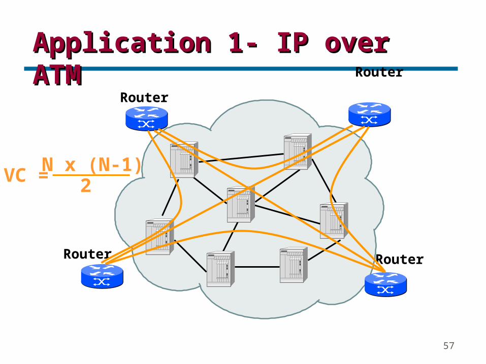
Application 1- IP over ATMApplication 1- IP over ATM

Router

Router

Router

Router

N x (N-1)2VC =

58

IP over ATM in a MPLS NetworkIP over ATM in a MPLS Network

Label Edge Router “LER”

LER LER

LER

LSR

LSR

Less Complexity and a lower cost of ownershipLess Complexity and a lower cost of ownership

59

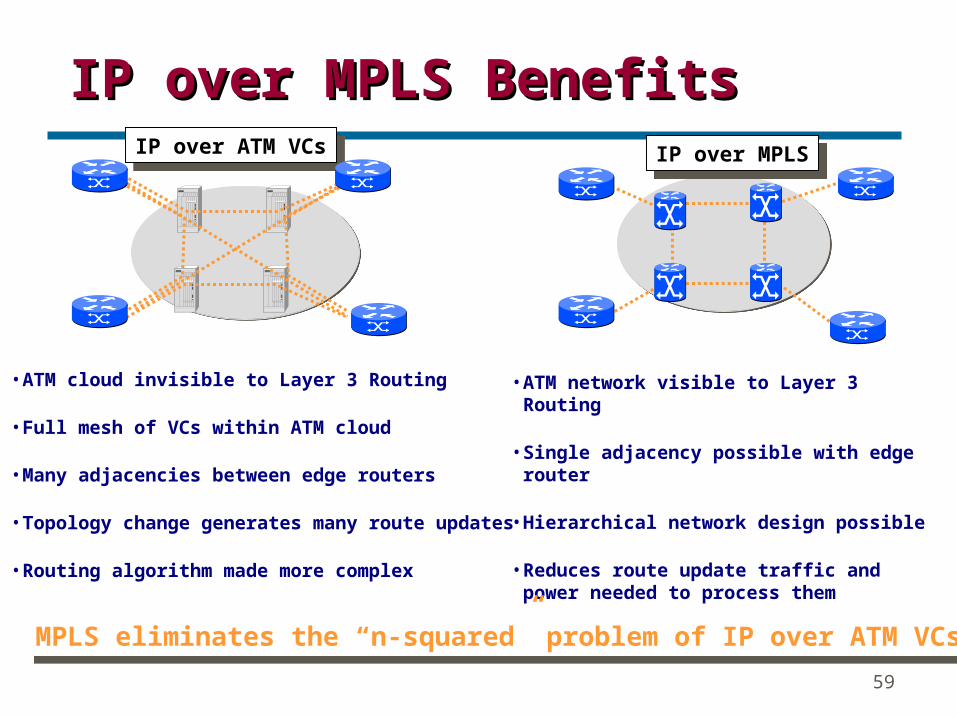
• ATM cloud invisible to Layer 3 Routing

• Full mesh of VCs within ATM cloud

• Many adjacencies between edge routers

• Topology change generates many route updates

• Routing algorithm made more complex

• ATM network visible to Layer 3 Routing

• Single adjacency possible with edge router

• Hierarchical network design possible

• Reduces route update traffic and power needed to process them

MPLS eliminates the “n-squared” problem of IP over ATM VCsMPLS eliminates the “n-squared” problem of IP over ATM VCs

IP over ATM VCsIP over ATM VCsIP over MPLSIP over MPLS

IP over MPLS BenefitsIP over MPLS Benefits

60

Application 2 - Traffic EngineeringApplication 2 - Traffic Engineering

Router

DYNAMIC ROUTINGDYNAMIC ROUTING

Router

DA 171.68.90.5DA 171.68.90.5

LAN

Network 171.68Network 171.68

61

Application 2- Traffic EngineeringApplication 2- Traffic Engineering

MPLS switch

DA 171.68.90.5DA 171.68.90.5

LAN

Network 171.68Network 171.68

LER

Label Switched PathLabel Switched Path

62

Application 3- Virtual Private NetworksApplication 3- Virtual Private Networks

VPN B Tunnel

VPN A Tunnel

VPN A/Site 2VPN A/Site 1

VPN A/Site 3

VPN B/Site 2 VPN B/Site 3

VPN B/Site 1

RA1RA2

RA3

RB2

RB1

RB3

63

MPLS Generic Label FormatMPLS Generic Label Format

Link LayerHeader

MPLSSHIM

Network LayerHeader

Other LayersHeaders and Data

Label CoS S TTL

32 bits

20 bits 3 bits 8 bits1 bit

64

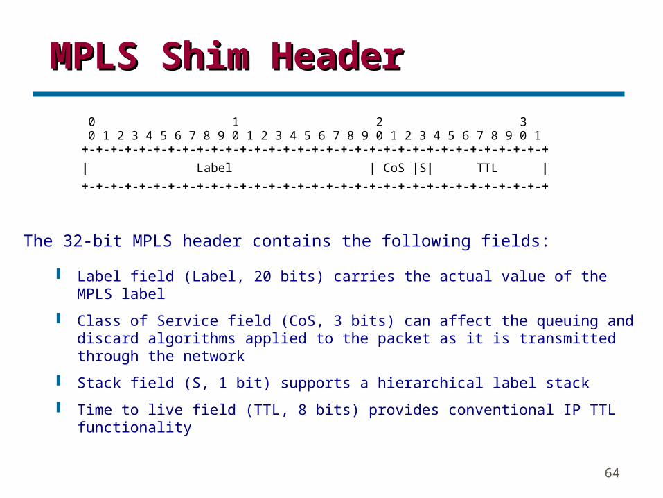
0 1 2 30 1 2 3 4 5 6 7 8 9 0 1 2 3 4 5 6 7 8 9 0 1 2 3 4 5 6 7 8 9 0 1+-+-+-+-+-+-+-+-+-+-+-+-+-+-+-+-+-+-+-+-+-+-+-+-+-+-+-+-+-+-+-+-+

+-+-+-+-+-+-+-+-+-+-+-+-+-+-+-+-+-+-+-+-+-+-+-+-+-+-+-+-+-+-+-+-+

| Label | CoS |S| TTL |

The 32-bit MPLS header contains the following fields:

Label field (Label, 20 bits) carries the actual value of the MPLS label

Class of Service field (CoS, 3 bits) can affect the queuing and discard algorithms applied to the packet as it is transmitted through the network

Stack field (S, 1 bit) supports a hierarchical label stack

Time to live field (TTL, 8 bits) provides conventional IP TTL functionality

MPLS Shim HeaderMPLS Shim Header

65

IP over Data Link LayerIP over Data Link Layer

Shim Header Layer 3 HeaderPPP Header

Label

PPP PPP HeaderHeader

LAN MAC LAN MAC HeaderHeader

Shim Header Layer 2 HeaderMAC Header

66

LabelLabel CreationCreation

Several Methods:

Topology-driven method

Control-driven method

Traffic-driven method

67

LSP is provisioned using:

Label Distribution Protocol LDP and its extension Constraint-based Routing LDP (CR-LDP)

Traffic Engineering extensions for Resource ReSerVation Protocol (RSVP-TE)

Label Distribution Protocol - LDPLabel Distribution Protocol - LDP