1 remote sensing of the ocean and atmosphere: john wilkin sea surface temperature...
TRANSCRIPT

1
Remote Sensing of the Oceanand Atmosphere:
John Wilkin
Sea SurfaceTemperature
[email protected] Building Room 214C609-630-0559

2

3

5

6

7

8

9

10

11

12

13
http://www.oso.noaa.gov/poesstatus Polar Orbiting Environmental Satellites (POES) Office of Satellite Operations

14
http://www.oso.noaa.gov/poesstatus
Polar Orbiting Environmental Satellites (POES) Office of Satellite Operations

15

16

17
All the in situ temperature observations in Australia waters since 1950

18
Ocean
Troposphere
Stratosphere
clouds
T
TS
Tb
sun glint
volcanic aerosols
tropospheric aerosols
sensor
Emitted surface radiance
upwelled atmospheric radiance
water vapor
buoy

10-12 m 3.5-4.1 m
Relative atmospheric transmission plotted vs. decreasing wavelength

10-12 m3.5-4.1 m
Relative atmospheric transmission plotted vs. increasing wavelength

21wavelength
Sensitivity of brightness to change in blackbody temperature
brightness of 300K blackbody
Brightness temperature difference due to atmosphere
3.5 μm 10 μm 12 μm

22
Wavelength bands used for IR SST imaging• Require high transmittance
(low absorption) in atmosphere (i.e. a “window”)
• Need significant emittance at black-body temperature typical of the ocean
• Preferably high sensitivity of radiance to change in SST
• Wavelengths typically used in practice:– AVHRR band 3B ~ 3.7 m
(MODIS band 20) night-time SST
– AVHRR bands 4 and 5 ~10.8 and ~12 m (MODIS 31 and 32) for day and night SST using split window algorithm

23
http://oceanworld.tamu.edu/resources/ocng_textbook/chapter06/chapter06_10.htm1 m 2 m
At 11 m, IR exitance comes from top 30 m of ocean
Absorption coefficient for pure water as a function of wavelength λ of the radiation.

24
Night time weak winds and strong winds (anytime) case
Day time weak winds case
See also Fig 7.4 in Martin
25
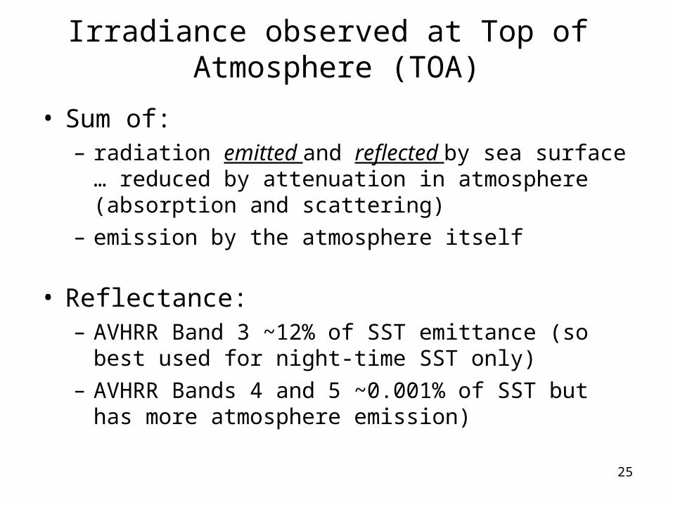
Irradiance observed at Top of Atmosphere (TOA)
• Sum of:– radiation emitted and reflected by sea surface …
reduced by attenuation in atmosphere (absorption and scattering)
– emission by the atmosphere itself
• Reflectance:– AVHRR Band 3 ~12% of SST emittance (so best
used for night-time SST only)
– AVHRR Bands 4 and 5 ~0.001% of SST but has more atmosphere emission)

26
Converting multi-channel irradiance to SST data

27
Correcting for the atmosphere

28

29

30

31

32

33
int cloud_mask(time, lat, lon) ;cloud_mask:missing_value = -999 ;cloud_mask:long_name = "Cloud_mask" ;cloud_mask:_FillValue = -999 ;cloud_mask:Convention = ”
0=passed 1=failed time test 2=failed low temp test 4=failed high gradient test 8=failed climatology test; Logical tests are summed" ;
cloud_mask:documentation = ”“A measurement fails the time test if it is more than 2 degrees cooler than the median of the satellite passes in the previous 24 hrs;\n",
"A measurement fails the low temp test if it is more than 2 standard deviations colder than any other measurement in that image;\n",
"A measurement fails the high gradient test if its temperature gradient is greater than 2 standard deviations of all gradients in the image;\n",
"A measurement fails the climatology test if the temperature is more than 5 degrees colder than the climatologies calculated by NSIPP AVHRR Pathfinder and Erosion Global 9km SST Climatology (Casey, Cornillon). A description of this climatology can be found at ftp://podaac.jpl.nasa.gov/pub/documents/dataset_docs/nsipp_climatology.htm;\n",
"If any measurement is fails a test, all neighboring measurements within 3km are also automatically failed." ;
Example: cloud flagging of data on IMCS OPeNDAP data server for the “Bigbight” region from Cape Hatteras to Nova Scotia
http://tashtego.marine.rutgers.edu:8080/thredds/cool/avhrr/catalog.xml

34

35

36

37

38
Night time weak winds and strong winds (anytime) case
Day time weak winds case
See also Fig 7.4 in Martin

39http://www.aoml.noaa.gov/phod/dac/gdp_drifter.php
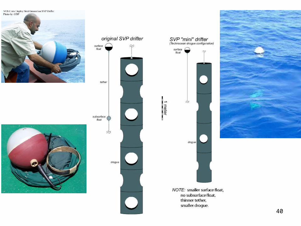
40

41

42
Global SST bias monitoring (monitored sensor minus reference sensor at the colocated points for each day):
* in solid blue, time series of the bias between the sensor raw sst (without any correction applied) and the reference sst * In green, time series of the bias between the sensor sst (with SSES correction as provided in L2 files) and the reference sst * in dashed blue, bias between the sensor adjusted sst (with SSES correction and intercalibration adjustment) and the reference * in red, bias between the adjusted sst (with SSES correction and intercalibration adjustment) and the Odyssea optimal interpolation * the histogram plots the number of sensor/reference match-ups available each day

43