Redescending M-estimators in regression analysis, clusteranalysis and image analysis

Christine Muller

Carl von Ossietzky University Oldenburg

Institute for Mathematics

Postfach 2503, D - 26111 Oldenburg, Germany

Abstract. We give a review on the properties and applications of M-estimators

with redescending score function. For regression analysis, some of these redescending

M-estimators can attain the maximum breakdown point which is possible in this setup.

Moreover, some of them are the solutions of the problem of maximizing the efficiency un-

der bounded influence function when the regression coefficient and the scale parameter are

estimated simultaneously. Hence redescending M-estimators satisfy several outlier robust-

ness properties. However, there is a problem in calculating the redescending M-estimators

in regression. While in the location-scale case, for example, the Cauchy estimator has only

one local extremum this is not the case in regression. In regression there are several local

minima reflecting several substructures in the data. This is the reason that the redescend-

ing M-estimators can be used to detect substructures in data, i.e. they can be used in

cluster analysis. If the starting point of the iteration to calculate the estimator is coming

from the substructure then the closest minimum corresponds to this substructure. This

property can be used to construct an edge and corner preserving smoother for noisy im-

ages so that there are applications in image analysis as well.

Keywords: redescending M-estimator, regression, breakdown point, optimality, cluster

analysis, image analysis, kernel estimator.

AMS Subject classification: primary 62 J 05, 62 G 35, secondary 62 H 30, 62 G 07,

62 M 40, 62 P 99.

1 Redescending M-estimators

Regard a general linear model yn = x>nβ + zn, n = 1, . . . , N , where yn ∈ < is the

observation, zn ∈ < the error, xn ∈ <p the known regressor and β ∈ <p the unknown

parameter vector. For distributional assertions, it is assumed that the errors zn are

1

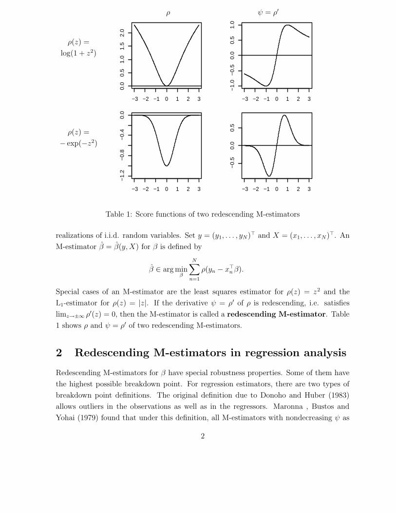
ρ ψ = ρ′

ρ(z) =

log(1 + z2)

−3 −2 −1 0 1 2 3

0.0

0.5

1.0

1.5

2.0

−3 −2 −1 0 1 2 3

−1

.0−

0.5

0.0

0.5

1.0

ρ(z) =

− exp(−z2)

−3 −2 −1 0 1 2 3

−1

.2−

0.8

−0

.40

.0

−3 −2 −1 0 1 2 3

−0

.50

.00

.5

Table 1: Score functions of two redescending M-estimators

realizations of i.i.d. random variables. Set y = (y1, . . . , yN)> and X = (x1, . . . , xN)>. An

M-estimator β = β(y,X) for β is defined by

β ∈ arg minβ

N∑

n=1

ρ(yn − x>nβ).

Special cases of an M-estimator are the least squares estimator for ρ(z) = z2 and the

L1-estimator for ρ(z) = |z|. If the derivative ψ = ρ′ of ρ is redescending, i.e. satisfies

limz→±∞ ρ′(z) = 0, then the M-estimator is called a redescending M-estimator. Table

1 shows ρ and ψ = ρ′ of two redescending M-estimators.

2 Redescending M-estimators in regression analysis

Redescending M-estimators for β have special robustness properties. Some of them have

the highest possible breakdown point. For regression estimators, there are two types of

breakdown point definitions. The original definition due to Donoho and Huber (1983)

allows outliers in the observations as well as in the regressors. Maronna , Bustos and

Yohai (1979) found that under this definition, all M-estimators with nondecreasing ψ as

2

the L1-estimator behave as bad as the least squares estimator. All these M-estimators

have a breakdown point of 1N

which means that they can be biased arbitrarily by one

outlier. He et al. (1990) and Ellis and Morgenthaler (1992) found that the situation

changes completely if outliers appear only in the observations and not in the regressors,

a situation which in particular appears in designed experiments where the regressors are

given by the experimenter. In this situation the breakdown point is defined as

ε∗(β, y,X) = min1

N

{

M ; supy∈YM (y)

‖β(y,X) − β(y,X)‖ = ∞

}

,

where

YM(y) ={

y ∈ <N ; ]{n; yn 6= yn} ≤M}

.

Using this defintion, an upper bound for the breakdown point of regression equivariant

estimators is according to Muller (1995, 1997)

ε∗(β, y,X) ≤1

N

⌊

N −N (X) − 1

2

⌋

, (1)

where N (X) is the maximum number of xn lying in a subspace of <p, i.e.

N (X) = supβ 6=0

]{n; x>nβ = 0}.

The upper bound is attained by some least trimmed squares estimators (Muller 1995,

1997) and by redescending M-estimators whose score function ρ has slow variation, i.e.

satisfies

limt→∞

ρ(tu)

ρ(t)= 1 for all u > 0 (2)

(Mizera and Muller 1999). In particular the score function of the Cauchy M-estimator

satisfies (2). This score function is shown in the first row of Table 1. Up to now it

is unclear whether the M-estimators with slowly varying score function are the only M-

estimators whose breakdown point attains the upper bound for any configuration (design)

of the regressors. For special designs also the breakdown point of other M-estimators as

of the L1-estimators can attain the upper bound (Muller 1996).

The results of Mizera and Muller (1999) were shown for known scale. However re-

descending M-estimators are very sensitive with respect to the scale parameter so that

in practice the scale parameter must be estimated simultaneously. Mizera and Muller

(2002) showed that also the breakdown point of some tuned Cauchy estimators which

simultaneously estimate the regression and the scale parameter attains the upper bound

3

(1). A M-estimator for simultaneous estimation of the regression and scale parameter is

given by

(β, σ) ∈ arg minβ,σ

N∑

n=1

ρ

(

yn − x>nβ

σ

)

+K lnσ,

where K is the tuning constant. The estimator is called untuned if K = N . Mizera and

Muller showed their result only for the Cauchy M-estimator although it seems plausible

that it holds also for other M-estimators. The high breakdown point behavior of the

Cauchy M-estimator was also found by He et al. (2000) who compared the behaviour

of t-type M-estimators with respect to the original definition of the breakdown point of

Donoho and Huber (1983). However the situation changes completely when orthogonal

regression in an errors-in-variables model is considered. Then according to Zamar (1989),

any M-estimator with unbounded score function ρ has asymptotically a breakdown point

of zero. In particular the Cauchy M-estimator for orthogonal regression has an asymptotic

breakdown point of zero.

But redescending M-estimators are not only good with respect to the breakdown point

but have also some optimality properties with respect to efficiency under bounded influ-

ence function. This can be shown by extending the class of M-estimators to estimators

given by

(β, σ) ∈ arg minβ,σ

N∑

n=1

ρ

(

yn − x>nβ

σ, xn

)

+N ln σ

or more general to estimators (β, σ) which are given as solutions of

N∑

n=1

ψ

(

yn − x>nβ

σ, xn

)

x>n = 0 (3)

N∑

n=1

(

1 − ψ

(

yn − x>nβ

σ, xn

)

yn − x>nβ

σ

)

= 0. (4)

Under suitable regularity conditions, the asymptotic covariance matrix of these estimators

is (see Hampel et al. 1986)

σ2

(

Vβ(ψ, δ) 0

0 Vσ(ψ, δ)

)

,

where

Vβ(ψ, δ) = I(δ)−1 Qβ(ψ, δ) I(δ)−1

4

and

Vσ(ψ, δ) = Qσ(ψ, δ)/Mσ(ψ, δ)2

with

I(δ) =

∫

xx> δ(dx),

Mσ(ψ, δ) =

∫

(z ψ(z, x) − 1) (z2 − 1)P (dz) δ(dx),

Qβ(ψ, δ) =

∫

ψ(z, x)2 xx> P (dz) δ(dx),

Qσ(ψ, δ) =

∫

(z ψ(z, x) − 1)2 P (dz) δ(dx).

Thereby δ denotes the asymptotic design measure. The influence function of the M

estimator is (see Hampel et al. 1986)

(

IFβ(z, x, ψ, δ)

IFσ(z, x, ψ, δ)

)

,

where

IFβ(z, x, ψ, δ) = I(δ)−1 xψ(z, x)

and

IFσ(z, x, ψ, δ) := (z ψ(z, x) − 1)/Mσ(ψ, δ).

For estimation of only the regression parameter the most efficient M-estimators with

bounded influence function are solutions of minimizing trVβ(ψ, δ) under the side condi-

tion supz,x |IFβ(z, x, ψ, δ)| ≤ bβ. These solutions were characterized by Hampel (1978),

Krasker (1980), Bickel (1981, 1984), Huber (1983), Rieder (1987, 1994), Kurotschka and

Muller (1992) and Muller (1994, 1997) and are given by nondecreasing score functions

ψ. For simultaneous estimation of the regression and scale parameter, the most efficient

estimators with bounded influence function have score functions ψ which simultaneously

minimize

trVβ(ψ, δ) and Vσ(ψ, δ)

under the side conditions that

supz,x

|IFβ(z, x, ψ, δ)| ≤ bβ and supz,x

|IFσ(z, x, ψ, δ)| ≤ bσ.

5

It is not easy to give a complete characterization of these score functions. But the results

of Bednarski and Muller (2001) for the location-scale case indicate that the optimal score

functions are given by

ψ(z, xn) = a(xn)/z for |z| > c(xn),

where a(xn) and c(xn) are quantities depending on the regressors. This means that the

optimal M-estimators are redescending M-estimators. The corresponding score function

ρ of the form ρ(z, x) = a(x) log(z) is slowly varying in the sense of (2). Although the

score functions ρ differ by its dependence on the regressors x from the score functions

considered in Mizera and Muller (1999), the result of Mizera and Muller is still valid.

This can be seen by simply extending their proof to the general type of score functions

which is possible since the regressors are fixed without outliers. Hence the most efficient

M-estimators with bounded influence function have also a breakdown point which attains

the upper bound (1) for breakdown points.

The main problem with the most efficient M-estimators with bounded influence func-

tion and highest breakdown point is their computation. Because of the redescending

form of the score function, the objective function has several local minima in the general

case and thus there are several simultaneous solutions of (3) and (4). One exception is

the Cauchy estimator for location and scale where only one local extremum exists if the

distribution is not concentrated with equal probabilities at two points (see Copas 1975).

However, Cauchy estimators for regression already have the general problem of several

local extrema as Gabrielsen (1982) pointed out. But highest breakdown point and even

consistency can be only achieved if the global minimum of the objective function is used.

In the location case, the global minimum is often the symmetry center of the underlying

distribution so that the global minimum can be found with Newton-Raphson method

starting at a consistent estimator for the symmetry center (Andrews et al. 1972, Collins

1976, Clarke 1983, 1986). However for asymmetric distributions or regression the situ-

ation is more complicated (see Freedman and Diaconis 1982, Jureckova and Sen 1996,

Mizera 1994, 1996). One possibility of finding the global minimum is to calculate each

local minimum. For smooth score functions like that of the Cauchy M-estimator for re-

gression this can be done by Newton-Raphson method starting at any hyperplane through

p points of the data set. An alternative method is the EM-algorithm proposed by Lange

et al. (1989) for computing regression estimators with t-distributed errors.

6

3 Redescending M-estimators in cluster analysis

The disadvantage of redescending M-estimators that their objective function has several

local minima becomes an advantage in cluster analysis. Morgenthaler (1990) already

pointed out that each local minimum corresponds to a substructure of the data and

Hennig (2000, 2003) used a fixed point approach based on redescending M-estimators

for clustering. However the use of redescending M-estimators in cluster analysis has

the problem that local minima do not correspond only to hyperplanes (lines in simple

regression) which can be viewed as cluster centers. Local minima can also correspond to

hyperplanes orthogonal to hyperplanes given by clusters or, more general, to hyperplanes

fitting several clusters or even all clusters. Arslan (2003) even found that the smallest

local minimum often correspond to the over all fit. She therefore developed a test for

detecting the ”right” local minima, i.e. those minima which correspond to regression

clusters.

The problem of finding the ”right” local minima can be facilitated by using more

extreme redescending M-estimators and small scale parameters. For example the score

function of the second line of Table 1, i.e.

ρ(z) = − exp(−z2) (5)

can be used which is up to a constant the density of the normal distribution. M-estimators

based on such a score function cannot be interpreted anymore as maximum likelihood

estimators as it is the case for the Cauchy M-estimator. The score function is also not

anymore slowly varying in the sense of (2). But the integral of the score function is finite

which is not the case for the other M-estimators which can be interpreted as maximum

likelihood estimators. The property of a finite integral leads to a relation of M-estimators

to kernel density estimators, an observation recently used also by Chen and Meer (2002).

For that note that minimization of

N∑

n=1

ρ

(

yn − x>nβ

sN

)

is equivalent to maximization of

hN(β) = −1

N

N∑

n=1

1

sN

ρ

(

yn − x>nβ

sN

)

. (6)

Here sN denotes a given scale parameter depending on the sample sizeN . In the context of

kernel density estimation, the parameter sN plays the role of the bandwidth. In particular

7

for the location case, where xn = 1 for all n = 1, . . . , N , we have the well known kernel

density estimator

fN(µ) = −1

N

N∑

n=1

1

sN

ρ

(

yn − µ

sN

)

.

It is also known (see e.g. Silverman 1986) that the kernel density estimator f(µ) satisfies

limN→∞

fN(µ) = f(µ) (7)

with probability 1 if∫

−ρ(z) dz = 1, sN converges to zero and some additional regularity

conditions are satisfied. If the observations are coming from different location clusters,

their common distribution has a density with several local maxima. The points of the

local maxima can be interpreted as the true cluster centers. Hence the convergence (7)

implies the convergence of the local maximum points of fN to the local maximum points

of f and thus to the true cluster centers. This holds of course under some regularity

conditions.

This reasoning can be used also for regression clusters as Muller and Garlipp (2002)

pointed out. Muller and Garlipp proved that, like fN , also hN of (6) converges to a

limit function h if∫

−ρ(z) dz = 1, sN converges to zero and some regularity conditions

are satisfied. Examples showed that the highest local maxima of this limit function h

correspond to real regression clusters. However there are also other local maxima with

no relation to a real regression cluster, but these are much smaller so that they can be

distinguished from the other. Because of the convergence of hN to h it can be expected

that the highest local maxima of hN correspond to real clusters and that they can be

found by studying the height of the local maxima. Muller and Garlipp showed also that

the same reasoning holds for orthogonal regression in an errors-in-variables model by

maximizing

hN(a, b) = −1

N

N∑

n=1

1

sN

ρ

(

(yn, x>n )a− b

sN

)

with respect to a ∈ <p+1 with ‖a‖ = 1 and b ∈ <. Besides the rotation invariance, the

orthogonal regression has the advantage that the limit function h has an interpretation as

density. How regression clusters can be found by this method is demonstrated by Figures

2 and 3. For more explanations of this application, see the next section.

4 Redescending M-estimators in image analysis

We will consider here two problems of image analysis. One problem is to detect objects

and structures in the image. The other problem is to reconstruct a noisy image.

8

1 20 40 60 80 100

120

4060

8010

0

Figure 1: Noisy Image

0 20 40 60 80

020

4060

80

Figure 2: Edge Points

0 20 40 60 80

020

4060

80

1

2

3

4 5 6 7

Figure 3: Regression Lines

2 1 3 7 6 5 4

050

100

150

200

250

225 224219

109 105 102 102

Figure 4: Heights of Maxima

For detecting objects and structures a widely used method in computer vision are the

Hough transform and the RANSAC method. Both methods can be interpreted as an

M-estimator based on the zero-one score function

ρ(z) =

{

0 if |z| ≤ 1

1 if |z| > 1.

Recent development used also a smoothed version of the zero-one function or the biweight

function

ρ(z) =

{

1 − (1 − z2)3 if |z| ≤ 1

1 if |z| > 1.

See e.g. Chen et al. (2001) for an overview. The methods mainly differ in the choice

of the scale parameter and how the local maxima/minima are found which correspond

to substructures/clusters. The methods of finding the right maxima/minima are always

as that of Chen et al. (2001) rather complicated. However Muller and Garlipp (2002)

9

demonstrated for the problem of finding the edges of a triangle that the local maxima

corresponding to the edge lines can be easily found by the height of the local maxima.

They used the negative of the score function given by (5) which is differentiable so that

the Newton-Raphson method can be easily applied for determining the local maxima. It

turned out that the result does not depend very much on the scale parameter. Moreover,

there is a natural choice of the scale parameter since, in a first step, points are determined

which should lie close to the edges. These points can be found by using a rotational density

kernel estimator, a method proposed by Qiu, P. (1997). The bandwidth of the rotational

density kernel estimator is the natural choice of the scale parameter. In the Figures 1 to 4

this method is demonstrated. Thereby, Figure 2 shows the points close to edges found by

the method of Qiu and Figure 3 provides the regression lines found by the cluster method.

Figure 4 shows that the three right regression lines 1, 2, 3 have significantly larger heights

of the local maxima.

For finding all local maxima/minima, the Newton-Raphson method starts at all hyper-

planes given by p data points, in the two-dimensional case at all lines given by two points.

Often the found local maximum corresponds to a cluster to which the starting hyperplane

belongs to. This is even always the case for the location case (p = 1, xn = 1). This

observation can be used for image denoising as Chu et al. (1998) proposed. If yn = y(vn)

n = 1, . . . , N are the pixel values of the noisy image at pixel positions vn = (un, tn) lying

in [0, 1]2 then a reconstructed pixel value y(v0) at position v0 can be determined by M-

kernel estimators for nonparametric regression introduced by Hardle and Gasser (1984),

i.e. by

y(v0) = µv0= arg min

µ

N∑

n=1

1

λ2N

K

(

vn − v0

λN

)

1

sN

ρ

(

yn − µ

sN

)

,

where K is the kernel function and λN the bandwidth. As long as ρ is convex and thus ρ′

not redescending, edges are smoothed. For edge preserving image denoising, Muller (1999,

2002b) proposed kernel estimators based on high breakdown point regression estimators.

Chu et al. (1998) proposed M-kernel estimators with score function given by (5). But

the most important feature of the proposal of Chu et al. was to use as starting point

for the Newton-Raphson method the value y(v0), i.e. the pixel value in the center of

the window. This starting point ensures the edge preserving property of the estimator.

This estimator is even corner preserving as Hillebrand (2002) showed. He also showed

consistency not only for smooth areas but also for corners. A consistency proof for jump

points in the one-dimensional case can be found in Hillebrand and Muller (2002) as well

and for more general situations in Muller (2002a). Figure 7 shows how the corners and

edges are preserved by applying the method of Chu et al. on the noisy image in Figure 6.

10

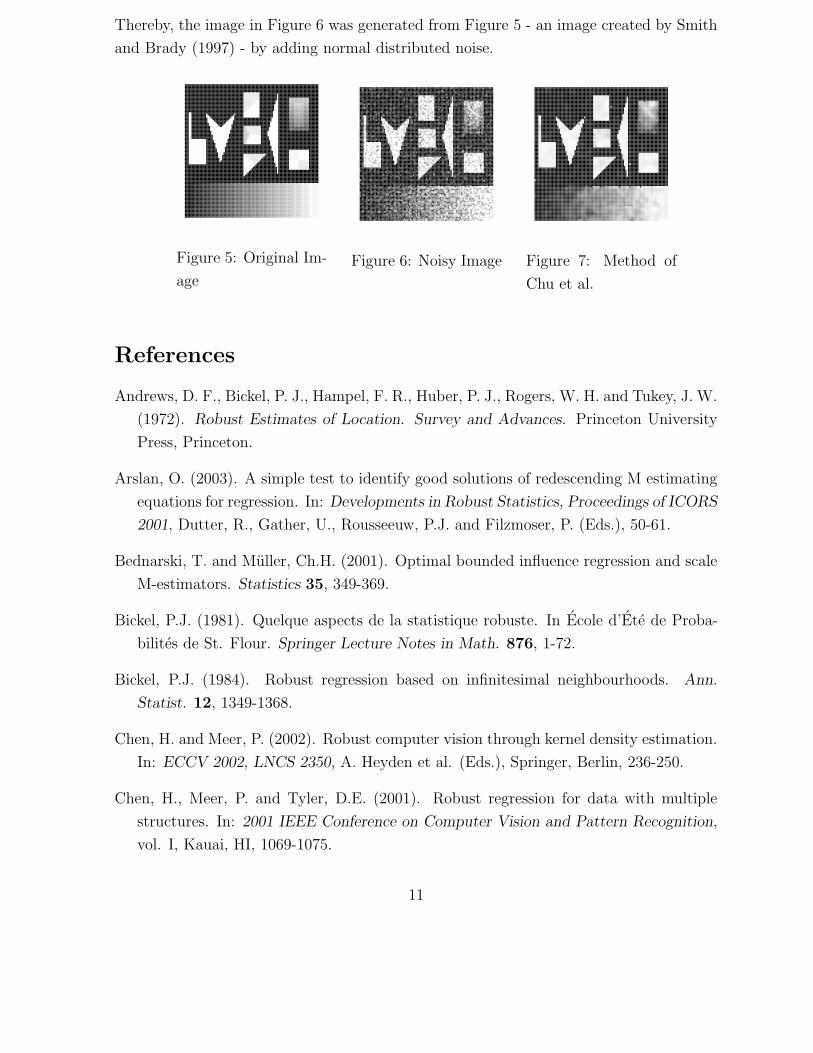
Thereby, the image in Figure 6 was generated from Figure 5 - an image created by Smith

and Brady (1997) - by adding normal distributed noise.

Figure 5: Original Im-

age

Figure 6: Noisy Image Figure 7: Method of

Chu et al.

References

Andrews, D. F., Bickel, P. J., Hampel, F. R., Huber, P. J., Rogers, W. H. and Tukey, J. W.

(1972). Robust Estimates of Location. Survey and Advances. Princeton University

Press, Princeton.

Arslan, O. (2003). A simple test to identify good solutions of redescending M estimating

equations for regression. In: Developments in Robust Statistics, Proceedings of ICORS

2001, Dutter, R., Gather, U., Rousseeuw, P.J. and Filzmoser, P. (Eds.), 50-61.

Bednarski, T. and Muller, Ch.H. (2001). Optimal bounded influence regression and scale

M-estimators. Statistics 35, 349-369.

Bickel, P.J. (1981). Quelque aspects de la statistique robuste. In Ecole d’Ete de Proba-

bilites de St. Flour. Springer Lecture Notes in Math. 876, 1-72.

Bickel, P.J. (1984). Robust regression based on infinitesimal neighbourhoods. Ann.

Statist. 12, 1349-1368.

Chen, H. and Meer, P. (2002). Robust computer vision through kernel density estimation.

In: ECCV 2002, LNCS 2350, A. Heyden et al. (Eds.), Springer, Berlin, 236-250.

Chen, H., Meer, P. and Tyler, D.E. (2001). Robust regression for data with multiple

structures. In: 2001 IEEE Conference on Computer Vision and Pattern Recognition,

vol. I, Kauai, HI, 1069-1075.

11

Chu, C. K., Glad, I. K., Godtliebsen, F., Marron, J. S. (1998). Edge-preserving smoothers

for image processing. J. Amer. Statist. Assoc. 93, 526-541.

Clarke, B. R. (1983). Uniqueness and Frechet differentiability of functional solutions to

maximum likelihood type equations. Ann. Statist. 4, 1196-1205.

Clarke, B.R. (1986). Asymptotic theory for description of regions in which Newton-

Raphson iterations converge to location M-estimators. J. Statist. Plann. Inference

15, 71-85.

Collins, J. R. (1976). Robust estimation of a location parameter in the presence of

asymmetry. Ann. Statist. 4, 68-85.

Copas, J.B. (1975). On the unimodality of the likelihood for the Cauchy distribution.

Biometrika 62, 701-704.

Donoho, D.L. and Huber, P.J. (1983). The notion of breakdown point. In: P.J. Bickel,

K.A. Doksum and J.L. Hodges, Jr., Eds., A Festschrift for Erich L. Lehmann, Wadsworth,

Belmont, CA, 157-184.

Ellis, S. P. and Morgenthaler, S. (1992). Leverage and breakdown in L1 regression. J.

Amer. Statist. Assoc. 87, 143–148.

Freedman, D. A., and Diaconis, P. (1982). On inconsistent M-estimators. Ann. Statist.

10, 454-461.

Gabrielsen, G. (1982). On the unimodality of the likelihood for the Cauchy distribution:

Some comments. Biometrika 69, 677-678.

Hampel, F.R. (1978). Optimally bounding the gross-error-sensitivity and the influence of

position in factor space. Proceedings of the ASA Statistical Computing Section, ASA,

Washington, D.C., 59-64.

Hampel, F.R., Ronchetti, E.M., Rousseeuw, P.J. and Stahel, W.A. (1986). Robust Statis-

tics - The Approach Based on Influence Functions. John Wiley, New York.

Hardle, W. and Gasser, T. (1984). Robust nonparametric function fitting. J. R. Statist.

Soc. B 46, 42-51.

He, X., Jureckova, J., Koenker, R. and Portnoy, S. (1990). Tail behavior of regression

estimators and their breakdown points. Econometrica 58, 1195–1214.

12

He, X., Simpson, D.G. and Wang, G. (2000). Breakdown points of t-type regression

estimators. Biometrika 87, 675-687.

Hennig, C. (2000). Regression fixed point clusters: motivation, consistency and simula-

tions. Preprint 2000-02, Universitat Hamburg, Fachbereich Mathematik.

Hennig, C. (2003). Clusters, outliers, and regression: Fixed point clusters. Journal of

Multivariate Analysis. 86/1, 183-212.

Hillebrand, M. (2002). On robust corner-preserving smoothing in image processing. Ph.D.

thesis at the Carl von Ossietzky University Oldenburg, Germany.

Hillebrand, M. and Ch.H. Muller (2002). On consistency of redescending M-kernel smoothers.

Submitted.

Huber, P.J. (1983). Minimax aspects of bounded-influence regression (with discussion).

J. Amer. Statist. Assoc. 78, 66-80.

Jureckova, J., and Sen, P. K. (1996). Robust Statistical Procedures. Asymptotics and

Interrelations. Wiley, New York.

Krasker, W.S. (1980). Estimation in linear regression models with disparate data points.

Econometrica 48, 1333-1346.

Kurotschka, V. and Muller, Ch.H. (1992). Optimum robust estimation of linear aspects

in conditionally contaminated linear models. Ann. Statist. 20, 331-350.

Lange, K. L., Little R. J. A. and Taylor, J. M. G. (1989). Robust statistical modeling

using the t distribution. J. Amer. Statist. Assoc. 84 881–896.

Maronna, R. A., Bustos, O. H. and Yohai, V. J. (1979). Bias- and efficiency-robustness of

general M-estimators for regression with random carriers. In Smoothing Techniques

for Curve Estimation (T. Gasser and M. Rosenblatt, eds.) 91–116. Lecture Notes in

Mathematics 757, Springer, Berlin.

Mizera, I. (1994). On consistent M-estimators: tuning constants, unimodality and break-

down. Kybernetika 30, 289-300.

Mizera, I. (1996). Weak continuity of redescending M-estimators of location with an

unbounded objective function. Tatra Mountains Math. Publ. 7, 343-347.

Mizera, I. and Muller, Ch.H. (1999). Breakdown points and variation exponents of robust

M-estimators in linear models. Ann. Statist. 27, 1164-1177.

13

Mizera, I. and Ch.H. Muller (2002). Breakdown points of Cauchy regression-scale esti-

mators. Stat. & Prob. Letters 57, 79-89.

Morgenthaler, S. (1990). Fitting redescending M-estimators in regression. In: Robust

Regression, Lawrence, H. D. and Arthur, S. (Eds.), Dekker, New York, 105-128.

Muller, Ch.H. (1994). Optimal designs for robust estimation in conditionally contami-

nated linear models. J. Statist. Plann. Inference. 38, 125-140.

Muller, Ch.H. (1995). Breakdown points for designed experiments. J. Statist. Plann.

Inference. 45, 413-427.

Muller, Ch.H. (1996). Optimal breakdown point maximizing designs. Tatra Mountains

Math. Publ. 7, 79-85.

Muller, C.H. (1997). Robust Planning and Analysis of Experiments. Lecture Notes in

Statistics 124, Springer, New York.

Muller, Ch.H. (1999). On the use of high breakdown point estimators in the image

analysis. Tatra Mountains Math. Publ. 17, 283-293.

Muller, Ch.H. (2002a). Robust estimators for estimating discontinuous functions. Metrika

55, 99-109.

Muller, Ch.H. (2002b). Comparison of high-breakdown-point estimators for image de-

noising. Allg. Stat. Archiv 86, 307-321.

Muller, Ch.H. and T. Garlipp (2002). Simple consistent cluster methods based on re-

descending M-estimators with an application to edge identification in images. To

appear in Journal of Multivariate Analysis.

Qiu, P. (1997). Nonparametric estimation of jump surface. The Indian Journal of Statis-

tics 59, Series A, 268-294.

Rieder, H. (1987). Robust regression estimators and their least favorable contamination

curves. Stat. Decis. 5, 307-336.

Rieder, H. (1994). Robust Asymptotic Statistics, Springer, New York.

Silverman, B. W. (1986). Density Estimation for Statistics and Data Analysis. Chapman

and Hall, London.

14

Smith, S. and Brady, J. (1997). SUSAN - a new approach to low level image processing.

International Journal of Computer Vision, 23, 45-78.

Zamar, R. H. (1989). Robust estimation in the errors-in-variables model. Biometrika 76,

149-160.

15