1 radar basic - part ii
TRANSCRIPT

RADAR BasicsPart II
SOLO HERMELIN
Updated: 27.01.09Run This
http://www.solohermelin.com

Table of Content
SOLO Radar Basics
Basic Radar Concepts
The Physics of Radio Waves Maxwell’s Equations:Properties of Electro-Magnetic WavesPolarizationEnergy and MomentumThe Electromagnetic Spectrum
Introduction to Radars
Dipole Antenna Radiation
Interaction of Electromagnetic Waves with Material Absorption and Emission Reflection and Refraction at a Boundary Interface DiffractionAtmospheric Effects
RADAR BASICS - I

Table of Content (continue – 1)
SOLO Radar Basics
Basic Radar Measurements
Radar Configurations
Range & Doppler Measurements in RADAR Systems
Waveform Hierarchy
Fourier Transform of a Signal
Continuous Wave Radar (CW Radar)
Basic CW Radar
Frequency Modulated Continuous Wave (FMCW)
Linear Sawtooth Frequency Modulated Continuous Wave
Linear Triangular Frequency Modulated Continuous Wave
Sinusoidal Frequency Modulated Continuous Wave
Multiple Frequency CW Radar (MFCW)
Phase Modulated Continuous Wave (PMCW)
RADAR BASICS - I

Table of Content (continue – 2)
SOLO Radar Basics
Non-Coherent Pulse Radar
Pulse Radars
Coherent Pulse-Doppler Radar
Range & Doppler Measurements in Pulse-Radar SystemsRange Measurements
Range Measurement Unambiguity
Doppler Frequency Shift
Resolving Doppler Measurement Ambiguity
ResolutionDoppler Resolution
Angle Resolution
Range Resolution
RADAR BASICS - I

Table of Content (continue – 3)
SOLO Radar Basics
Pulse Compression WaveformsLinear FM Modulated Pulse (Chirp)
Phase Coding
Poly-Phase Codes
Bi-Phase Codes
Frank Codes
Pseudo-Random Codes
Stepped Frequency Waveform (SFWF)
RADAR BASICS - I
Table of Content (continue – 4)
SOLO Radar Basics
RF Section of a Generic Radar
Antenna
Antenna Gain, Aperture and Beam Angle
Mechanically/Electrically Scanned Antenna (MSA/ESA)
Mechanically Scanned Antenna (MSA)
Conical Scan Angular Measurement
Monopulse Antenna
Electronically Scanned Array (ESA)
RADAR BASICS - I

Table of Content (continue – 5)
SOLO Radar Basics
RF Section of a Generic Radar
Transmitters
Types of Power Sources
Grid Pulsed Tube
Magnetron
Solid-State Oscillators
Crossed-Field amplifiers (CFA)
Traveling-Wave Tubes (TWT)
Klystrons
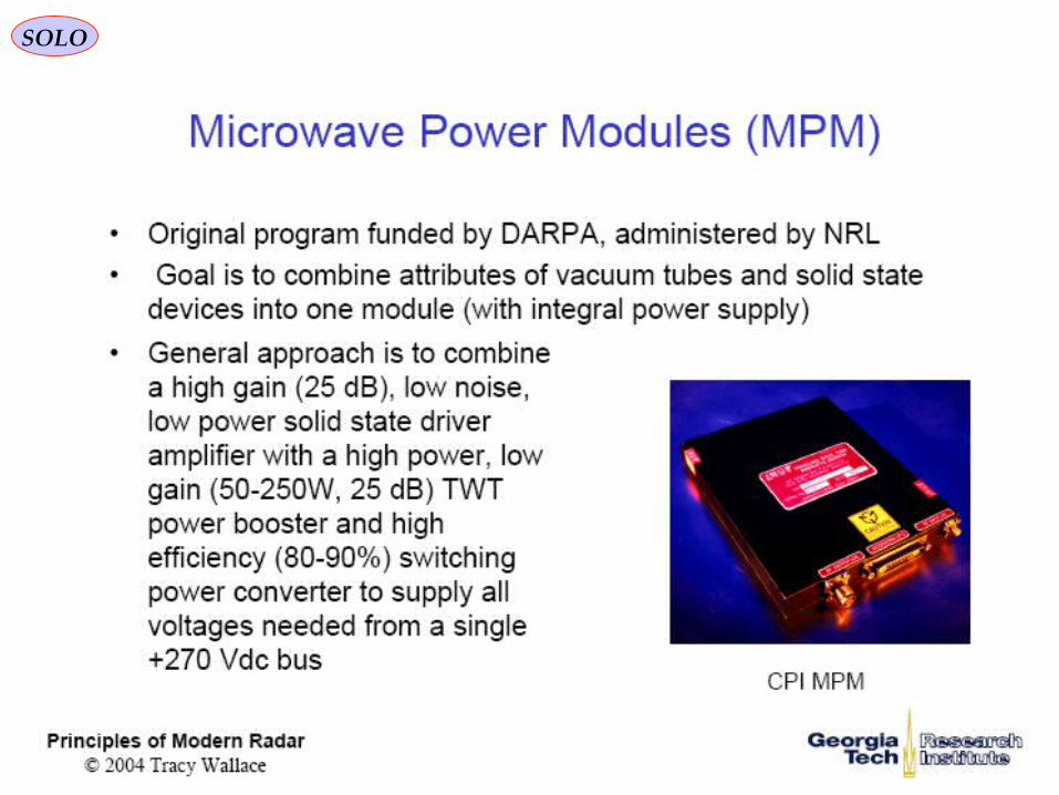
Microwave Power Modules (MPM)
Transmitter/Receiver (T/R) Modules
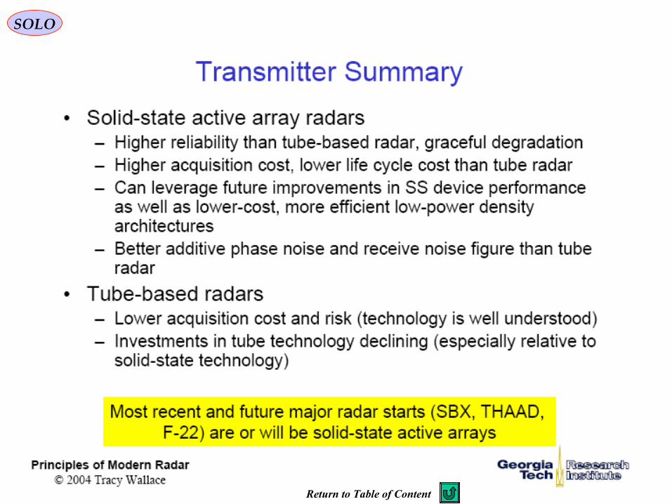
Transmitter Summary

Table of Content (continue – 6)
SOLO Radar Basics
RF Section of a Generic Radar
Radar Receiver
Isolators/CirculatorsFerrite circulators
Branch- Duplexer
TR-Tubes
Balanced Duplexer
Wave Guides
Receiver Equivalent Noise
Receiver Intermediate Frequency (IF)Mixer Technology
Coherent Pulse-RADAR Seeker Block Diagram

Table of Content (continue – 7)
SOLO Radar Basics
Radar Equation
Radar Cross Section
Irradiation
Decibels
Clutter
Ground Clutter
Volume Clutter
Multipath Return
Electronic Counter Measures (ECM)

Table of Content (continue – 8)
SOLO Radar Basics
Signal Processing
Binary Detection
Decision/Detection Theory
Radar Technologies & Applications
Radar Operation Modes
References
Continue fromRadar Basic – Part I
SOLO Radar Basics

SOLOTRANSMITTERS
Return to Table of Content

SOLO
Electron Tubesfor RF
and Microwaves
MicrowaveTubes
Low Frequency(Gridded Tubes)
Linear BeamTubes
Crossed FieldTubes
Triode
Pentode
Tetrode
TWT Hybrid(Twystron)
Klystron Magnetron
CFA
Carcinstron(MBWD)
Sivan, L., “Microwave Tube Transmitters”, Chapman & Hall, 1994, pg. 4
Transmitters

SOLO

SOLO

SOLO

SOLO

SOLO
Return to Table of Content

SOLO
Return to Table of Content

SOLO

SOLO

SOLO
Return to Table of Content

SOLO
Return to Table of Content

SOLO

In 1921 Albert Wallace Hull invented the magnetron as a powerful microwawe tube.
resonant cavities anode
catode
Filamentleads
Fig. Cutaway view of a Magnetron
pickup loop
a) slot- typeb) vane- typec) rising sun- typed) hole-and-slot- type
Figure 3: forms of the plate of magnetrons
Albert Wallace Hull (1880 – 1966)
Magnetron

Figure 1: the electron path under theinfluence of the varying magnetic field.
1. Phase: Production and acceleration of an electron beam
2. Phase: velocity-modulation of the electron beam
Figure 2: The high-frequency electrical field
3. Phase: Forming of a „Space-Charge Wheel”
Figure 3: Rotating space-chargewheel in an eight-cavity magnetron
4. Phase: Giving up energy to the ac field
Figure 4: Path of an electron
Magnetron

Magnetron tuning
A tunable magnetron permits the system to be operated at a precise frequency anywhere within a band of frequencies, as determined by magnetron characteristics. The resonant frequency of a magnetron may be changed by varying the inductance or capacitance of the resonant cavities.
inductivetuningelements
Tuner frame
anode block
Figure 12: Inductive magnetron tuning

Figure 13: Magnetron M5114B of the ATC-radar ASR-910
Figure 13: Magnetron VMX1090 of the ATC-radar PAR-80 This magnetron is even equipped with the permanent magnets necessary for the work.
Magnetron
Return to Table of Content

SOLO
Return to Table of Content

SOLO

SOLO
The Crossed-Field Amplifier (CFA), is a broadband microwave amplifier that can also be used as an oscillator (Stabilotron). The CFA is similar in operation to the magnetron and is capable of providing relatively large amounts of power with high efficiency. The bandwidth of the cfa, at any given instant, is approximately plus or minus 5 percent of the rated center frequency. Any incoming signals within this bandwidth are amplified. Peak power levels of many megawatts and average power levels of tens of kilowatts average are, with efficiency ratings in excess of 70 percent, possible with crossed-field amplifiers.
Crossed-Field Amplifier (CFA)
Also other names are used for the Crossed-Field Amplifier in the literature. • Platinotron • Amplitron • Stabilotron
Figure 2: schematically view of a Crossed-Field Amplifier (1) cathode (2) anode with resonant-cavities (3) „Space-Charge Wheel” (4) delaying strapping rings
Figure 1: water-cooled Crossed-Field Amplifier L-4756A in its transport case

SOLO
Crossed-Field Amplifier (CFA)
Because of the desirable characteristics of wide bandwidth, high efficiency, and the ability to handle large amounts of power, the CFA is used in many applications in microwave electronic systems. When used as the intermediate or final stage in high-power radar systems, all of the advantages of the CFA are used.
The amplifiers in this type of power-amplifier transmitter must be broad-band microwave amplifiers that amplify the input signals without frequency distortion. Typically, the first stage and the second stage are traveling-wave tubes (TWT) and the final stage is a crossed-field amplifier. Recent technological advances in the field of solid-state microwave amplifiers have produced solid-state amplifiers with enough output power to be used as the first stage in some systems. Transmitters with more than three stages usually use crossed-field amplifiers in the third and any additional stages. Both traveling-wave tubes and crossed-field amplifiers have a very flat amplification response over a relatively wide frequency range.
Crossed-field amplifiers have another advantage when used as the final stages of a transmitter; that is, the design of the crossed-field amplifier allows rf energy to pass through the tube virtually unaffected when the tube is not pulsed. When no pulse is present, the tube acts as a section of waveguide. Therefore, if less than maximum output power is desired, the final and preceding cross-field amplifier stages can be shut off as needed. This feature also allows a transmitter to operate at reduced power, even when the final crossed-field amplifier is defective Return to Table of Content

SOLO

SOLO Travelling Wave Tube
Travelling wave tubes (TWT) are wideband amplifiers. They take therefore a special position under the velocity-modulated tubes. On reason of the special low-noise characteristic often they are in use as an active RF amplifier element in receivers additional. There are two different groups of TWT:
• low-power TWT for receivers occurs as a highly sensitive, low-noise and wideband amplifier in radar equipments • high-power twt for transmitters these are in use as a pre-amplifier for high-power transmitters.
collector
inputoutput
electron- beam bounching
Amplified Helix Signal
RF-Input
RF induced into Helix
The Travelling Wave Tube (twt) is a high-gain, low-noise, wide-bandwidth microwave amplifier. It is capable of gains greater than 40 dB with bandwidths exceeding an octave. (A bandwidth of 1 octave is one in which the upper frequency is twice the lower frequency.) Traveling-wave tubes have been designed for frequencies as low as 300 megahertz and as high as 50 gigahertz. The twt is primarily a voltage amplifier. The wide-bandwidth and low-noise characteristics make the twt ideal for use as an rf amplifier in microwave equipment.

SOLO Travelling Wave Tubecollector
inputoutput
Figure 5. - electron- beam bounching and a detail-foto of a helix (Measure detail for 20 windings)
The following figure shows the electric fields that are parallel to the electron beam inside thehelical conductor.
The electron- beam bounching already starts at the beginning of the helix and reaches its highest expression on the end of the helix. If the electrons of the beam were accelerated to travel faster than the waves traveling on the wire, bunching would occur through the effect of velocity modulation. Velocity modulation would be caused by the interaction between the traveling-wave fields and the electron beam. Bunching would cause the electrons to give up energy to the traveling wave if the fields were of the correct polarity to slow down the bunches. The energy from the bunches would increase the amplitude of the traveling wave in a progressive action that would take place all along the length of the TWT.

SOLO Travelling Wave Tube
Characteristics of a TWTThe attainable power-amplification are essentially
dependent on the following factors: • constructive details (e.g. length of the helix) • electron beam diameter (adjustable by the
density of the focussing magnetic field) • power input (see figure 6) • voltage UA2 on the helix
As shown in the figure 6, the gain of the twt has got a linear characteristic of about 26 dB at small input power. If you increase the input power, the output power doesn't increase for the same gain. So you can prevent an oversteer of e.g the following mixer stage. The relatively low efficiency of the twt partially offsets the advantages of high gain and wide bandwidth.
Given that the gain of an TWT effect by the electrons of the beam that interact with the electric fields on the delay structure, the frequency behaviour of the helix is responsible for the gain. The bandwidth of commonly used TWT can achieve values of many gigahertzes. The noise figure of recently used TWT is 3 ... 10 dB.
Return to Table of Content

SOLO

SOLO
Klystron amplifiers are high power microwave vacuum tubes. Klystrons are velocity-modulated tubes that are used in some radar equipments as amplifiers. Klystrons make use of the transit-time effect by varying the velocity of an electron beam. A klystron uses one or more special cavities, which modulate the electric field around the axis the tube.
Klystron
On reason of the number of the cavities klystrons are divided up in: • Multicavity Power Klystrons • Reflex Klystron
Two-Cavity Klystron
A klystron uses special cavities which modulate the electric field around the axis the tube. In the middle of these cavities, there is a grid allowing the electrons to pass. The first cavity together with the first coupling device is called a „buncher”, while the second cavity with its coupling device is called a „catcher”.

SOLO Klystron
• The electron gun produces a flow of electrons 1
• The bunching cavities regulate the speed of the electrons so that they arrive in bunches at the output cavity.
2
• The bunches of electrons excite microwaves in the output cavity of the klystron. 3
• The microwaves flow into the waveguide , which transports them to the accelerator.
4
• The electrons are absorbed in the beam stop 5
In a klystron:
http://www2.slac.stanford.edu/vvc/accelerators/klystron.html

SOLO Klystron
Reflex (Repeller) Klystron Another tube based on velocity modulation, and used to generate microwave energy, is the reflex klystron (repeller klystron). The reflex klystron contains a reflector plate, referred to as the repeller, instead of the output cavity used in other types of klystrons. The electron beam is modulated as it was in the other types of klystrons by passing it through an oscillating resonant cavity, but here the similarity ends. The feedback required to maintain oscillations within the cavity is obtained by reversing the beam and sending it back through the cavity. The electrons in the beam are velocity-modulated before the beam passes through the cavity the second time and will give up the energy required to maintain oscillations. The electron beam is turned around by a negatively charged electrode that repels the beam („repeller”). This type of klystron oscillator is called a reflex klystron because of the reflex action of the electron beam.
Three power sources are required for reflex klystron operation: 1. filament power, 2. positive resonator voltage (often referred to as beam voltage) used to accelerate the electrons through the grid gap of the resonant cavity, and 3. negative repeller voltage used to turn the electron beam around.
The electrons are focused into a beam by the electrostatic fields set up by the resonator potential (U2) in the body of the tube.The accompanying graphic shows a circuit diagram with a repeller klystron using a so called „doghnut”-shaped cavity resonator.
Return to Table of Content
SOLO

SOLO
Return to Table of Content

SOLO

SOLO
Simplified Schematic of the T/R Module http://www.abacusmicro.com/designs.asp?sub=Links9
http://www.microwaves101.com/encyclopedia/transmitreceivemodules.cfm
SOLO

SOLO

SOLO

SOLO

SOLO

SOLO

SOLO

SOLO

SOLO

SOLO
SOLO
SOLO

SOLO

SOLO
SOLO
Return to Table of Content

SOLO Radar Receiver
Simplified Radar Receiver (Non-Coherent)
The received RF-signals must transformed in a video-signal to get the wanted information from the echoes. This transformation is made by a super heterodyne receiver.
• Circulator
• RF Waveguides
• TR Switches
• Low Noise Amplifier (LNA)
• RF Controllable Gain Amplifier
• Mixer
• IF Band-Pass Filter
• IF Controllable Gain Amplifier
Return to Table of Content

SOLO
Ferrite circulators are often used as a diplexer, generally in modules for active antennae. The operation of a circulator can be compared to a revolving door with three entrances and one mandatory rotating sense. This rotation is based on the interaction of the electromagnetic wave with magnetised ferrite. A microwave signal entering via one specific entrance follows the prescribed rotating sense and has to leave the circulator via the next exit. Energy from the transmitter rotates anticlockwise to the antenna port. Virtually all circulators used in radar applications contain ferrite.
Ferrite circulators
http://www.radartutorial.eu/01.basics/rb01.en.html Return to Table of Content

SOLO
Duplexer with quarter-wave co-axial stubs
ATRTube
TRTube
A B
C D
During the transmitting pulse, an arc appears across both the tr tube (at the point D) and the atr tube (at the point C) and causes the tr and atr circuits to act as shorted (closed-end) quarter-wave stubs. The circuits then reflect an open circuit to the tr (at the point B) and atr (at the point A) circuit connections to the main transmission line. None of the transmitted energy can pass through these reflected opens into the atr stub or into the receiver. Therefore, all of the transmitted energy is directed to the antenna.
„Branch- Duplexer”
During reception the amplitude of the received echo is not sufficient to cause an arc across either tube. Under this condition, the atr circuit now acts as a half-wave transmission line terminated in a short-circuit. This is reflected as an open circuit at the receiver T-junction (at the point B), three-quarter wavelengths away. The received echo sees an open circuit in the direction of the transmitter. However, the receiver input impedance is matched to the transmission line impedance so that the entire received signal will go to the receiver with a minimum amount of loss.
http://www.radartutorial.eu/01.basics/rb01.en.html
Return to Table of Content

SOLO
keep- alive electrode
main gap
DC ground
ATR-tube for waveguide-stubs with a keep-alive electrode
TR-Tubes TR tubes are usually conventional spark gaps enclosed in partially evacuated, sealed glass envelopes, as shown in figure 2. The arc is formed as electrons are conducted through the ionized gas or vapor. You may lower the magnitude of voltage necessary to break down a gap by reducing the pressure of the gas that surrounds the electrodes. Optimum pressure achieves the most efficient tr operation. You can reduce the recovery time, or deionization time, of the gap by introducing water vapor into the tr tube. A tr tube containing water vapor at a pressure of 1 millimeter of mercury will recover in 0.5 microseconds. It is important for a tr tube to have a short recovery time to reduce the range at which targets near the radar can be detected. If, for example, echo signals reflected from nearby objects return to the radar before the tr tube has recovered, those signals will be unable to enter the receiver.
This TR tube used at microwave frequencies is built to fit into, and become a part of, a wave guide. The transmitted pulse travels up the guide and moves into the tr tube through a slot. During the transmitting pulse, an arc appears into the TR tube. One-quarter wavelength away, this action effectively closes the entrance to the receiver and limits the amount of energy entering the receiver to a small value. The windows of Quartz-glass (irises) are used to introduce an equivalent parallel-LC circuit across the waveguide for impedance matching.
Tube electron MD 80 S 2 of „Raytheon” Company.
http://www.radartutorial.eu/01.basics/rb01.en.html Return to Table of Content

SOLO „Balanced Duplexer”
Output
• A -3 dB-hybride divides the transmitters power in two parts; • this part passed the slot of the hybride take a phase-shift of 90°; • both parts of power cause an arc across both spark gaps • these arcs short-circuit the waveguide and the power would be reflected; • the power divides in the -3 dB-hybride once again; • this part passed the slot of the hybride again take a phase-shift of 90°; among the parts in the direction of the transmitter occurs a phase-shift of 180° and these parts of power compensates among each other; • both parts in the direction of the antenna have the same phase and accumulate to the full power.
During reception the amplitude of the received echo is not sufficient to cause an arc across either spark gap. both parts of the received echo can pass the spark gaps. The echoes recur both hybrides and accumulate their parts in-phase. The loss of this duplexer is about 0.5 to 1.5 dB.
„Balanced Duplexer” works in accordance with the following principle:
http://www.radartutorial.eu/01.basics/rb01.en.html Return to Table of Content

http://www.radartutorial.eu
Run This
Return to Table of Content
Wave GuidesSOLO

SOLO Receiver Equivalent Noise
Boltzman’s constant
Gain = G1Noise Figure = F1
Gain = G2Noise Figure = F2
Gain = GiNoise Figure = Fi
The gain of the receiver is iGGGG 21 ⋅= The noise figure of the receiver is
i
i
GGG
F
GG
F
G
FFF
2121
3
1
21
111 −++−+−+=
A radar receiver usually has a pre-amplifier (1) characterized by a low noise figure (F1) and by a high gain (G1) such that the effect of the noise of other amplifiers is negligible and This is the Low Noise Amplifier (LNA).1FF ≈
The noise energy (white noise) at the Receiver is [ ]jouleFTkEN 0= where
Kjoulek /1038.1 23−×=
The receiver consists of a number of amplifiers in cascade.
KT 2900 = room temperature
F receiver noise figure
Receiver Noise Power [ ]wattBFTkN 0=B - Receiver Bandwidth Return to Table of Content

SOLO
Transmitted RF signal (in phasor form) is ( ) ( )tpetS tj
TrRFω=
p (t) - the pulse train function
At the front-end of the Antenna we receive a shifted and attenuated version of the transmitted pulse:
( ) ( ) ( )cRtpeVtS tj
cvTRF /2Re −= −ωω
ωRF - the RF angular velocity
ωT - the target’s Doppler shift
2 R/c time delay between transmission and reception
V – random complex voltage strengthc – velocity of light
We assume that from the Antenna emerge radar signal of the Sum S and Difference D
( ) ( )( ) ( ) ( )cRtpFeVD
cRtpeVStj
tj
TRF
TRF
/2
/2
−∆=
−=−
−
ψωω
ωω
Receiver Intermediate Frequency (IF)

SOLO
The Superheterodyne Receiver translates the high RF frequency ωRF to a lower frequency for a better processing. This is done my mixing (nonlinear multiplication) the input frequency ωRF- ωT with ωRF± ωIF to obtain ωIF - ωT
IFAmp
IFAmp
Band Passat IF
Band Passat IF
S
D'D
'S
( ) tjst IFRFeLO ωω ±1
Mixer
Mixer
First Intemediate Frequaency (1st IF)
( ) ( )( ) ( ) ( )cRtpFeVD
cRtpeVStj
tj
TRF
TRF
/2
/2
−∆=
−=−
−
ψωω
ωω
The Receiver translates the high RF frequency ωRF to a lower frequency to abetter processing. This is done my mixing (nonlinear multiplication) the input frequency ωRF- ωT with ωRF± ωIF to obtain ωIF - ωT .
The IF signal is amplified and bandpass filtered to produce an output at IF frequency( ) ( )
( ) ( ) ( )cRtpFeVD
cRtpeVStj
tj
TIF
TIF
/2''
/2''
−∆=
−=−
−
ψωω
ωω
If the mixing frequency is centered at ωRF± ωIF than the output is centered atωIF and at the image 2 ωRF± ωIF .
Receiver Intermediate Frequency (IF)

SOLO
A second mixing frequency is sometimes added to avoid potential problems withimage frequency.
IFAmp
'S''S
( ) tjnd IFIFeLO ωω 22 ±
Mixer
Second Intemediate Frequaency (2nd IF)
IFAmp
'D
''D
Mixer
PhaseShifter
AGC
AGC Band Passat 2nd IF
Band Passat 2nd IF
( ) ( )( ) ( ) ( )cRtpFeVD
cRtpeVStj
tj
TIF
TIF
/2"
/2"2
2
−∆=
−=−
−
ψωω
ωω
The output of the Second Intermediate Frequency (2nd IF)
( ) ( )( ) ( ) ( )cRtpFeVD
cRtpeVStj
tj
TIF
TIF
/2''
/2''
−∆=
−=−
−
ψωω
ωω
Receiver Intermediate Frequency (IF)
Return to Table of Content

SOLO
Return to Table of Content
SOLO
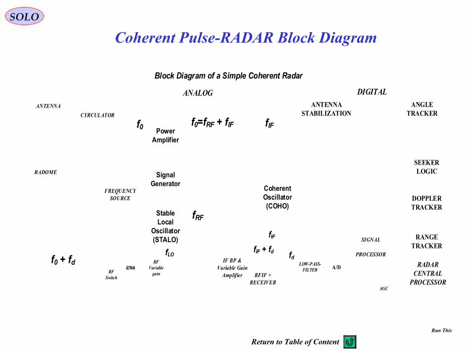
Coherent Pulse-RADAR Block Diagram
Block Diagram of a Simple Coherent Radar
f0Power
Amplifier
SignalGenerator
CoherentOscillator(COHO)
fLO
fRF
fIF
fIF
f0 + fd
fIF + fd fd
f0=fRF + fIF
IF BP &Variable Gain
Amplifier
CYRCULATOR
SIGNAL
PROCESSOR
ANGLETRACKER
DOPPLERTRACKER
RANGETRACKER
SEEKERLOGIC
RADARCENTRAL
PROCESSOR
RADOME
LOW-PASS-FILTER
ANTENNASTABILIZATION
A/D
ANALOG DIGITAL
FREQUENCYSOURCE
RFIF + RECEIVER
ANTENNA
RF Variable
gainLNA
RF Switch
AGC
Stable Local
Oscillator (STALO)
LNA
Run This
Return to Table of Content

Radar EquationRadar Cross Section Definition
SOLO
- Target Radar Cross Section (RCS) [m2]TGTσ
The incident Power Density (Irradiance) at the target is given by:
2 2 2/i i i i iS E H H E watt mµ εε µ
= × = = r r
The Power Density (Irradiance) intercepted and scatteredby the target is given by: [ ]i TGTS wattσ
The received Power Density (Irradiance) is defined as:2 2 2/r r r r rS E H H E watt m
µ εε µ
= × = = r r
Power scattered by the target in each steradian: ( ) [ ]/ 4 /i TGTS watt strσ π
Solid angle of receiver as seen from the target: [ ]2/RCVRA R strΩ=The received Power is given by: [ ]24
i TGT RCVRS A
wattR
σπ
The received Power is given also by:
2/r RCVRS A watt m
24i TGT RCVR
r RCVR
S AS A
R
σπ
=
2lim 4 rTGT R
i
SR
Sσ π
→∞=Since RCS is defined in the Far Field:

SOLO
Radar Cross Section σ of a Sphere of Radius r as a Function of the Wavelength λ
Radar Equation

SOLO Radar EquationRadar Cross Section σ of Different Bodies

Stealth aircraft are practically undetectable by sensors. They exploit the diagram to minimize scattered and reflected signals, and to focus the residuals in few directions, different from that of the sensors.
Stealth aircraft are practically undetectable by sensors. They exploit the diagram to minimize scattered and reflected signals, and to focus the residuals in few directions, different from that of the sensors.
Contributors to Target RCS
Radar Equation

SOLO
Generic Aircraft Model Scattering Center
Radar Equation

SOLO
Generic Aircraft Model Scattering Center
Radar Equation

SOLO Radar Equation

SOLO Radar Equation

SOLO Radar Equation

SOLO Radar Equation

SOLO Radar Equation
SOLO
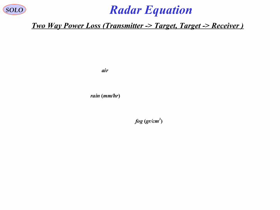
rain (mm/hr)
fog (gr/cm3)
air
Two Way Power Loss (Transmitter -> Target, Target -> Receiver )
Radar Equation

fog (gr/cm3)
rain (mm/hr)
air
Target
ECM Pod
Ground
A/C Radar
Missile, Target, Environment
fog (gr/cm3)
rain (mm/hr)
air
Target
TransmittedMainlobeEnergy
ECM Pod
Ground
A/C Radar
TransmittedSide-lobeEnergy
Missile RADAR Seeker Transmision
fog (gr/cm3)
rain (mm/hr)
air
Target
Direct-pathTarget Return
ECM Pod
Ground
A/C Radar
Target Reflected Energy Return
fog (gr/cm3)
rain (mm/hr)
air
MultipathTarget Return
Target
ECM Pod
Ground
A/C Radar
Target Multipath Return
SOLO
Target Energy Return versus Return from Unwanted Factors
• A/C Radar, Target, Environment (rain, fog, clutter)
• Radar Seeker Transmission
• Target Energy Return
• Target Multipath Return
• Target ECM Return
• Ground Clutter Return
fog (gr/cm3)
rain (mm/hr)
air Electronic Counter Measures (ECM)
Return
Target
ECM Pod
Ground
A/C Radar
Target ECM Return
fog (gr/cm3)
rain (mm/hr)
air Electronic Counter Measures (ECM)
Return
Target
Direct-pathTarget Return
ReceivedMainlobe
ClutterEnergy
ECM Pod
Ground
A/C Radar
ReceivedSide-lobeClutteerEnergy
Ground Clutter Return
fog (gr/cm3)
rain (mm/hr)
air Electronic Counter Measures (ECM)
Return
MultipathTarget Return
Target
Direct-pathTarget Return
TransmittedMainlobeEnergy
ECM Pod
Ground
A/C Radar
TransmittedSide-lobeEnergy
Target, Multipath, ECM, Clutter Returns
Run This
Radar Equation
Return to Table of Content
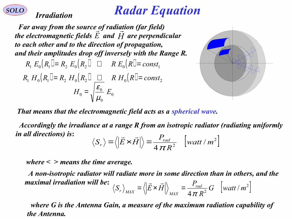
Far away from the source of radiation (far field) the electromagnetic fields and are perpendicular to each other and to the direction of propagation, and their amplitudes drop off inversely with the Range R.
Er
Hr
( ) ( ) ( ) 10202101 constRERRERRER =⇒=
( ) ( ) ( ) 20202101 constRHRRHRRHR =⇒=
That means that the electromagnetic field acts as a spherical wave.
Accordingly the irradiance at a range R from an isotropic radiator (radiating uniformly in all directions) is: [ ]2
2/
4mwatt
R
PHES rad
r π=×=
rr
00
00 EH
µε=
where < > means the time average.
A non-isotropic radiator will radiate more in some direction than in others, and the maximal irradiation will be: [ ]2
2/
4mwattG
R
PHES rad
MAXMAXr π=×=
rr
where G is the Antenna Gain, a measure of the maximum radiation capability of the Antenna.
SOLO Radar EquationIrradiation

r
MAXr
S
SG =:
Radar Equation
BϕBϑ
ϕD
ϑD
Antenna
RadiationBeam
Assume for simplicity that the Antenna radiates all the power into the solid angledefined by the product , where and are the angle from the boresight at which the power is half the maximum (-3 db).
BB ϕϑ , 2/Bϕ± 2/Bϑ±
ϑϑ
λη
ϑDB
1=ϕϕ
λη
ϕDB
1=
λ - wavelength
ϕϑ DD , - Antenna dimensions in directionsϕϑ,
ϕϑ ηη , - Antenna efficiency in directionsϕϑ,
then ( ) effBB
ADDG22
444
λπηη
λπ
ϕϑπ
ϕϑϕϑ ==⋅
=
where
ϕϑϕϑ ηη DDAeff =:
is the effective area of the Antenna.
2
4
λπ=
effA
G
SOLO

Radar Equation
Transmitter
IV
Receiver
R
1 2
Let see what is the received power on an Antenna, with an effective area A2 and range R from the transmitter, with an Antenna Gain G1
Transmitter
VI
Receiver
R
1 2
2122 4AG
R
PASP dtransmitte
rreceived π==
Let change the previous transmitter into a receiver and the receiver into a transmitter that transmits the same power as previous. The receiver has now an Antenna with an effective area A1 . The Gain of the transmitter Antenna is now G2.
According to Lorentz Reciprocity Theorem the same power will be received by the receiver; i.e.:
1224AG
R
PP dtransmittereceived π
=therefore
1221 AGAG =or
constA
G
A
G ==2
2
1
1
We already found the constant; i.e.: 2
4
λπ=
A
G
SOLO

Radar Equation
The Power Density (Irradiance) at the target is given by:
TRP
TRG
TRR
EVTarget
Transmitter
[ ]2
Pr
2/
1
4
1mW
LRL
GPS
TGTXMTRopagation
TGTTR
rTransmitte
TR
TRTRr
→
→
=π
- Transmitter Power [W]TRP
- Transmitter Antenna Gain in the Target directionTRG
- Transmitter Loss (XMTR+Antenna+Radome) ( > 1 )TRL
- Range Transmitter to Target [m2]TRR
- Propagation Loss from Transmitter to Target ( > 1 )TGTTRL →
SOLO

Radar EquationThe Power reflected by the target in the receiver direction is:
[ ]WGALRL
GPGASP
TGT
TGTTGT
TGTXMTRopagation
TGTTRTR
rTransmitte
TR
TRTRTGTTGTrTGT
σπ
→
→
==
Pr
24
1
- Target Effective area in the Transmitter direction [m2]TGTA
- Target Gain in the Receiver directionTGTG
- Propagation Loss from Target to Receiver ( > 1 )RCVRTGTL →
The Power Density [W/m2] received at the Receiver is
[ ]2
Pr
2 /1
4
1mW
LRPp
RCVRTGTopagation
RCVRTGTRCVR
TGTRCV
→
→
=π
Target
Transmitter
Receiver
SOLO
- Target Radar Cross Section (RCS) [m2]TGT TGT TGTA Gσ =

Radar Equation
[ ]2
Pr
2
Pr
2 /1
4
11
4
1mW
LRGA
LRL
GPp
RCVRTGTopagation
RCVRTGTRCVR
TGTTGT
TGTXMTRopagation
TGTTRTR
rTransmitte
TR
TRTRRCVR
TGT
→
→
→
→
=ππ
σ
- Propagation Loss at the Receiver ( > 1 )RCVRL
The Power Density [W/m2] received at the Receiver is
[ ]WL
A
LRGA
LRL
GP
LApP
ceiver
RCVR
RCVR
RCVRTGTopagation
RCVRTGTRCVR
TGTTGT
TGTXMTRopagation
TGTTRTR
rTransmitte
TR
TRTR
RCVRRCVRRCVRCVR
TGT
RePr
2
Pr
2
1
4
11
4
1
/
→
→
→
→
=
=
ππσ
The Power [W/m2] received at the Receiver is
- Effective area in the Receiver Antenna [m2]RCVRA
SOLO

Radar Equation
[ ]WL
G
LRGA
LRL
GPP
ceiver
RCVR
RCVR
RCVRTGTopagation
RCVRTGTRCVR
TGTTGT
TGTXMTRopagation
TGTTRTR
rTransmitte
TR
TRTRRCVR
TGT
Re
2
Pr
2
Pr
2 4
1
4
11
4
1
πλ
ππσ
→
→
→
→
=
the Power [W/m2] received at the Receiver is
πλ
4
2RCVR
RCVR
GA =
( ) [ ]WLLLLRR
GGPP
RCVRRCVRTGTTGTTRTRRCVRTR
TGTRCVRTRTRRCVR
→→
= 223
2
4 πσλ
Using
or
SOLO

Radar Equation
[ ]WL
G
LRGA
LRL
GPP
ceiver
RCVR
RCVRTGTopagation
TGTTRTGTTGT
TGTXMTRopagation
TGTTR
rTransmitte
TR
TRRCVR
TGT
Re
2
Pr
2
Pr
2 4
1
4
11
4
1
πλ
ππσ
→
→
→
→
=
the Power [W/m2] received at the Receiver is
( ) [ ]WLLLR
GPP
RCVRTGTTRTR
TGTTRRCVR 243
22
4 →
=π
σλor
SOLO
,RRR RCVRTR ==Collocated Transmitter & Receiver with a Common Antenna
RCVRTGTTGTTR LL →→ =GGG RCVRTR ==
Return to Table of Content


db0
db3
dbdb 326 ⋅=
dbdb 339 ⋅=db10 10
823 =
( ) dbdb 9101 −=
1
4
5
8
10 =
2
( ) dbdb 132 −=
5.24
52 =⋅( ) dbdb 134 +=
6.14/5
2 =
( ) dbdb 165 −= 2.34/5
4 =
422 =
( ) dbdb 167 += 54
54 =⋅
( ) dbdb 198 −= 4.64/5
8 =
Decibels GainDecibels = 10 log (Gain)SOLO Decibels

1010
234
111
==
=
db
db
db
db1
4
11+00.1
db5.0
4
5.01+
dbF.0
4
.01
F+
Decibels
Gain
( ) dbdb 9101 −= 4
11
4
11
8
10 +==
Decibels GainDecibels = 10 log (Gain)SOLO
db0 1
db8.0 2.1
db6.0 15.1
db4.0 10.1
dbF.0 4
.01
F+
Decibels

SOLO Decibels
Radar Parameters Often Expressed in Decibels
• Antenna Gain
• dBi (gain relative to isotropic)
• Power Loss
• dB (power out/power in)
• Power
• dBW (power related to 1 watt)
• dBm (power related to 1 milliwatt)
• Radar Cross Section (RCS)
• dBsm (RCS related to 1 square meter)
Return to Table of Content
SOLO
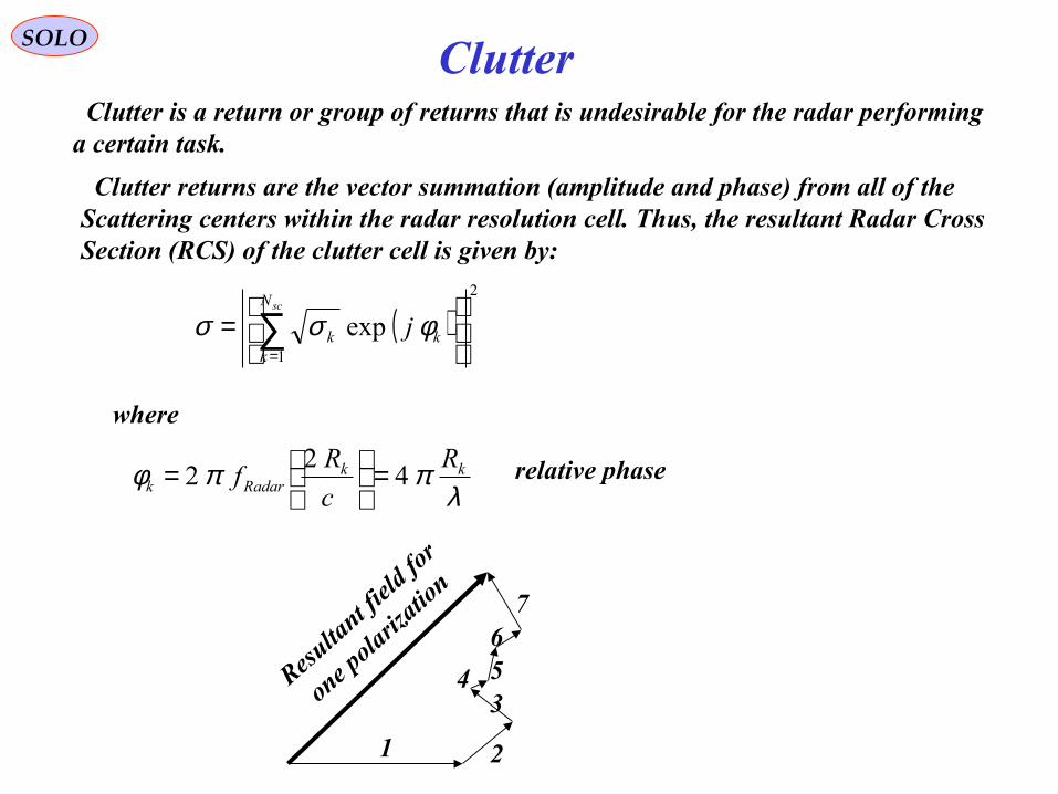
Clutter is a return or group of returns that is undesirable for the radar performinga certain task.
Clutter
Clutter returns are the vector summation (amplitude and phase) from all of theScattering centers within the radar resolution cell. Thus, the resultant Radar CrossSection (RCS) of the clutter cell is given by:
( )2
1
exp
= ∑
=
scN
kkk j φσσ
where
λππφ kk
Radark
R
c
Rf 4
22 =
= relative phase
Resulta
nt fiel
d for
one p
olariz
ation
1 2
34 5
67

SOLO
Mathematical Approaches to Characterize Clutter
Clutter
• Clutter Amplitude:
- Statistical quantities: mean, standard deviation
- Statistical distributions: probability amplitude (or power) density or cumulative probability
• Time Varying Properties:
- Correlation function, power spectral density
• Spatially Varying Properties:
- Spatial distributions, correlations, spectra

SOLO
Characterizing Clutter Using Statistical Quantities
Clutter
• Statistical quantities are useful, but knowing the amplitude distribution is equaly important
• Mean: n
x
x
n
jj∑
== 1
• Standard deviation : ( )
11
2
−
−=
∑=
n
xxn
jj
σ
Return to Table of Content

ahMV
pθ
eψ
RψcosR
Ae
Aψ
HorizontalGround
Main LobeBeam
Transmitter& Receiver
πθθπθ ≤+≤⇒−≤≤− ppp ee 0
Define a ray R from transmitter to ground, defined by the angles e,ψ, relative to Missile velocity vector.
VM is the Missile (transmitter) velocity vector, having an angleθp with the horizontal plane.
( )
≤≤−
≤+≤≥
+=
2/2/
0cossin
πψππθ
ψθ p
a
p
a e
hR
e
hR ( )
ψθ
22 cos1cos
R
he a
p −±=+
The doppler frequency shift along the ray R is given by:
( ) ( ) ( )[ ]
ψθψθ
λ
ψθθθθλ
ψλ
cossincoscos
2
cossinsincoscos2
coscos2
22
_
aap
ap
M
ppppMM
clutterd
hR
R
h
R
hV
eeV
eV
Rf
≥
+
−±=
+++==
SOLO Ground Clutter

( )
( ) ( )[ ]
+
−±=
+++=
=
R
h
R
hV
eeV
eV
Rf
ap
ap
M
ppppM
Mclutterd
θψθλ
ψθθθθλ
ψλ
sincoscos2
cossinsincoscos2
coscos2
22
_
( ) pM
aclutterd
VhRf θ
λ
ψsin
20
_
=
==
( ) ψθλ
θ
coscos20
_ pM
e
clutterd
VRf
p =+
=∞→
( ) ψθλ
πθ
coscos2
_ pM
e
clutterd
VRf
p
−=∞→=+
Altitude Line
λψ
θ
M
hR
clutterd
Vef
p
a
20,0
cos
_ =
==
=
clutterdf _
( )RangeR
( )RangeR
Clutter
No Clutter
ClutterPower
ClutterPower
Main LobeClutter(MLC)
AltitudeReturn
λMV2
pMV θ
λcos
2
AAM e
Vcoscos
2 ψλ
pMV θ
λsin
2
pMV θ
λcos
2−
( ) ApA
a
eh
ψθ cossin +
( )
( )
+=
=
ApA
aML
AAM
AAclutterd
e
hR
eV
ef
ψθ
ψλ
ψ
cossin
coscos2
,_
Main Lobe
ahMV
pθ
eψ
RψcosR
Ae
Aψ
HorizontalGround
Main LobeBeam
Transmitter& Receiver
SOLO Ground Clutter

ah
MV
e
ψ
RψcosR
HorizontalGround
Transmitter& Receiver
Main LobeBeam
Ae
Aψ
0=pθ( )
22
0
_
cos2
coscos2
−±=
=
=
R
hV
eV
Rf
aM
Mclutterd
p
ψλ
ψλ
θ
( ) 00
_
=
==ψ
aclutterd hRf
( ) ψλ
θ
cos20
_M
e
clutterd
VRf
p =+
=∞→
( ) ψλ
πθ
cos2
_M
e
clutterd
VRf
p
−=∞→=+
Altitude Line
λψ
θ
M
hR
clutterd
Vef
p
a
20,0
cos
_ =
==
=
clutterdf _
( )RangeR
( )RangeR
Clutter
No Clutter
ClutterPower
ClutterPower
Main LobeClutter(MLC)
AltitudeReturn
λMV2
0=pθ
AAM e
Vcoscos
2 ψλ
λMV2
−
AA
a
e
h
ψcossin
( )
=
=
AA
aML
AAM
AAclutterd
e
hR
eV
ef
ψ
ψλ
ψ
cossin
coscos2
,_
Main Lobe
0=pθ
SOLO Ground Clutter

Ground
ahMV
pθ
ψcosR
AeAψ
Main LobeBeam
Transmitter& Receiver
Cones ofEqui-Range
Rays
R
Projection ofTransmitter& Receiver
on the Ground
Equi-rangePoints
on the Ground
Projection on the Ground
M.L.B.
The Clutter energy froma range R are obtainedfor all points on the groundthat are at the range R fromthe Transmitter/Receiver.
Assuming a flat ground,the points on the grounda a range R > ha are locatedat the intersection of the conical surface with theapex at the Transmitter/Receiver and its altitude lineas the conic axis..
The points on the flatGround having the samerange R from theTransmitter/Receiverare circles.
SOLO Ground Clutter
Ground
ahMV
pθ
ψcosR
AeAψ
Main LobeBeam
Transmitter& Receiver
Cones ofEqui-doppler
Rays
R
Intersectionof Missile
Velocity Vectorwith the Ground
Ellipsee pθ<
Parabolee pθ=Hyperbolee pθ>
Equi-dopplerPoints
on the Ground
Projection on the Ground
M.L.B.
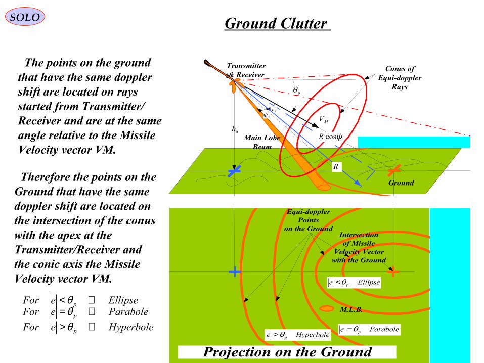
The points on the groundthat have the same dopplershift are located on raysstarted from Transmitter/Receiver and are at the same angle relative to the MissileVelocity vector VM.
Therefore the points on the Ground that have the same doppler shift are located on the intersection of the conuswith the apex at theTransmitter/Receiver and the conic axis the MissileVelocity vector VM.
EllipseeFor p ⇒<θParaboleeFor p ⇒= θHyperboleeFor p ⇒> θ
SOLO Ground Clutter

Ground
ahMV
pθ
ψcosR
AeAψ
Main LobeBeam
Transmitter& Receiver
Cones ofEqui-doppler
RaysCones ofEqui-Range
Rays
R
Projection ofTransmitter& Receiver
on the Ground
Intersectionof Missile
Velocity Vectorwith the Ground
Ellipsee pθ<
Parabolee pθ=Hyperbolee pθ>
Equi-dopplerPoints
on the Ground
Equi-rangePoints
on the Ground
Projection on the Ground
M.L.B.
SOLO Ground Clutter

SIGNALS AND CLUTTER IN A PULSE DOPPLER RADAR, IN THE LOOK-HOTIZON MODESIGNALS AND CLUTTER IN A PULSE DOPPLER RADAR, IN THE LOOK-HOTIZON MODE
SOLO Target in Ground Clutter

SIGNALS AND CLUTTER IN A PULSE DOPPLER RADAR, IN THE LOOK-HOTIZON MODE MODE, (a) A TYPICAL SITUATION: (b) MAP OF RETURNS ON THE RANGE/VELOCITY PLANE: (c) FOLDING OFCLUTTER OVER THE RANGE AXIS (LOW PRE): (d) CONCENTRATION OFRETURNS ON THE VELOCITY AXIS (HIGH PRF).
SIGNALS AND CLUTTER IN A PULSE DOPPLER RADAR, IN THE LOOK-HOTIZON MODE MODE, (a) A TYPICAL SITUATION: (b) MAP OF RETURNS ON THE RANGE/VELOCITY PLANE: (c) FOLDING OFCLUTTER OVER THE RANGE AXIS (LOW PRE): (d) CONCENTRATION OFRETURNS ON THE VELOCITY AXIS (HIGH PRF).
SOLO Target in Ground Clutter

SOLOGround Clutter
Illuminated Ground Area Resolution Cell : Beam Limitted Case
The Main Beam Clutter (Ground) Area in Range Resolution Cell when
is give (see Figure) by:
( ) ( ) pazcRA θϕτ cos/2/tan2/2Clutter =
Ground
Main LobeBeam
Transmitter& Receiver
( ) ( )2//2/tan2tan τϕθ cR elp <
R – range to ground along beam center
φaz – angular beam width in azimuth
φel – angular beam width in elevation
θp –beam grazing angle
τ – pulse width [sec]c – speed of light 3 108 m/sec
( )Clutter Clutter pAσ σ θ=
σ – ground reflectivity as function of grazing angle

SOLOGround Clutter

SOLOGround Clutter
Return to Table of Content

SOLOClutter
Illuminated Volume Resolution Cell (Pulse Limitted) The Volume Clutter in Range Resolution Cell is give (see Figure) by:
( )2/4
2Clutter τϕϕπ
cRV elaz=
R – range to ground along beam center
φaz – angular beam width in azimuth
φel – angular beam width in elevation
τ – pulse width [sec]c – speed of light 3 108 m/sec
Main LobeBeam
Transmitter& Receiver
Choose scatters on the main beam center Groundkk RRuntilkRkR ≥=∆= ,2,1
RADAR
Ik f
cwhere
sVf =⋅= λ
λ12
r
Their Doppler is given by
According to Range and Doppler of each scatter determine the Range-Doppler cell (i,j) for the scatter.

Clutter returns are the vector summation (amplitude and phase) from all of the scattering centers within the radar resolution cell.
SOLO Clutter
The Clutter is obtained by integration (summation) of the signals from the same range-doppler cells:
where
Nsc – number of scatters in the volume VClutter
σk– Radar Cross Section of scatter kRk– Range to scatter k
The equivalent Radar Cross Section σClutter of the clutter in the resolution cell of volume VClutter is:
( )2/4
2Clutter τϕϕπ
cRV elaz=
g (0,0) ≈ 1 – antenna patternR – Range to the center of the volume VClutter
See Tildocs # 763310 v1
( ) ( )( )
∑=
+−=Σ
jiN
k
kkk
trver
RcvrXmtr
sc
c
c
RRR
jL
GGPji
,
12
k
kscatter
3
20
2
ClutterVolume 2
22exp
R4,
πσ
πλ
Illuminated Volume Resolution Cell (Pulse Limitted)
∑=
==scN
k k
kscatterClutterClutter
RRV
14
4 σησ ∑
=
=scN
k k
kscatter
Clutter RV
R
14
4 ση
Since the Volume Clutter is on the Main-Beam the effect of it on angle errors is like that of the radar noise.
Return to Table of Content
Main LobeBeam
Transmitter& Receiver

MultipathTarget Return
Target
Ground
A/C RADAR
Target Multipath Return
SOLO
Multipath Return
Target Multipath is the Received Signalfor the mirror reflection the target relativeto Earth surface.
The vector position of the Target relative to earth is
LTLTLTT zhyYxXR 111 ++=r
The vector position of the mirrored Target relative to earth is
( ) LLTTLTLTLTMT zzRRzhyYxXR 112111_ ⋅−=−+=rrr
The vector of the signal received by Seeker from the i Target scatter is
IT RRRrrr
−=
The vector of the signal received by Seeker from the mirrored Target is
( ) ( ) LLTLLTITM zzRRzzRRRR 112112 ⋅−=⋅−−=rrrrrr
Clutter
hT – altitude above ground surface

SOLO
Multipath Return – Range Discrimination
The Target Range to Seeker is
( )22ITIT hhXR −+= −
Let compute
Clutter
The Range of the Mirror Target to Seeker is
( ) RhhXR ITITM ≥++= −22
( ) ( ) ( ) ( ) ITITITMMM hhhhhhRRRRRR 42222 =−−+=−=+−
R
hh
RR
hhRR IT
RRR
M
ITM
M 24 2≈+
≈+
=−
..2
GRR
hhRR IT
M ≤≈−If , for all Target scatters k, we cannot distinguish between Target and Target’s Mirror
..2
GRR
hhRR IT
M >≈−If , for some Target scatters, we can distinguish between Target and Target’s Mirror and we willchoose the echoes with the smallest range
MultipathTarget Return
Target
Ground
A/C RADAR
Target Multipath Return

SOLO
Multipath Return – Doppler Discrimination
The Target Range-Rate to Seeker is
( )22ITIT
IITTITIT
hhX
hhhhXXR
−+
++=
−
−−
Let compute
Clutter
The Range-Rate of the Mirror of Target to Seeker is
( ) ( ) ( )( )
( )( )
( )( )[ ] ( )[ ] Mi
MiIT
ITITITIT
IITTITITIT
ITIT
IITTITIT
ITIT
IIiTTITITMMM
RR
RRhh
hhXhhX
hhhhXXhh
HHX
HHHHXX
HHX
HHHHXXRRRRRR
44
2222
2
22
2
22
2
22
=++−+
++=
=++
++−
−+++
=−=+−
−−
−−
−
−−
−
−−
024
3
2
>≈+
=−≈+
MIT
RRR
M
M
M
ITMi RR
R
hh
RR
RR
RR
hhRR
M
..2
3GDRR
R
hhRR M
ITM ≤≈− If we cannot distinguish between
Target and Target’s Mirror
..2
3GDRR
R
hhRR M
ITM >≈−
If we can distinguish between Target and Target’s Mirror and we don’t have a Multipath problem.
( )22ITIT
IITTITITM
hhX
hhhhXXR
++
++=
−
−−
Assume that Target & Mirror Target are in the same Range Gate.
MultipathTarget Return
Target
Ground
A/C RADAR
Target Multipath Return

SOLO
Multipath Return – Angular Discrimination
We found:
( ) ( ) LLTLLTITM zzRRzzRRRR 112112 ⋅−=⋅−−=rrrrrr
Clutter
The angular separation between Target Scatter k and Target Mirror Scatter k is:
( )RR
RzzR
RR
RR
M
LLT
M
M
rrrr×⋅
−=× 11
2
Multipath Return – Range – Doppler Map According to Range and Doppler of each scatter mirror:
determine the Range-Doppler cell (i,j) for the scatter mirror.
( ) kITkITMk RhhXR ≥++= −22 ( )
( )22ITkITk
IITkTkITkITkMk
HHX
hhhhXXR
++
++=
−
−−
integer=+= mRRmR kambiguoussunambiguouMk
RADAR
MkMk f
cwhere
Rf == λ
λ2
integer=+= nffnf kambiguoussunambiguouMk
( )RRIntegi kambiguousk ∆= /
( )ffIntegj kambiguousk ∆= /
MultipathTarget Return
Target
Ground
A/C RADAR
Target Multipath Return

SOLO
Multipath Return – Signal Power
Assume that The Target and it’s Mirror can be represented each by Nsc scatters ( k=1,Nsc)
Clutter
The Mirror signal received by the Seeker from scatter k passes three paths:
TGTXMTRopagation
TGTTRk
rTransmitte
TR
trXmtr
LRL
GP
→
→
Pr
2
1
4
1
π1. Transmitted power from Seeker to Target Scatter k at the distance Rk:
2. Reflected by the target scatter k and reaching the ground at the distance ( ) ( )[ ] 2/122_1 TkIIT
TkI
Tkk hhX
hh
hR ++
+=
GNDTGTopagation
GNDTGTk
TGTTGT LRGA
TGT
→
→
Pr
21
1
4
1
πσ
3. Reflected by the ground and reaching the Seeker at the distance ( ) ( )[ ] 2/122_2 TkIIT
TkI
Ik hhX
hh
hR ++
+=
ReceivernPropagatio
22
1
4
1
RCVR
RCVR
GNDTGT
RCVRGNDk
GND L
A
LR
→
→πσ
πλ
4
2RCVR
RCVR
GA =
MultipathTarget Return
Target
Ground
A/C RADAR
Target Multipath Return

SOLO
Multipath Return – Signal Power
Therefore the received power from the k scatter mirror is:
Receiver
2
nPropagatio
22
Pr
21
Pr
2
1
4
1
4
11
4
11
4
1
RCVR
RCVRant
GNDTGT
RCVRGNDk
GND
GNDTGTopagation
GNDTGTk
kScatterkScatter
TGTXMTRopagation
TGTTRk
rTransmitte
TR
antXmtrM L
GG
LRLRGA
LRL
GPP
kScatter
k πλ
πσ
ππσ
→
→
→
→
→
→
=
Clutter
( ) ( )[ ] 2/122_1 TkIIT
TkI
Tkk hhX
hh
hR ++
+= ( ) ( )[ ] 2/122
_2 TkIITTkI
Ik hhX
hh
hR ++
+=
( ) ( )( )( ) ( )
+++++++−=Σ ∑
=
Σ
ccj
gG
L
GGPji
jiN
k
ClutterkElkAzproc
trver
RcvrXmtr
k2k1kk2k1kk2k1k,
1 k2k1k
kscatter
proc
Targ
3
20
2
TargetMultipath
RRRRRRRRR
2expRRR
,
L4,
πσσεε
πλ
( )( )
22
21
2
2Targ
3
20
2 ,
4 kkk
ClutterkScatterkElkAz
proc
proc
trver
RcvrXmtrM
RRR
g
L
G
L
GGPP
k
σσεεπ
λ Σ=or:
where: ( )kElkAzant gGG εε ,0 Σ=RCVRRCVRGNDGNDTGTTGTTRTRtrver LLLLLL →→→=
proc
procRcvrRCVR L
GGG
Targ
=
The Target Multipath received signal is obtained by integration (summation) of the signals from the same range-doppler cell (i,j):
in the same way:
( ) ( )( )( ) ( )
+++++++−=∆ ∑
=
∆
ccj
gG
L
GGPji
jiN
k
ClutterkElkAzElAzproc
trver
RcvrXmtr
k2k1kk2k1kk2k1k,
1 k2k1k
kscatter,
proc
Targ
3
20
2
Az/ElTargetMultipath
RRRRRRRRR
2expRRR
,
L4,
πσσεε
πλ
Return to Table of Content

SOLOElectronic Counter Measures (ECM)
SOLOElectronic Counter Measures (ECM)

SOLOElectronic Counter Measures (ECM)

SOLOElectronic Counter Measures (ECM)

SOLOElectronic Counter Measures (ECM)

SOLOElectronic Counter Measures (ECM)

SOLOElectronic Counter Measures (ECM)

SOLOElectronic Counter Measures (ECM)

SOLOElectronic Counter Measures (ECM)

SOLOElectronic Counter Measures (ECM)
SOLOElectronic Counter Measures (ECM)

SOLOElectronic Counter Measures (ECM)

SOLOElectronic Counter Measures (ECM)

SOLOElectronic Counter Measures (ECM)

SOLOElectronic Counter Measures (ECM)
Return to Table of Content

SOLO Signal Processing
Return to Table of Content

SOLO Signal Processing
Collecting Pulsed Radar Data: 1 Pulse, Multiple Range-Gates Samples
• when using a coherent receiver, each range sample comprises one “I” sample and one “Q” sample, forming one complex number I+j Q.• Each range cells contains an echo from a different range interval.
• Also called Range-Bins, Range-Gates, Fast-Time Samples.

SOLO Signal Processing
Collecting Pulsed Radar Data: Multiple Pulses
• when using a coherent receiver, each range sample comprises one “I” sample and one “Q” sample, forming one complex number I+j Q.• Repeat for multiple pulses in a “coherent processing interval” (CPI) or “dwell”
Sequence of samples for a fixed range bin represents echoes from same range interval over a period of time.

SOLO Signal Processing
Perform FFT in Each Range Gate
After FFT a Range-DopplerMap is obtained for SignalProcessing
FFT
Run This

SOLO Signal Processing
Perform FFT in Each Range Gate
Data-cube for Signal Processing
Repeat the Operation for each Receiver Channel (Σ,ΔAz,ΔEl,Γ for monopulse antenna or Σi,j for each element in an Electronic Scanned Antenna)
Range – Doppler Cells in Σ and ΔAz, ΔEl
FFT
FFT
FFT
FFT
Run This

SOLO Signal Processing
Adaptive algorithms use additional data from the cube for weight estimation.
Datacube for Signal Processing
Standard radar signal processing algorithms correspond to operating in 1- or 2-D alongvarious axes of the data-cube
Space-Time Adaptive Processing:2-D joint adaptive weighting acrossantenna element and pulse number
Beamforming:1-D weighting acrossElectrical Scan Antennaelement number
Pulse Compression:1-D convolution alongthe range axis(“fast time”)
Synthetic Aperture Imaging:2-D matched filtering in slowand fast time
Doppler Processing:1-D filtering or spectralanalysis along the pulse axis(“slow time”)
Run This

SOLO Signal Processing
Range – Doppler Cells in Σ and ΔAz, ΔEl

SOLOWindowing
• Windowing is used for DFT data to reduce Doppler side lobes
• Windowing widen main lobe and this decreases Doppler resolution
• Windowing reduces the peak of the DFT producing a processing loss, PL
• Windowing causes a modest signal to noise (S/N) loss, called loss in peak gain, or LPG.
Windows are an overlay applied to a given time series to improve the spectral qualityof the data base.
Signal Processing

SOLOWindowing
Rectangular [ ] ≤≤
=otherwise
Mnnw
,0
0,1
Bartlett(triangular) [ ]
≤<−≤≤
=otherwise
MnMMn
MnMn
nw
,0
2/,/22
2/0,/2
Hanning
Hammming
[ ] ( ) ≤≤−
=otherwise
MnMnnw
,0
0,/2cos5.05.0 π
[ ] ( ) ≤≤−
=otherwise
MnMnnw
,0
0,/2cos46.054.0 π
Blackman [ ] ( ) ( ) ≤≤+−
=otherwise
MnMnMnnw
,0
0,/4sin08.0/2cos5.042.0 ππ
Julius Ferdinand von Hann (1839 -1921)
Richard Wesley Hamming (1915 –1998)
Signal Processing
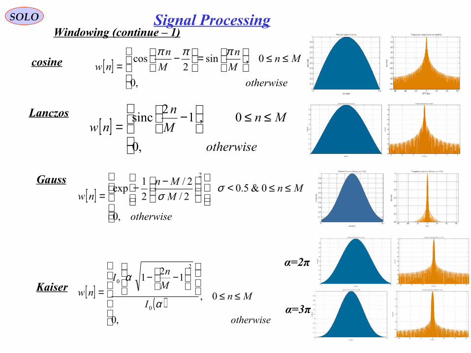
SOLOWindowing (continue – 1)
cosine
[ ]
≤≤<
−−=
otherwise
MnM
Mnnw
,0
0&5.02/
2/
2
1exp
2
σσ
Lanczos[ ]
≤≤
−
=otherwise
MnM
nnw
,0
0,12
sinc
Gauss
[ ]
≤≤
=
−
=otherwise
MnM
n
M
nnw
,0
0,sin2
cosπππ
[ ]( )
≤≤
−−
=
otherwise
MnI
Mn
I
nw
,0
0,
12
1
0
2
0
α
αKaiser
α=2π
α=3π
Signal Processing

SOLOWindowing (continue – 2)
Bartlett–Hann window
( )
38.0;42,0;62.0
1
2cos
2
1
1
210
210
===
−−−
−−=
aaa
N
na
N
naanw
π
Bartlett–Hann window; B=1.46 Low-resolution (high-dynamic-range) windows
Nuttall window, continuous first derivative
( )
012604.0;144232.0;487396,0;355768.0
1
6cos
1
4cos
1
2cos
3210
3210
====
−−
−+
−−=
aaaa
N
na
N
na
N
naanw
πππ
Nuttall window, continuous first derivative; B=2.02
Blackman–Harris window
( )
01168.0;14128.0;48829,0;35875.0
1
6cos
1
4cos
1
2cos
3210
3210
====
−−
−+
−−=
aaaa
N
na
N
na
N
naanw
πππ
Blackman–Nuttall window Blackman–Harris window, B=1.98
Blackman–Nuttall window, B=3.77
( )
0106411.0;1365995.0;4891775,0;3635819.0
1
6cos
1
4cos
1
2cos
3210
3210
====
−−
−+
−−=
aaaa
N
na
N
na
N
naanw
πππ
Signal Processing

SOLOWindowing (continue – 3)
Dolph-Chebyshev window
( ) ( )[ ]
( ) ( )[ ]( ) ( )4,3,2,10cosh
1cosh
1,,2,1,0,coshcosh
coscoscos
1
1
1
≈
=
−=
=
=
−
−
−
αβ
β
πβω
ω
α
N
NkN
Nk
N
W
WIDFTnw
k
k
The α parameter controls the side-lobe level via the formula:
Side-Lobe Level in dB = - 20 α
The Dolph-Chebyshev Window (or Dolph window) minimizes the Chebyshev norm of the side lobes for a given main lobe width 2 ωc:
( ) ( ) ωωω WWsidelobescwwww >=∞= ∑=∑ maxmin:min
1,1,
The Chebyshev norm is also called the L - infinity norm, uniform norm, minimax norm, or simply the maximum absolute value.
Signal Processing

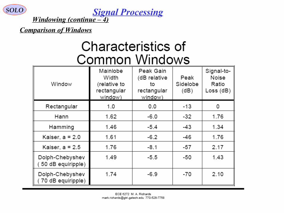
SOLOWindowing (continue – 3)
Comparison of Windows
Signal Processing

SOLO
Windowing (continue – 3)
Comparison of Windows
WindowType
Peak Sidelobe
Amplitude (Relative)
Approximate Width of Mainlobe
Peak Approximation
Error20 log10δ
(dB)
Equivalent Kaiser
Windowβ
Transition Width
of EquivalentKaiser
Window
Rectangular -13 4π/(M+1) -21 0 1.81π/M
Bartlett -25 8π/M -25 1.33 2.37π/M
Hanning -31 8π/M -44 3.86 5.01π/M
Hamming -41 8π/M -53 4.86 6.27π/M
Blackman -57 12π/M -74 7.04 9.19π/M
Signal Processing
SOLOWindowing (continue – 4)
Comparison of Windows
Signal Processing

SOLOWindowing (continue – 5)
Effect of Window in the Fourier Transform
• Good Effects
- Reduction of sidelobes
- Reduction of straddle loss
• Bad Effects
- Reduction in peak
- Widening of mainlobe
- Reduction in SNR
No Window
Hamming Window
∑−
=
1
0
21 N
nnwN
21
0
1
0
2
1
∑
∑−
=
−
=
N
nn
N
nn
w
w
N
Signal Processing
Run This

Signal Processing

Signal Processing

Signal Processing

Signal Processing

Signal Processing

Signal Processing

SOLO Signal Processing
Generation of Σ , ΔAz, ΔEl Range – Doppler Maps
The Parameters defining the Range – Doppler Maps are:
Δ R – Map Range Resolution
Δ f – Map Doppler Resolution
RUnambiguous – Unambiguous Range
fUnambiguous – Unambiguous Doppler
Range – DopplerCell
Range – DopplerMap
f
fM
R
RN sunambiguousunambiguou
∆=
∆= &
Range Gates are therefore i = 1, 2, …, NNumber of Range-Doppler Cells = N x M
Doppler Gates are therefore j = 1, 2, …, M
Note: The Map Range & Doppler resolution (Δ R, Δ f) may change as function of Radar task (Search, Detection, Acquisition, Track). This is done by choosingthe Pulse Repetition Interval (PRI) and the number of pulses in a batch.
resolutionresolution ffRR ≥∆≥∆ &

SOLO Signal Processing Generation of Σ , ΔAz, ΔEl Range – Doppler Maps (continue – 1)
The received signal from the scatter k is:
( ) ( )[ ] ( ) ( )ttTktttTkttfCts ddkdkrk
rk ++≤≤++−= τθπ2cos
Ckr – amplitude of received signal
td (t) – round trip delay time given by ( )2/c
tRRtt kk
d
+=
θk – relative phase
The received signal is down-converted to base-band in order to extract the quadrature components. More precisely sk
r (t) is mixed with: ( ) [ ] τθπ +≤≤+= TktTktfCty kkk 2cos
After Low-Pass filtering the quadrature components of Σk, ΔAz k or ΔEl k signals are:
( ) ( )( ) ( )
==
tAtx
tAtx
kkQk
kkIk
ψψ
sin
cos
( ) ( )
+−≅−=
c
tR
c
Rfttft kkkdkk
2222 ππψ
The quadrature samples are given by:( ) ( )
+−≅=
c
tR
c
RfjAjAtX kkkkkkk
222expexp πψ
Ak - amplitude of Σk, ΔAz k or ΔEl k signals ψk - phase of Σk, ΔAz k or ΔEl k signals
( )
+−
+≅+=
c
tR
c
RfAj
c
tR
c
RfAxjxtX kk
kkkk
kkQkIkk
222sin
222cos ππ

SOLO Signal Processing Generation of Σ , ΔAz, ΔEl Range – Doppler Maps (continue – 2)
The received signal from the scatter k is:
The energy of the received signal is given by: ( ) ( ) 2kkkk AtXtXP == ∗
( )
+−
+≅+=
c
tR
c
RfAj
c
tR
c
RfAxjxtX kk
kkkk
kkQkIkk
222sin
222cos ππ
where * is the complex conjugate.
Therefore:kk PA =
Return to Table of Content

Decision/Detection TheorySOLO
Hypotheses
H0 – target is not present
H1 – target is present
Binary Detection
( )0Hp - probability that target is not present
( )1Hp - probability that target is present
( )zHp |0 - probability that target is not present and not declared (correct decision)
( )zHp |1 - probability that target is present and declared (correct decision)
Using Bayes’ rule: ( ) ( ) ( )∫=Z
dzzpzHpHp |00( ) ( ) ( )∫=
Z
dzzpzHpHp |11
( )zp - probability of the event Zz ⊂
Since p (z) > 0 the Decision rules are:
( ) ( )zHpzHp || 01 < - target is not declared (H0)
( ) ( )zHpzHp || 01 > - target is declared (H1) ( ) ( )zHpzHpH
H
|| 01
0
1
<>

Decision/Detection TheorySOLO
Hypotheses H0 – target is not present H1 – target is present
Binary Detection
( )zHp |0 - probability that target is not present and not declared (correct decision)
( )zHp |1 - probability that target is present and declared (correct decision)
( )zp - probability of the event Zz ⊂
Decision rules are: ( ) ( )zHpzHpH
H
|| 01
0
1
<>
Using again Bayes’ rule:
( ) ( ) ( )( ) ( ) ( ) ( )
( )zp
HpHzpzHp
zp
HpHzpzHp
H
H
00
011
1
||
||
0
1
=<>=
( )0| Hzp - a priori probability that target is not present (H0)
( )1| Hzp - a priori probability that target is present (H1)
Since all probabilities arenon-negative
( )( )
( )( )1
0
0
1
0
1
|
|
Hp
Hp
Hzp
Hzp
H
H
<>

Decision/Detection TheorySOLO
Hypotheses
( )1| Hzp - a priori probability density that target is present (likelihood of H1)
( )0| Hzp - a priori probability density that target is absent (likelihood of H0)
Detection Probabilities
( ) M
z
D PdzHzpPT
−== ∫∞
1| 1
( )∫∞
=Tz
FA dzHzpP 0|
( ) D
z
M PdzHzpPT
−== ∫∞−
1| 1
PD - probability of detection = probability that the target is present and declared
PFA - probability of false alarm = probability that the target is absent but declared
PM - probability of miss = probability that the target is present but not declared
T - detection threshold
DP
FAP
( )1| Hzp( )0| Hzp
MPz
Tz
( )( ) T
Hzp
Hzp
T
T =0
1
|
|
H0 – target is not present H1 – target is present
Binary Detection
( )( )
( )( ) THp
Hp
Hzp
HzpLR
H
H
=<>=
1
0
0
1
0
1
|
|:Likelihood Ratio Test (LTR)

Decision/Detection TheorySOLO
Hypotheses
Decision Criteria on Definition of the Threshold T
1. Bayes Criterion
DP
FAP
( )1| Hzp( )0| Hzp
MPz
Tz
( )( ) T
Hzp
Hzp
T
T =0
1
|
|
H0 – target is not present H1 – target is present
Binary Detection
( )( )
( )( ) THp
Hp
Hzp
HzpLR
H
H
=<>=
1
0
0
1
0
1
|
|:Likelihood Ratio Test (LTR)
The optimal choice that optimizes the Likelihood Ratio is ( )( )1
0
Hp
HpTBayes =
This choose assume knowledge of p (H0) and P (H1), that in general are not known a priori.
2. Maximum Likelihood Criterion
Since p (H0) and P (H1) are not known a priori, we choose TML = 1
( )1| Hzp( )0| Hzp
MP z
Tz
( )( ) 1
|
|
0
1 == ML
T
T THzp
Hzp
DP
FAP

Decision/Detection TheorySOLO
Hypotheses
Decision Criteria on Definition of the Threshold T (continue)
3. Neyman-Pearson Criterion
DP
γ=FAP
( )1| Hzp( )0| Hzp
MPz
Tz
( )( ) PN
T
T THzp
Hzp−=
0
1
|
|
H0 – target is not present H1 – target is present
Binary Detection
( )( )
( )( ) THp
Hp
Hzp
HzpLR
H
H
=<>=
1
0
0
1
0
1
|
|:Likelihood Ratio Test (LTR)
Neyman and Pearson choose to optimizes the probability of detection PD
keeping the probability of false alarm PFA constant.
Egon Sharpe Pearson1895 - 1980
Jerzy Neyman1894 - 1981
( )∫∞
=T
TT
zzDz
dzHzpP 1|maxmax ( ) γ== ∫∞
Tz
FA dzHzpP 0|constrained to
Let use the Lagrange’s multiplier λ to add the constraint
( ) ( )
−+= ∫∫
∞∞
TT
TT
zzzz
dzHzpdzHzpG 01 ||maxmax γλ
Maximum is obtained for:
( ) ( ) 0|| 01 =+−=∂∂
HzpHzpz
GTT
T
λ( )( ) PN
T
T THzp
Hzp−==
0
1
|
|λ
zT is define by requiring that: ( ) γ== ∫∞
Tz
FA dzHzpP 0|

Decision/Detection TheorySOLO
Return to Table of Content

SOLO SEARCH & DETECT MODE During Search Mode the RADAR Seeker performs the following tasks:
• Slaves the Seeker Gimbals to the Designation Target direction (like in Slave Mode).
• Transmits the RF (by choosing the best waveform).
• Receives the returning RF.
• Compute the Σ Range-Doppler Map, chooses the Detection Threshold and policy.
• Perform Detections Clustering and compute Range and Doppler spread.
Note: Here is important to define the number of Batches that are needed to obtain the predefined probability of detection, the False Alarm Rate (FAR) and to resolve the differentdetections, i.e. the time necessary to perform this task.
• If a Detection is in the Target Designation (Uncertainty) Window we go to Acquisition Mode.

Target returns are the summation of signals (amplitude and phase) from all of the scattering centers within the radar resolution cell.
SOLO Target RCS
where
Nsc – number of scatters in the volume VResol
σk– Radar Cross Section of scatter k
Rk– Range to scatter k
The equivalent Radar Cross Section σTarget of the target in the resolution cell of volume VResol is:
2Nscatter i4
Target Resol 4i 1 iR
gV R
σσ η Σ
=
= = ∑24 N
scatter i
4i 1Resol iR
gR
V
ση Σ
=
= ∑ ( )2/4
2Resol τϕϕπ
cRV elaz=
gΣ (εAz,εEl) – antenna sum pattern ( gΣ(0,0)=1 )
R – Range to the center of the volume VResol
( ) ( )( )( )
∑=
Σ
+−=Σ
jiN
k
kkk
kElkAzproc
trver
RcvrXmtr
sc
ccR
RRj
gG
L
GGPji
,
12
k
kscatter
proc
Targ
3
20
2
Targ 22
2expR
,
L4,
πσεε
πλ
In the same way:
gΔ (εAz,εEl) – antenna difference pattern ( gΔ(0,0)=0 )
R G A AN TG EE S
DOPPLERFILTERS
Range-Doppler S cells
Detections
According to Range and Doppler of each scatter determine theRange-Doppler cell (i,j) for the scatter.
( ) ( )( )( )
∑=
∆
+−=∆
jiN
k
kkk
kElkAzElAzproc
trver
RcvrXmtr
sc
ccR
RRj
gG
L
GGPji
,
12
k
kscatter,
proc
Targ
3
20
2
Az/ElTarg 22
2expR
,
L4,
πσεε
πλ

SOLO SEARCH & DETECT MODE
According to the position of Target Uncertainty Window (TUW) versus Clutter chose the Range – Doppler magnitude (Runambiguous and funambiguous) by defining the Pulse Repetition Frequency (PRF) and the number of pulses in the batch, and choose resolution Δ R and Δ f.
Improvements
1. Change Range-Doppler cells indexes i,j tobring the Target Uncertainty Window inthe middle of the Range-Doppler Map
2. Choose on the Range-Doppler Map aarea that includes the Target UncertaintyWindow and perform Ground Cluttercomputations only for this area (we may addGround Clutter computations in Main Lobeand Altitude Line: Rk = hI).
Transmits the RF (by choosing the best waveform).
Computation of the Σ Range-Doppler Map, chooses the Detection Threshold and policy

SOLO SEARCH & DETECT MODE
Computation of the Σ Range-Doppler Map, chooses the Detection Threshold and policy (continue – 1)
• Computation of Noise Threshold in each cell: ( ) ( ) ( ) BFTkjijijiN NoiseNoise 0,,, =Σ⋅Σ= ∗
• Computation of Clutter Power in CFAR Window cells (Cells in area around Target Uncertainty Window):
( ) ( ) ( ) ∗Σ⋅Σ= jijijiCCFAR
,,,
• Computation of Signal Power in Target Uncertainty Window cells:
( ) ( ) ( )∗Σ⋅Σ= jijijiS ,,,Window
yUncertaintTarget
• For each Range-Doppler Cell (i,j) perform the summation of complex signals for all the scatters in this cell:
∑∑∑===
∆=∆∆=∆Σ=Σjijiji N
kkEljiEl
N
kkAzjiAz
N
kkji
,,,
1,
1,
1, ,,

SOLO SEARCH & DETECT MODEComputation of the Σ Range-Doppler Map, chooses the Detection Threshold and policy (continue – 2).
DOPPLERWINDOW
R W A IN NG DE O W
R G A AN TG EE S
DOPPLERFILTERS
S cells
CFARWindow
R∆
f∆
Target Uncertainty
Window
( ) ( ) ( )[ ]∑ ∗+ Σ⋅Σ=
n
j WindowCFARNoiseClutter jiji
niC ,,
1
Guard(Gap)
Window
• Computation of Clutter + Noise Threshold
• Coherent Detection:
( ) ( )( ) ( ) ClutterThjiNiCIf
ClutternoThjiNiCIf
NoiseClutter
NoiseClutter
⇒+>⇒+≤
+
+
1,
1,
( ) NoiseThNjiS +≥Window
yUncertaintTarget,
( ) ( ) ( )[ ]∑ ∗+ Σ⋅Σ=
n
j WindowCFARNoiseClutter jiji
niC ,,
1
1. If no Clutter declare a Detection in the (i,j) cell of the Target Window if
ThNoise is chosen to assure a predefinedProbability of Detection pd and of False Alarm pFA
( ) NoiseClutterNoiseClutter ThCjiS ++ +≥Window
yUncertaintTarget,
2. If Clutter declare a Detection in the (i,j) cell of the Target Window if
ThNoise is chosen to assure a predefinedProbability of Detection pd and of False Alarm pFA

SOLO SEARCH & DETECT MODEComputation of the Σ Range-Doppler Map, chooses the Detection Threshold and policy (continue – 3).
• Coherent Detection (M-out-of-N):How to Increase Probability of Detection and Reduce Probability of False Alarm:
Suppose that by Coherent Detection using one Range – Doppler Map we haveProbability of Detection pd and Probability of False Alarm pfa.To Increase Probability of Detection to pD and Reduce Probability of False Alarmto pFA we use N consecutive batches (at different PRFs) , in each of them performing the Coherent Detection procedure. We declare a detection in the if we have at least M Detections for corresponding resolved Range-Doppler cells. In this way:
( ) ( )∑=
−−−
=N
Ml
lNd
ldD pp
lNl
NP 1
!!
!
( ) ( )∑=
−−−
=N
Ml
lNfa
lfaFA pp
lNl
NP 1
!!
!
Example: pd = 0.6, pfa = 10-3, N = 4, M = 2 gives pD = 0.82, pFA = 6 x10⁻⁶
Since we use different PRFs,to obtain correlation betweenDetections we must resolve theRange-Doppler ambiguities.

SOLO SEARCH & DETECT MODEComputation of the Σ Range-Doppler Map, chooses the Detection Threshold and policy (continue – 4).
How to Increase Probability of Detection and Reduce Probability of False Alarm:
• Non-Coherent Detection:
To Increase Probability of Detection we use N consecutive batches, we compute thepower of each (i,j) cell, , in each Range-Doppler Map and we add (non-coherently) the powers of each corresponding (i,j) cell to obtaina non-coherent Range-Doppler Map. Now we perform the detection procedureas described before to declare a Detection.
( ) ( ) ( )∗Σ⋅Σ= jijijiS ,,,

SOLO SEARCH & DETECT MODEPerform Detections Clustering and compute Range and Doppler spread.
• Clustering
The Target signal may be spread in more then one Σ Range-Doppler cell. Clustering Process is to group the detections in the Σ Range-Doppler Map.
Group l parameters are mean and spread:
( )( )
( )( )∑
∑∑
∑==
il
ill
l
il
ill
l jiS
jiSii
jiS
jiSii
,
,&
,
, 2
2
( )( )
( )( )∑
∑∑
∑==
il
ill
l
il
ill
l jiS
jiSjj
jiS
jiSjj
,
,&
,
, 2
2
Range
Doppler
integer=∆+= mRiRmRlsunambiguoul
RiillRl
∆−= 22σ
integer=∆+= nfifnflsunambiguoul
fjjllf l
∆−= 22σ
If the spread of Target Range/Doppler spread σRl/ σRl are too high, we may remove theTarget detection assumption and declare the group l as Clutter.
lRadar
lf
f
cR
2=
ll fRadar
R f
c σσ2
=

SOLO SEARCH & DETECT MODEPerform Detections Clustering and compute Range and Doppler spread.
• Altitude Line and Main Lobe Clutter
The Interceptor altitude above ground hI is unknown. Therefore is necessary to search for Altitude Line and the Main Lobe Clutter in order to properly choosethe PRFs and the Σ Range-Doppler Map.
clutterdf _
( )RangeR
( )RangeR
Clutter
No Clutter
ClutterPower
ClutterPower
Main LobeClutter(MLC)
Altitude Return
λMV2
pMV θ
λcos
2
AAM eV
coscos2 ψ
λ
pMV θ
λsin
2
pMV θ
λcos
2−
TargetRange
TargetDoppler
( ) ApA
I
e
h
ψθ cossin +
12
N1 2 M
Range-Doppler Map
• Check that the detection are from returns in the Main Lobe by comparing the signal power with the antenna Γuard power.
( ) ( ) ( ) ∗∗ Γ⋅Γ>Σ⋅Σ= jijijiS ,,,Window
yUncertaintTarget
If true the received signal is in the Main Lobe If not the received signal is in the Side Lobe and therefore rejected.

SOLO ACQUISITION MODE
During Acquisition Mode the RADAR Seeker performs the following tasks:
• Slaves the Seeker Gimbals to the Designated Target direction.• The Angular Tracker is initialized.
• Confirms that the Detection is steady and in the Designated Zone by solving the ambiguities in Range and Doppler by using a number of Batches with different PRFs (Pulse Repetition Frequency).
• The Angular Tracker uses the Δ Elevation and Δ Azimuth Maps, computes the Radar Errors in the Detected Range-Doppler cells, and controls the Antenna Beam in the Track Mode, by closing the track loops.
• Compute the Σ and Δ Range-Doppler Maps.

SOLO ACQUISITION MODE
In the Acquisition Mode the RADAR Seeker Signal Processor continue toPerform Detection in the Target Uncertainty Window of the Σ Range-Doppler Map asin Detection Mode, performing Detection cells Clustering. The Δ Elevation and Δ Azimuth Maps, are used to compute the Angular Radar Errors in the Detected Range-Doppler cells. For a cluster of l cells:
( ) ( )( ) ( )∑
Σ⋅Σ∆⋅Σ
= ∗
∗
lCluster ll
AzlldbAzAz
jiji
jiji
,,
,,Re
23θ
ε( ) ( )
( ) ( )∑
Σ⋅Σ∆⋅Σ
= ∗
∗
lCluster ll
EllldbElEl
jiji
jiji
,,
,,Re
23θ
ε
Return to Table of Content

SOLO Radar Technologies & Applications

SOLO

SOLO

Radar Antenna

Radar Antenna

Radar Antenna

Radar Antenna

Radar Antenna

Radar Antenna

Radar Antenna

Radar Antenna

Radar Antenna

Radar Antenna

Radar Antenna

SOLO Anti – Ballistic Missiles
AN/FPS – 108 Cobra Dana
Calibration Fixture
First deployed in 1977, the AN/FPS-108 radar operates in the 1215-1400 MHz band using a 29m phased array antenna. The primary mission is to track and collect data on foreign intercontinental ballistic missile (ICBM) and submarine launched ballistic missile (SLBM) test launches to the Kamchatka impact area and the broad ocean impact areas in the Pacific Ocean. The metric and signature data collected support START 2 and INF treaty monitoring, and scientific and technical intelligence efforts.
Aleutian IslandsRaytheonUHF Phased Array
30 m diameter35,000 elements
25,000 nmi range
http://www.fas.org/spp/military/program/track/cobra_dane.htmRadars for Ballistic Missile Defense

SOLO Anti – Ballistic MissilesRadars for Ballistic Missile Defense

SOLO Anti – Ballistic Missiles
AN/FPS-115 PAVE PAWS Radar
PAVE PAWS reached initial operating capability 4 April 1980 at Otis AFB in Massachusetts, and 15 August at Beale AFB, California
PAVE is an Air Force program name, that, contrary to some reports, does not have an expansion, while PAWS stands for Phased Array Warning System. The radar is used primarily to detect and track sea-launched and intercontinental ballistic missiles. The system also has a secondary mission of Earth-orbiting satellite detection and tracking. Information received from the PAVE PAWS radar systems pertaining to SLBM/ICBM and satellite detection is forwarded to the United States Space Command's Missile Warning and Space Control Centers at Cheyenne Mountain Air Force Base, Colo. Data is also sent to the National Military Command Center and the US Strategic Command.
http://www.fas.org/spp/military/program/track/pavepaws.htm
•UHF Phased Array •1792 elements•22.1 meter diameter•3,000 nmi
Radars for Ballistic Missile Defense

SOLO Anti – Ballistic Missiles
AN/FPS-115 PAVE PAWS Radar
Peak Power 1,792 active elements at 325 watts = 582.4 kilowatts (kW)
Duty Factor 25% (11% search, 14% track)
Average Power 145.6 kW
Effective Transmit Gain
37.92 dB
Active Radar Diameter 22.1 m
Frequency 420 MHz – 450 MHz
Radar Detection Range 5,556 km (3,000 nmi)
Wavelength 0.69 m at 435 MHz
Sidelobs -20 dB (1st), -30 dB (2nd)-- 38 dB (root mean square)
Face Tilt 20 degrees
Number of Faces 2
3 db Beam Width 2.2 degrees
Specifications
http://www.fas.org/spp/military/program/track/pavepaws.htm
Radars for Ballistic Missile Defense

SOLO Anti – Ballistic Missiles
Cobra Judy Ballistic Missile Tracking Radar AN/SPQ - 11
http://en.wikipedia.org/wiki/AN/SPQ-11
Close up view of the front of Cobra Judy radar, 1983
Passive electronically scanned array 2900-3100 MHz (E\F band), 22.5 foot diameter,12,288 elements.
Radars for Ballistic Missile Defense

SOLO Anti – Ballistic Missiles
ACTIVE PHASED ARRAY RADAR (APAR)
http://www.thales-systems.ca/projects/apar/apar.pdf
During live missile firing tests held by the Royal Netherlands Navy (RNLN) in March 2005, the APAR radar system successfully guided two Evolved SeaSparrow Missiles (ESSM) and two Standard Missiles (SM2) simultaneously to various targets, destroying them all.
APAR, Thales' Active Phased Array Radar, is the world's most sophisticated multi-function radar. Its non-rotating antenna houses four faces that together cover the full 360 degrees. Each face consists of more than 3000 very small radar transmitter/receiver (T/R) elements, giving the radar its unique capabilities and high operational availability. The inherent agility of APAR guarantees a high performance in the most adverse conditions, under severe electronic protection measures. APAR makes use of Interrupted Continuous Wave Illuminations (ICWI) technology, a concept that has been developed in the international Tri-lateral Frigate Cooperation formed by the Netherlands, Germany and Canada.
http://www.thales-nederland.nl/nl/news/archive/2005/april26-2005.shtml
http://www.netherlands-embassy.org/tromp/prapar.htm
Radars for Ballistic Missile Defense

SOLO Anti – Ballistic Missiles
AN/TPS-59 (V)3 Tactical Missile Defense Radar Developed for the United States Ballistic Missile Defense Organization (BMDO) and the United States Marine Corps, the TPS-59 (V)3 is designed to operate with HAWK and Patriot.When integrated with HAWK, the TPS-59 (V)3/HAWK system is the most cost effective TMD system currently in production with successfully validated performance against ballistic missiles as well as air breathing threats.The radar has been designed to be rapidly transported by truck, helicopter, or C-130 cargo plane.
Performance
Frequency 1215 – 1400 Hz
Transmitter Power 46 kW
Tactical Ballistic Missiles
Range 400 nmi (740 km) with continuous coverage to 106 ft (305 km)
Elevation Beam Steering -5º to 60º
Azimuth Sector Coverage 360º
Launch/Impact Point prediction 3-5 km circular probability for 50 – 750 km range TBMs
Surveillance Volume 95 x 10 nmi3 (603 x 106 km3)Air Breathing Targets
Range 300 nmi (555 km) with continuous coverage to 105 ft (30.5 km)
Elevation Beam Steering -2º to 20º
Azimuth Sector Coverage 360º
Reliability MTBF 2,000 hours Availability 0.9947
Lockheed MartinRadars for Ballistic Missile Defense
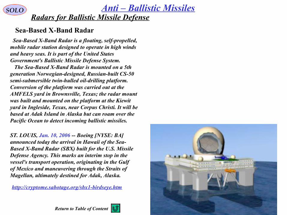
SOLO Anti – Ballistic Missiles
Sea-Based X-Band Radar Sea-Based X-Band Radar is a floating, self-propelled, mobile radar station designed to operate in high winds and heavy seas. It is part of the United States Government's Ballistic Missile Defense System. The Sea-Based X-Band Radar is mounted on a 5th generation Norwegian-designed, Russian-built CS-50 semi-submersible twin-hulled oil-drilling platform. Conversion of the platform was carried out at the AMFELS yard in Brownsville, Texas; the radar mount was built and mounted on the platform at the Kiewit yard in Ingleside, Texas, near Corpus Christi. It will be based at Adak Island in Alaska but can roam over the Pacific Ocean to detect incoming ballistic missiles.
ST. LOUIS, Jan. 10, 2006 -- Boeing [NYSE: BA] announced today the arrival in Hawaii of the Sea-Based X-Band Radar (SBX) built for the U.S. Missile Defense Agency. This marks an interim stop in the vessel's transport operation, originating in the Gulf of Mexico and maneuvering through the Straits of Magellan, ultimately destined for Adak, Alaska.
http://cryptome.sabotage.org/sbx1-birdseye.htm
Radars for Ballistic Missile Defense
Return to Table of Content

Skolnik, M.I., “Introduction to RADAR Systems”, 3th Ed., 2003
Mahafza, B.R.,“Radar Systems Analysis and Design Using MATLAB”,Chapman & Hall, 2000
Skolnik, M.I., “RADAR Handbook”, McGraw Hill, 2nd Ed.,
Stimson, G.W., “Introduction to Airborne RADAR”,
References RADAR Basics
Baton, D.K., “Radar System Analysis And Modeling”,
Long, M.W.,“Radar Reflectivity of Land and Sea”, Artech House,
Baton, D.K., “Modern Radar System Analysis”,
Lacomme, P., Hardange, J.-P., Marchais, J.-C., Normant, E.,“Air and Spaceborne Radar Systems: An Introduction”, SciTech Publishing, 2001
References RADAR Basics

Knott, E.F., Schaeffer, J.F., Tuley, M.T., “Radar Cross Section”, 2nd Ed.,
Knott, E.F., “Radar Cross Measurements”
Kolosov, A., “Over-the-Horizon Radar”, Artech House, 1987Carpentier, M.H., “Principles of Modern Radar Systems”, Artech House, 1988Le Chevalier, F., “Principles of Radar and Sonar Signal Processing”, Artech House, 2002
References

Blackman, S., Popoli, R.,“Design and Analysis of Modern Tracking Systems”, Artech House, 2nd Ed, 1999
Blackman, S.,“Multiple Trget Tracking with Radar Applications”, Artech House, 1986
Bar Shalom, Y., Li, X.R., Kirubarajan, T.,“Estimation with Applications to Tracking and Navigation”,
Bar Shalom, Y.,“Multitarget-Multisensor Tracking :Applications and Advances”, Vol. 2, Artech House, 1992
References
RADAR Basics

Wehner, D.R., “High-Resolution Radar ”, Artech House, 2nd Ed., 1995
Carrara, W.G/. Goodman, R.S., Majewski, R.M.,“Spotlight Synthetic Aperture Radar: Signal Processing Algorithms”, Artech House, 1995
Rihaczek, A.,“Principles of High Resolution Radar”, Artech House, 1996
Soumekh, M, “Synthetic Aperture Radar Signal Processing with MATLAB Algorithms “,John Wiley & Sons, 1999
ReferencesRADAR Basics

Balanis, C.A., “Antenna Theory: Analysis and Design ”, 2nd Ed., John Wiley, 2005
Tsui, J.B., “Microwave Receivers with Electronic Warfare Applications”, John Wiley, 2nd Ed., 2005
Nathanson, F.E.,”Radar Design Principles: Signal Processing and the Environment”, McGraw Hill, 1st Ed., 1969,2nd Ed.,1991
Macfadzean, R.H.M.,” Surface-Based Air Defense Systems Analysis”, Artech House, 1992
References
RADAR Basics

DiFranco, J.V., Rubin, W.L., “Radar Detection”, Artech House, 1981 Barkat, M.,“Signal Detection And Estimation”, Artech House, 1991
Schleher, D.,C., Ed.,“Automatic Detection and Radar Data Processing”, Artech House, 1980
Minkoff, J.R.,“Signals, Noise and Active Sensors: Radar, Sonar, Laser Radar ” , John Wiley & Sons, 1992
References
RADAR Basics
Barton, D.K., “Radars Volume 4: Radar Resolution and Multipath Effects ”, Artech House, 1975
Barton, D.K., “Radars Volume 2: Radar Equation”, Artech House, 1974
Barton, D.K., “Radars Volume 1: Monopulse Radar”, Artech House, 1977
Barton, D.K., “Radars Volume 3: Pulse Compression”, Artech House, 1974
References
RADAR Basics

Barton, D.K., “Radars Volume 7: CW and Doppler”, Artech House, 1978
Barton, D.K., “Radars Volume 5: Radar Clutter”, Artech House, 1974
Barton, D.K., “Radars Volume 6: Freqency Agility and Diversity”, Artech House, 1974
References
RADAR Basics

Morris, G., “Airborne Pulsed Doppler Radar”, Artech House, 1996
Scheer, J.A., Kurtz, J.L.,Ed., “Coherent Radar Performance Estimation” , Artech House,1993
Jenn, D., “Radar and Laser Cross Section Engineering: Lessons Learned from the Aviation Industry”, American Institute of Aeronautics & Astronautics, 2005
Nitzberg, R.,”Adaptive Signal Processing for Radar”, Artech House, 1991Currie, N.C.,Ed., “Techniques of Radar Reflectivity Measurement, Atech House, 1984
References
RADAR Basics

Hovanessian, S.A.,“Radar Detection and Tracking Systems” , Artech House,1973
Hovanessian, S.A.,“Radar System Design and Analysis” , Artech House,1984
Levanon, N.,“Radar Principles” , John Wiley & Sons, 1988 Peebbles, P.Z., “Radar Principles “, John Wiley & Sons, 1998
References
RADAR Basics

Brookner, E.,“Tracking and the Kalman Filter Made Easy” , John Wiley & Sons, 1998
Brookner, E., Ed., “Radar Technology” , Artech HouseCook, C.C., Bernfeld, M., “Radar Signals: An Introduction to Theory and Application”,
Artech House, 1993Schleher, D.C.,“MTI and Pulsed Doppler Radar”, Artech House, 1991
References
RADAR Basics

Galati, G., Ed.,“Advanced Radar Techniques and Systems”, IEE Radar, Sonar, Navigation and Avionics Series 4, Peter Peregrinus Ltd., 1993
Sabatini, S., Tarantino, M., “Multifunction Array Radar: System Design and Analysis”, Artech House, 1994
Ulaby, F.T., Fung, A.K., Moore, R.K., “Microwave Remote Sensing, Active and Passive: Radar Remote Sensing and Surface Scattering and Emission Theory”, Vol. 2, Artech House, 1982
Farina, A., “Antenna-Based Signal Processing Techniques for Radar Systems”, Artech House, 1992
ReferencesRADAR Basics
Barton, D.K., Leonov, A.I., Leonov, S.A., Morozov, A.I., Hamilton, P.C., “Radar Technology Encyclopedia ” , Artech House, 1997
Jelalian, A.V.,“Laser Radar Systems”, Artech House, 1991
Edde, B., “Fundamentals of Radar: Self Study Course”, IEEE, 1999
Blake, L.V., “Radar Range Performance Analysis”, Artech House, 1986
References RADAR Basics

Zmuda, H., Touglian, E.N., “Photonic Aspects of Modern Radar ” , Artech House, 1994
Neri, F., “Introduction to Electronic Defense Systems”, SciTech Publishing, Incorporated,2006
ReferencesRADAR Basics

SOLO
References
RADAR Basics
1. S. Hermelin, “My RADAR Reference Books”,
2. S. Hermelin, “Electromagnetic Waves & Photons”,
3. S. Hermelin“Short History of Radar Beginnings”,
4. S. Hermelin “Airborne Radars1”, . “Airborne Radars2”,
. “Airborne Radars Examples2”,
. “Airborne Radars Examples1”,
5. S .Hermelin, “Pulse Radar Doppler Seeker”,

SOLO
References
S. Hermelin, “Range & Doppler Measurements in RADAR Systems”,
RADAR Basics
S. Hermelin, “Clutter Models”,
Return to Table of Content
S. Hermelin, “Radar Signal Processing”,
S. Hermelin , “Fourier Transforms in Radar”,
S. Hermelin, “Matched Filters and Ambiguity Functions for Radar Signals”,
S. Hermelin, “Pulse Compression Waveforms”,
S. Hermelin, “Detection Decisions”,
Georgia Tech Lectures in RADAR

January 15, 2015 215
SOLO
TechnionIsraeli Institute of Technology
1964 – 1968 BSc EE1968 – 1971 MSc EE
Israeli Air Force1970 – 1974
RAFAELIsraeli Armament Development Authority
1974 –
Stanford University1983 – 1986 PhD AA

http://www.radartutorial.eu

SOLO

SOLO
Formation of Standing Waves
Standing wave in a string (both ends clamped).
Formation of standing wave through reflection of a sinusoidal wave at a fixed end.
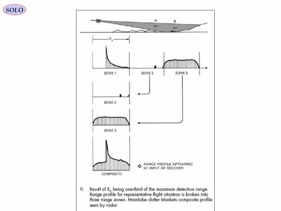
SOLO

SOLO

SOLO
“Introduction to Airborne Radar”, George W. Stimson, 2nd Ed. Scitech Publishing

CW semi-active seeker
MISSILE SIGNALS-AMPLITUDEMISSILE SIGNALS-AMPLITUDEvs FREQUENCYvs FREQUENCY
SOLO

CW semi-active seekerSOLO
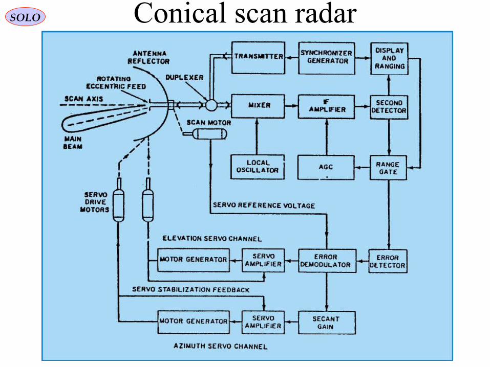
Conical scan radarSOLO

SOLO

Pulse Radar Parameters
Transmitted Signal
Tr
Tp
F0
Tr – Pulse Repetition Interval (PRI)Tp – Transmitted Pulse WidthF0 – Transmitted RF frequencyPp – RF peak power D.C – Duty Cycle = Tp/Tr
Pav – RF average power = Pp*D.C

Pulse Doppler Radar – Clutter
Altitude return
AntennaMain Beam
AntennaSide Lobes
Ground
Target
Power
Frequency
Altitude Side lobe
Main Lobe
Incoming TargetReceding Target
λVc2
Doppler
Range
Radar Altitude
Vradar
Side lobe Clutter
Main Lobe Clutter
Incoming Targets
Receding Targets
CrossingTargets
Noise limitedClutter limited

Pulse Doppler Radar – Clutter
Clutter Cross Section in Doppler Cell
clutterat Gain Antenna )G(
tcoefficien Reflection
widthgate Range R
clutter todirection fligh between Angle
VelocityRadar V
Length WavedTransmitte
thfilter wid FFT B
clutter toRange
)()sin2
(
a
0
g
0
==
======
=
θσ
θ
λ
θσθ
λσ
R
GRV
RB ag2 cos
D
Vf
θλ
=
2 cosD
BB
f V
λθ
=

Detection of Radar SignalsSwerling Models
Case 1The echo received from a target on any look is constant but are independent (uncorrelated) from look to lookThe probability-density function for the RCS:
nsfluctuatio target allover RCS average theis
)exp(1
)(
av
avav
p
σσσ
σσ −=
Case 2The probability-density function for the RCS is same as for Case 1, but the fluctuations are more rapidCases 1 and Case 2 apply to a target consisting of many independent scatterers equal in RCS - Aircrafts

Probability Density Swerling 1

Detection of Radar SignalsSwerling Models
Case 3The fluctuation is assumed to independent from look to look as in Case 1, but the probability density function is given by
)2
exp(4
)(2
avav
pσ
σσ
σσ −=Case 4The probability-density function for the RCS is same as for Case 2, but the fluctuations are more rapidCase 3 and Case 4 apply to a target that can be represented as one large reflector together with other small reflectors - Ships
In all the above cases the RCS value in the radar equation is the average RCS.The probability of detecting a given RCS can be calculated

Probability Density Swerling 3

Detection of Radar SignalsNoise and False Alarm
The noise is assumed to be Gaussian with probability density function
noise theof valuesquare-mean theis
dv vand v valueebetween th v voltagenoise thefinding ofy probabilit theis )(
)2
exp(2
1)(
0
0
2
0
ψ
ψπψ+
−=
dvvp
dvv
dvvp
The probability that the noise envelope will exceed the voltage threshold VT is Pfa
)2
exp(0
2
ψT
fa
VP −=

Detection of Radar Signals
Integration of pulse trains
The probability of detection for M-out-of-N:
∑=
−−−
=N
Mj
jNd
jdd pp
jNj
NP )1(
)!(!
!
Pd probability of single detection
And the probability of false alarm
∑=
−−−
=N
Mj
jNn
jnn pp
jNj
NP )1(
)!(!
!
Pn probability of false alarm in single detection

•Extraction of Information• PRF selection guide lines:
– Incoming targets – High PRF• No Doppler ambiguity• Range ambiguity
– Receding targets – Medium PRF• Range and Doppler ambiguity
– Crossing targets – low PRF given target and main lobe clutter are not co-range – other wise no detection
• No range ambiguity• Doppler ambiguity

Extraction of Informationλ
cVPRF 4≥

Extraction of InformationThe Range coverage equals PRI – 2*Pulse_width + recovery timeThe pulse width is defined by PRI and maximum available duty cycle
Example: PRF = 100 KHz; Duty cycle 10%
PRI = 1/PRF = 10 µsec= 1500 meters Maximum pulse width = 150 meters Maximum range coverage 1500 – 300 = 1200 meters.In this example if range uncertainty is smaller than 1200 meters, one PRF is suffice.Otherwise a set of PRF’s must be selected to cover the uncertainty.
All targets ranges above PRI are folded within PRI – range ambiguity

Extraction of InformationTarget range = N PRI + R1
Where R1 = Target Range within PRI
N = number of folds 0…N
)(
1
PRI
RfixN
PRIRR
T
T
=
⊗=
ExampleRT=12,300 m PRI = 1500 m
N = fix(12300/1500) = 8 R1= 12300-1500*8=300 meters

Extraction of Information
PRI1
PRI2
R1
R2
Target

Extraction of InformationResolving range ambiguity
Use at least 2 PRF’s so RT = N PRI1+R1 = M PRI2 + R2
PRF1 and PRF2 are derived from basic clock so K1*clock= PRF1 and K2*clock=PRF2Maximum unambiguous range is 1/ K1*K2*clock.Where K1 and K2 are prime numbers.
Example Clock = 20 KHz K1=6 K2=7 PRF1 = 120 KHz PRF2 = 140 KHz PRI1= 1250 m PRI2~ 1070 m R1= 950 m R2= 70 m True range = 7*1250+950= 9*1070+70=9700 m N= 7 M=9
Same applies for resolving the Doppler ambiguity.

Extraction of InformationRange Tracking
TargetAmplitude
Range Sampling
Range Gate
CFAR ThresholdE1
E2
E3
R11 R12 R13
∑++=3,2,1
313212111 rangeTarget E
ERERER
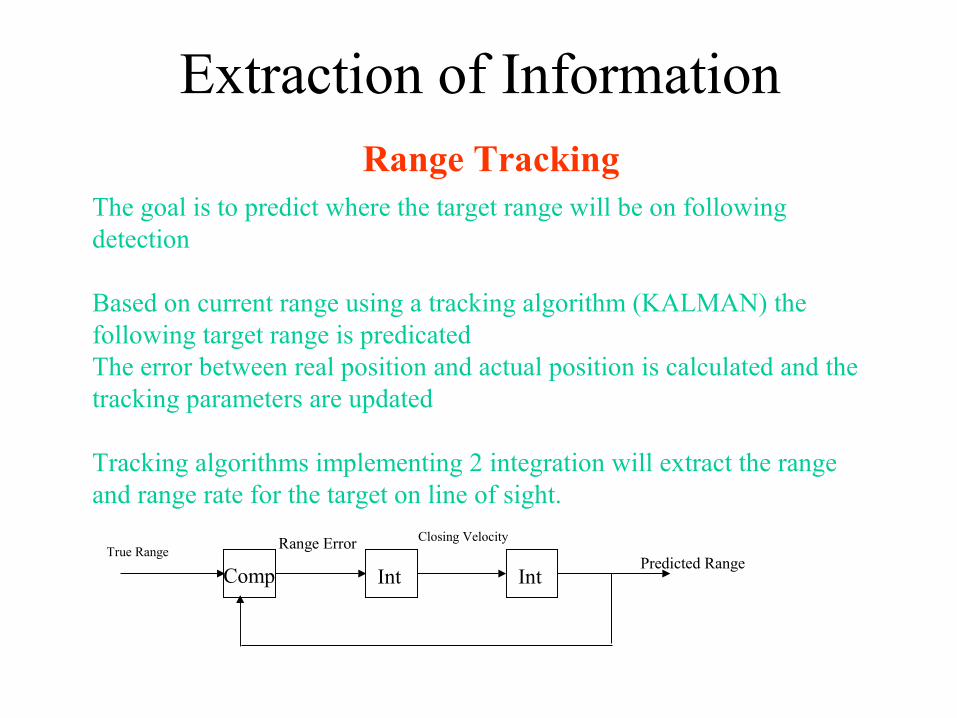
Extraction of InformationRange Tracking
The goal is to predict where the target range will be on following detection
Based on current range using a tracking algorithm (KALMAN) the following target range is predicatedThe error between real position and actual position is calculated and the tracking parameters are updated
Tracking algorithms implementing 2 integration will extract the range and range rate for the target on line of sight.
Comp Int IntTrue Range
Predicted Range
Closing VelocityRange Error
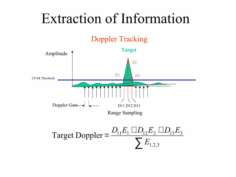
Extraction of InformationDoppler Tracking
TargetAmplitude
Range Sampling
Doppler Gate
CFAR ThresholdE1
E2
E3
D11 D12 D13
∑++=3,2,1
313212111 Doppler Target E
EDEDED

Doppler Tracking
The goal is to predict where the target Doppler will be on following detection
Based on current Doppler using a tracking algorithm (KALMAN) the following target Doppler is predicatedThe error between real Doppler and actual Doppler is calculated and the tracking parameters are updated
Tracking algorithms implementing 1 integration will extract the Doppler on line of sight.
Comp IntTrue Doppler Predicted DopplerDoppler Error
Extraction of Information

Extraction of InformationAngular Information
The Monopulse concept:
L
θ
θ
L sinθ
The path difference between the signals as received at each lobe is L sin θ The phase difference φ for a wavelength λ:
λαπφ sin
2l=
The outputs from lobes are added and subtracted as vectors
)2
sin(
)2
cos(
φ
φ
∆
Σ
=∆
=Σ
K
KSUM
Difference

Extraction of InformationSum and Difference patterns
Sum
Difference
λαπφ sin
2l=
Output level

Extraction of Information
Σ∆=Σ∆=
and between angle
))sin(tan(
ϕ
ϕaError
Error output
Target angle

Interference
Multipath
Direct wave
Reflected
wave RadarTarget
Image
Tx Ri Rt
Reflecting Surface
t
HtHr
R

InterferenceMultipath
Phase difference corresponding to the path-length difference
R
HH rtd
22
λπϕ =
The ratio of power incident on the target compared to a target in free space (no multipath)
)2
(sin 4
R
HHKP tr
r λπ=
So the power at a specific ranges can be decrease to zero – fading effect.Additional effect is an angular tracking error due to the presence of image

Interference
ECM
The Signal to Jammer ration is Prt/Prj
4
2
4 t
j
jrjj
rtt
rj
rt
R
R
GGP
GGP
P
P
πσ=
Gjr = is the radar antenna gain in the direction of jammerRj = range radar to jammerRt = range radar to targetPj = is the jammer power within radar bandwith

Interference
• Jamming techniques– ON-OFF– RGPO– VGPO– Towed– Expandable– Chaff– Cross-eye– Inverse gain– others
ECM

SOLO

SOLO

SOLO
Figure: estimating of the angular position
Monopulse Concept
Monopulse radars find their origin in tracking systems. Since the late 1970s, the principle of monopulse has been adapted to suit PSR and SSR systems and is in common
operational use world-wide today
A target will be seen by a radar from the moment it enters the main antenna beam or from the moment it is illuminated by the transmitted radar antenna beam. A search radar always makes an error in the determination of the direction of the target because it makes the assumption that the target is situated in the direction of the axis of the main beam of the antenna. This error is of the order of the beam width of the main antenna beam.

SOLO

http://atcsl.tripod.com/radar_theory.htm

AV
TxV
R
Airborne Radar Vehicle
TsV
TV
Ground Moving Target
r∆
r∆
Range Resolution
=∆
2
81.1 c
BWr
=∆
2
81.1 λT
r
Doppler Resolution
( )( )( ) ( ) ( )trtVRtr
ttVRRtr
VVV
Ts
Ts
TsTxA
/
2
:
2
222
222
γ
γ
γ
+=
++=
+−=
Significant range walkwith large BW and T
Significant Doppler walkwith large T c - speed of light
BW – bandwidthλ - wavelengthT - CPI timeVA - aircraft velocityVT - target velocityR - stand-off Range
Long CPI can lead to target doppler walk or smearing.The degree of smearing is a function of λ2.
Mechanism for Moving Target Smearing

Range & Doppler Measurements in RADAR SystemsSOLO
Chinese Remainder Theorem The original form of the theorem, contained in a third-century AD book by Chinese mathematician Sun Tzu and later republished in a 1247 book by Qin Jiushao.
Suppose n1, n2, …, nk are integers which are pairwise coprime. Then, for any given integers a1,a2, …, ak, there exists an integer x solving the system
1 1 1 1 1
2 2 2 2 2
1 2
0
0
0
, , , integersk k k k k
k
x n t a n a
x n t a n a
x n t a n a
t t t are
≡ + > >≡ + > >
≡ + > >L L L L L
L
or in modern notation
( )mod 1,2, ,i ix a n i k≡ = L ai is the reminder of x : ni
x

Range & Doppler Measurements in RADAR SystemsSOLO
Chinese Remainder Theorem (continue – 1)
A Constructive Solution to Find x
( )mod 1,2, ,i ix a n i k≡ = L
x
Define 1 2: kN n n n= L
For each i, ni and N/ni are coprime.
Using the extended Eulerian algorithm we can therefore find integers ri and si such that
( )/ 1i i i irn s N n+ =Define
Therefore ei divided by ni has the remainder 1 and divided by nj (j≠i) has the remainder 0,because of the definition of N.
( ): / 1i i i i ie s N n rn= = −
( ) ( )1 mod 0 modi i i je n and e n i j= = ∀ ≠Because of this the solution is of the form
1
k
i ii
x a e=
= ∑ But also ( )1
modk
i ii
a e x N=
=∑

Range & Doppler Measurements in RADAR SystemsSOLO
Chinese Remainder Theorem (continue – 2)
A Constructive Solution to Find x (Example)
( )mod 1,2, ,i ix a n i k≡ = L
1 2 3: 60N n n n= × =
( )( )( )
2 mod 3 ,
3 mod 4 ,
1 mod 5 .
x
x
x
≡
≡
≡1 2 33, 4, 5n n n= = =
1 2 3/ 20, / 15, / 12N n N n N n= = =
( )
11 11
/
13 3 2 20 1sn N n
r
− + = ÷
( )
2 2 22
/
11 4 3 15 1n s N n
r
− + = ÷
( ) ( )
33
3 3/
5 5 2 12 1N nn
r s
+ − = ÷
( ): /i i ie s N n= ( )1 : 2 20 40e = = ( )2 : 3 15 45e = = ( )3 : 2 12 24e = − = −
1 2 32, 3, 1a a a= = =
( )1 1 2 2 3 3 2 40 3 45 1 24 191x a e a e a e= + + = × + × + × − =
Check:
191 63 3 2 47 4 3 38 5 1= × + = × + = × +
( )/ 1i i i irn s N n+ =Find ri and si such that:
Compute:
Therefore:
and ( )11 191 11 mod 60x N= ¬ = =
11 3 3 2 2 4 3 2 5 1= × + = × + = × +

Range & Doppler Measurements in RADAR SystemsSOLO
The transmitted RADAR RF Signal is:
( ) ( ) ( )[ ]ttftEtEt 0000 2cos ϕπ +=E0 – amplitude of the signal
f0 – RF frequency of the signal φ0 –phase of the signal (possible modulated)
The returned signal is delayed by the time that takes to signal to reach the target and toreturn back to the receiver. Since the electromagnetic waves travel with the speed of lightc (much greater then RADAR andTarget velocities), the received signal is delayed by
c
RRtd
21 +≅
The received signal is: ( ) ( ) ( ) ( )[ ] ( )tnoisettttftEtE ddr +−+−= ϕπα 000 2cos
To retrieve the range (and range-rate) information from the received signal thetransmitted signal must be modulated in Amplitude or/and Frequency or/and Phase.
ά < 1 represents the attenuation of the signal

Range & Doppler Measurements in RADAR SystemsSOLO
The received signal is:
( ) ( ) ( ) ( )[ ] ( )
( ) ( ) ( )tnoisec
RRtRRtftE
tnoisettttftEtE
fc
ddr
+
+−++−=
+−+−==
2121
0000
/
000
22cos
2cos
00
ϕλππα
ϕπαλ
If we consider only (c = speed of light) then the frequency of the electromagneticwave that reaches the receiver is given by:
ctd
Rd <<
+
−≈
+
+−=
+−+
+−=
c
td
Rd
td
Rd
f
c
tdRd
tdRd
ud
dff
c
RRt
c
RRtf
td
df
21
0
21
0~
00
21210
1
2
1
22
1
ϕπ
ϕππ
λ
+
−=td
RdtdRd
fd
21
is the doppler frequency shift at the receiver
Christian Johann Doppler first observed the effect in acoustics.

TV
1R
If the Radar Receiver is at a distance R1 from the Target and the Receiver isat a distance R2 from the Target, then the frequency of the carrier wave at the Receiver is:
λλ
−
−=td
RdtdRd
ff
21
0
( ) 111111 // RRVVRRR
td
RdET
⋅−=⋅= is the relative velocity between the Target and the Radar source along the line of sight between them
( ) 222222 // RRVVRRR
td
RdMT
⋅−=⋅= is the relative velocity between the Target and the Receiver along the line of sight between them
SOLO Doppler Frequency Shift
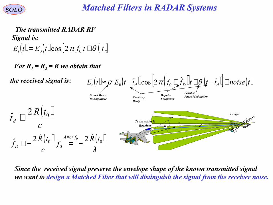
Matched Filters in RADAR SystemsSOLO
α MV R
EVTarget
Transmitter &Receiver
The transmitted RADAR RF Signal is:
( ) ( ) ( )[ ]ttftEtEt θπ += 00 2cos
( )c
tRtd
02ˆ ≅
Since the received signal preserve the envelope shape of the known transmitted signalwe want to design a Matched Filter that will distinguish the signal from the receiver noise.
the received signal is: ( ) ( ) ( ) ( )[ ] ( )tnoisetttffttEtE dDdr +−++−≈ ˆˆ2cosˆ00 θπα
Scaled DownIn Amplitude Two-Way
Delay
Possible Phase ModulationDoppler
Frequency
( ) ( )λ
λ0
/
00 22ˆ 0 tR
fc
tRf
fc
D
−=−≅
=
For R1 = R2 = R we obtain that

SOLO Review of Probability
Exponential Distribution
( ) ( )
<≥−
=00
0exp;
x
xxxp
λλλ
( ) ( )
( )( ) ( )
λλλ
λλ
λλ
1expexp
exp
00exp
0
=−+−−=
−=
∫
∫∞
∞=
−=
∞
dxxxx
dxxxxE
xu
dxxdv
( ) ( ) ( )2
22 1
λ=−= xExExVar
( ) ( )[ ] ( ) ( )
( )[ ]1
0
0
1exp
expexpexp
−∞
∞
−=−
−=
−==Φ ∫
λωλω
λωλ
λλωωω
jxj
j
dxxxjxjEX
Probability Density Functions
Cumulative Distribution Function
Mean Value
Variance
Moment Generating Function
( ) ( ) ( )
<≥−−
=−= ∫∞− 00
0exp1exp;
x
xxdxxxP
x λλλλ
( ) ( )2
0
2
222 2
λω ω
=Φ==d
djxE X
Distributionsexamples
Table of Content

SOLO Review of Probability
Chi-square Distribution
( )( )
( )( ) ( )
<
≥−Γ=
−
00
02/exp2/
2/1;
2/2
2/
x
xxxkkxp
k
k
( ) kxE =
( ) kxVar 2=
( ) ( )[ ]( ) 2/21
expk
X
j
xjE−−=
=Φ
ω
ωω
Probability Density Functions
Cumulative Distribution Function
Mean Value
Variance Moment Generating Function
( )( )
( )
<
≥Γ=
00
02/
2/,2/
;
x
xk
xk
kxP
γ
Γ is the gamma function ( ) ( )∫∞
− −=Γ0
1 exp dttta a
( ) ( )∫ −= −x
a dtttxa0
1 exp,γγ is the incomplete gamma function
Distributionsexamples

SOLO Review of ProbabilityStudent’s t-Distribution
( ) ( )[ ]( ) ( ) ( ) 2/12 /12/
2/1; ++Γ
+Γ= νννπννν
xxp
( )
=>
=1
10
νν
undefinedxE
( ) ( )∞
>−=
otherwisexVar
22/ ννν
Probability Density Functions
Cumulative Distribution Function
Mean Value
Variance
Moment Generating Function not defined
( ) ( )[ ]( ) ∑
∞
=
−
+
Γ+Γ+=
0
2
!2
3
2
1
2
1
2/
2/1
2
1;
n
n
n
nn
n
x
xxP
νν
ννπνν
Γ is the gamma function ( ) ( )∫∞
− −=Γ0
1 exp dttta a
( ) ( ) ( ) ( )121: −+++= naaaaa n L
It get his name after W.S. Gosset that wrote under pseudonym “Student”
William Sealey Gosset
1876 - 1937
Distributionsexamples
Table of Content

SOLO Review of Probability
Uniform Distribution (Continuous)
( )
>>
≤≤−=
bxxa
bxaabbaxp
0
1,;
( )2
baxE
+=
( ) ( )12
2abxVar
−=
( ) ( )[ ]( ) ( )
( )abj
ajbj
xjE
−−=
=Φ
ωωω
ωωexpexp
exp
Probability Density Functions
Cumulative Distribution Function
Mean Value
Variance
Moment Generating Function
( )
>
≤≤−−
>
=
bx
bxaab
ax
xa
baxP
1
0
,;
Distributionsexamples
Moments
Table of Content

SOLO Review of Probability
Rayleigh Distribution
( )2
2
2
2exp
;σ
σσ
−
=
xx
xp
( )2
πσ=xE
( ) 2
2
4 σπ−=xVar
Probability Density Functions
Cumulative Distribution Function
Mean Value
Variance
Moment Generating Function
( )
−−=
2
2
2exp1;
σσ x
xP
( ) ( )
−
−−=Φ jerfi
222/exp1 22 σωπσωσωω
John William Strutt
Lord Rayleigh
(1842-1919)
Distributionsexamples
Moments
Rayleigh Distribution is the chi-distribution with k=2( ) ( ) ( )
( ) ( )kk
k
k
k
k
k Uk
pk
χσ
χσ
χχ
−
Γ=
−−−
Χ 2
212/2
2exp
2/
2/1

SOLO Review of Probability
Rayleigh Distribution
Given X and Y, two independent gaussian random variables, with zero means and thesame variances σ2
Example of Rayleigh Distribution
( )
+−=2
22
2 2exp
2
1,
σσπyx
yxpXY
find the distributions of R and Θ given by: ( )XYYXR /tan& 122 −=Θ+=
( ) ( )
( ) ( ) θθσπ
θσ
σπσθθ
dprdrpdrdrr
ydxdyxydxdyxpdrdrp
r
XYR
Θ
Θ
=
−=
+−==
22
2
22
22
22exp
22exp,,
where:( ) πθ
πθ 20
2
1 ≤≤=Θp
( ) 02
exp2
2
2≥
−= r
rrrpr σσ
Uniform Distribution
Rayleigh Distribution
Solution
Table of Content
x
y
rθ

SOLO Review of Probability
Rice Distribution
( )
+−=
202
2
22
2exp
,;σσ
σσ vx
I
vxx
vxp
( )2
πσ=xE
( ) 2
2
4 σπ−=xVar
Probability Density Functions
Cumulative Distribution Function
Mean Value
Variance Moment Generating Function
( )
−−=
2
2
2exp1;
σσ x
xP
( ) ( )
−
−−=Φ jerfi
222/exp1 22 σωπσωσωω
Stuart Arthur Rice1889 - 1969
Distributionsexamples
where:
( ) ( )∫
−=
π
ϕσ
ϕπσ
2
0220 '
2
'cosexp
2
1d
vxvxI

SOLO Review of Probability
Rice Distribution
The Rice Distribution applies to the statistics of the envelope of the output of a bandpassfilter consisting of signal plus noise.
Example of Rice Distribution
( ) ( ) ( ) ( ) ( ) ( ) ( )( )[ ] ( ) ( )[ ] ( )tAtntAtn
ttnttntAtnts
SC
SC
00
000
sinsincoscos
sincoscos
ωϕωϕωωϕω
−++=+++=+
X = nC (t) and Y = nS (t) are gaussian random variables, with zero mean and the samevariances σ2 and φ is the unknown but constant signal phase.
Define the output envelope R and phase Θ:
( )[ ] ( )[ ]( )[ ] ( )[ ] ϕϕ
ϕϕ
cos/sintan
sincos1
22
AtnAtn
AtnAtnR
CS
SC
+−=Θ
−++=−
( ) ( ) ( ) ( )
( )222
22
22
2
2
2
22
cosexp
2exp
22
sinexp
2
cosexp,,
σπθ
σθϕ
σ
σπσϕ
σϕθθ
drdrrAAr
ydxdAyAxydxdyxpdrdrp XYR
+−
+−=
−−
+−==Θ
Solution
( ) ( ) ( ) ( )∫∫ +
+−
+−== Θ
ππ
θϕσ
θϕσπσ
θθ2
0222
222
0 2
cosexp
22exp, d
rArArdrprp RR

SOLO Review of Probability
Rice Distribution
Example of Rice Distribution (continue – 1)
( ) ( ) ( ) ( )∫∫
−
+−== Θ
ππ
ϕσ
ϕπσσ
θθ2
022
22
2
2
0
'2
'cosexp
2
1
2exp, d
rAArrdrprp RR
where:
( ) ( )∫
−=
π
ϕσ
ϕπσ
2
0220 '
2
'cosexp
2
1d
rAArI
is the zero-order modified Bessel function of the first kind
( )
+−=202
22
2 2exp,;
σσσσ Ar
IArr
ArpR Rice Distribution
Since I0 (0) = 1, if in the Rice Distribution we take A = 0 we obtain:
Rayleigh Distribution( )
−==
2
2
2 2exp,0;
σσσ rr
ArpR
Table of Content
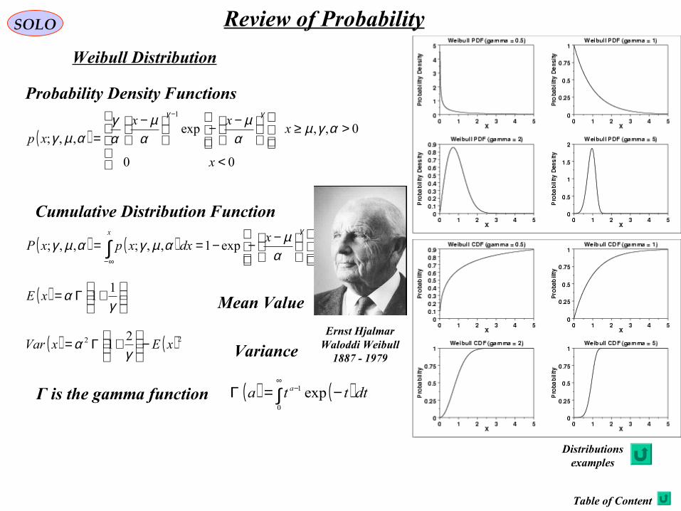
SOLO Review of Probability
Weibull Distribution
( )
<
>≥
−−
−
=
−
00
0,,exp,,;
1
x
xxx
xpαγµ
αµ
αµ
αγ
αµγ
γγ
( ) ( )
−−−== ∫
∞−
γ
αµαµγαµγ x
dxxpxPx
exp1,,;,,;
( )
+Γ=
γα 1
1xE
Γ is the gamma function ( ) ( )∫∞
− −=Γ0
1 exp dttta a
Ernst HjalmarWaloddi Weibull
1887 - 1979
Probability Density Functions
Cumulative Distribution Function
Mean Value
Variance( ) ( ) 22 21 xExVar −
+Γ=
γα
Distributionsexamples
Table of Content