1. probability models in electrical and computer...

Notes and figures are based on or taken from materials in the textbook: Alberto Leon-Garcia, “Probability, Statistics, and Random Processes For Electrical Engineering, 3rd ed.”, Pearson Prentice Hall, 2008, ISBN: 013-147122-8.

1 of 17

1. Probability Models in Electrical and Computer Engineering

Electrical and computer engineers have played a central role in the design of modern information and communications systems. These highly successful systems work reliably and predictably in highly variable and chaotic environments:

• Wireless communication networks provide voice and data communications to mobile users in severe interference environments.

• The vast majority of media signals, voice, audio, images, and video are processed digitally.

• Huge Web server farms deliver vast amounts of highly specific information to users.

Because of these successes, designers today face even greater challenges. The systems they build are unprecedented in scale and the chaotic environments in which they must operate are untrodden territory

Web information is created and posted at an accelerating rate; future search applications must become more discerning to extract the required response from a vast ocean of information.

Information-age scoundrels hijack computers and exploit these for illicit purposes, so methods are needed to identify and contain these threats.

Machine learning systems must move beyond browsing and purchasing applications to real-time monitoring of health and the environment.

Massively distributed systems in the form of peer-to-peer and grid computing communities have emerged and changed the nature of media delivery, gaming, and social interaction; yet we do not understand or know how to control and manage such systems.:

Probability models are one of the tools that enable the designer to make sense out of the chaos and to successfully build systems that are efficient, reliable, and cost effective. This book is an introduction to the theory underlying probability models as well as to the basic techniques used in the development of such models.


2 of 17

1.1 Mathematical Models as Tools in Analysis and Design

Model

An approximate representation of a physical situation. A model attempts to explain observed behavior using a set of simple and understandable rules.

These rules can be used to predict the outcome of experiments involving the given physical situation.

Mathematical models

Used when the observational phenomenon has measurable properties.

A mathematical model consists of a set of assumptions about how a system or physical process works. These assumptions are stated in the form of mathematical relations involving the important parameters and variables of the system.

The conditions under which an experiment involving the system is carried out determine the “givens” in the mathematical relations, and the solution of these relations allows us to predict the measurements that would be obtained if the experiment were performed.

Computer simulation model

Consists of a computer program that simulates or mimics the dynamics of a system.

Incorporated into the program are instructions that “measure” the relevant performance parameters.

In general, simulation models are capable of representing systems in greater detail than mathematical models. However, they tend to be less flexible and usually require more computation time than mathematical models..


3 of 17

A flow chart of the modeling process

1.2 Deterministic Models and Probability Models – Some Definitions

Deterministic models (determining a result)

The conditions under which an experiment is carried out determine the exact outcome of the experiment.

In deterministic mathematical models, the solution of a set of mathematical equations specifies the exact outcome of the experiment.

Circuit theory is an example of a deterministic mathematical model

Probability models (incorporate a random variable or process)

We define a random experiment to be an experiment in which the outcome varies in an unpredictable fashion when the experiment is repeated under the same conditions.

Deterministic models are not appropriate for random experiments since they predict the same outcome for each repetition of an experiment.

“Games of chance” are based on probability and probabilistic models of performance.


4 of 17

Experiment

An experiment is some action that results in an outcome.

A random experiment is one in which the outcome is uncertain before the experiment is performed.

Possible Outcomes

A description of all possible experimental outcomes.

The set of possible outcomes may be discrete or form a continuum.

Sample space

The set containing all possible outcomes.

Trials

The single performance of a well-defined experiment.

Event

An elementary event is one for which there is only one outcome.

A composite event is one for which the desired result can be achieved in multiple ways. Multiple outcomes result in the event described.

In order to be useful, a model must enable us to make predictions about the future behavior of a system, and in order to be predictable, a phenomenon must exhibit regularity in its behavior.

Statistical Regularity

Many probability models in engineering are based on the fact that averages obtained in long sequences of repetitions (trials) of random experiments consistently yield approximately the same value.


5 of 17

The balls in an urn example:

Suppose a ball is selected from an urn containing three identical balls, labeled 0, 1, and 2.The urn is first shaken to randomize the position of the balls, and a ball is then selected. The number of the ball is noted, and the ball is then returned to the urn.

The outcome of this experiment is a number from the set 2,1,0S . We call the set S of all possible outcomes the sample space.

Figure 1.2 shows the outcomes in 100 repetitions (trials) of a computer simulation of this urn experiment. It is clear that the outcome of this experiment cannot consistently be predicted correctly.

Relative Frequency

When an experiment is repeated a number of times, n, under identical conditions (like the balls in an urn experiment) the number of times each possible outcome occurs can be identified, such as N0(n), N1(n), and N2 (n) for the three balls. Then the relative frequency of each outcome can be defined as

n

nNnf k

k

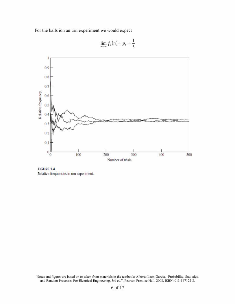
If the experiment has statistical regularity, the relative frequency should converge to a constant probability as the number of trials becomes very large, or

kkn

pnf

lim


6 of 17

For the balls ion an urn experiment we would expect

3

1lim

kkn

pnf


7 of 17

1.3.2 Properties of Relative Frequency

For a random experiment with K possible outcomes, we can identify:

The sample space: KS ,,3,2,1

The number of occurrences of each outcome

KkfornnN k ,.3,2,1,0

The relative frequency n

nNnf k

k

where 10 nfk

Properties:

The sum of the number of occurrences of each outcome is n

nnNK

kk

1

The sum of the relative frequencies is 1

111

K

kk

K

k

k nfn

nN

The balls in an urn example:

A composite event based on this experiment can be defined developed based on the primitive functions. For example, determining the composite event that “the ball selected is even” … that is either a 0 or a 2.

The relative frequency of the composite event is then

nNnNnNeven 20

nNnNodd 1

and the relative frequency is

nfnfnfeven 20

nfnfodd 1


8 of 17

1.3.3 The Axiomatic Approach to a Theory of Probability

First of all, it is not clear when and in what mathematical sense the limit in Eq. (1.2) exists.

Second, we can never perform an experiment an infinite number of times, so we can never know the probabilities pk exactly.

Finally, the use of relative frequency to define probability would rule out the applicability of probability theory to situations in which an experiment cannot be repeated.

Thus it makes practical sense to develop a mathematical theory of probability that is not tied to any particular application or to any particular notion of what probability means.

The modern theory of probability begins with a construction of a set of axioms that specify that probability assignments must satisfy these properties. It supposes that:

(1) a random experiment has been defined, and a set S of all possible outcomes has been identified;

(2) a class of subsets of S called events has been specified; and

(3) each event A has been assigned a number, P[A], in such a way that the following axioms are satisfied:

1. 10 AP

2. 1SP

3. If A and B are events in S that cannot occur simultaneously, then BPAPBorAP


9 of 17

MATLAB Marble Examples from ECE 3800:

A bag of marbles: 3-blue, 2-red, one-yellow Objects: Marbles Attributes: Color (Blue, Red, Yellow) Experiment: Draw one marble, with replacement Sample Space: {B, R, Y} Probability (relative frequency method)

The probability for each possible event in the sample space is ….

Event Probability

Blue 3/6

Red 2/6

Yellow 1/6

Total 6/6

Experiment 2: A bag of marbles, draw 2 •Experiment: Draw one marble, replace, draw a second marble.

“with replacement” •Sample Space: {BB, BR, BY, RR, RB, RY, YB, YR, YY}

The probability for each possible event in the sample space is ….

Therefore 1st-rows\2nd-col

Blue Red Yellow

Blue

36

9

6

3

6

3

36

6

6

2

6

3

36

3

6

1

6

3

Red

36

6

6

3

6

2

36

4

6

2

6

2

36

2

6

1

6

2

Yellow

36

3

6

3

6

1

36

2

6

2

6

1

36

1

6

1

6

1


10 of 17

Experiment 3: A bag of marbles, draw 2 without replacement •Experiment: Draw two marbles, without replacement •Sample Space: {BB, BR, BY, RR, RB, RY, YB, YR}

The probability for each possible event in the sample space is …. 1st-

rows\2nd-col

Blue Red Yellow 1st

Marble

Blue 30

6

5

2

6

3

30

6

5

2

6

3

30

3

5

1

6

3

6

3

Red 30

6

5

3

6

2

30

2

5

1

6

2

30

2

5

1

6

2

6

2

Yellow 30

3

5

3

6

1

30

2

5

2

6

1

30

0

5

0

6

1

6

1

2nd Marble 6

3

6

2

6

1

6

6


11 of 17

1.4 A Detailed Example: A Packet Voice Transmission System

The presentation intentionally draws upon your intuition. Many of the derivation steps that may appear nonrigorous now will be made precise later in the book.

Suppose that a communication system is required to transmit 48 simultaneous conversations from site A to site B using “packets” of voice information. The speech of each speaker is converted into voltage waveforms that are first digitized (i.e., converted into a sequence of binary numbers) and then bundled into packets of information that correspond to 10-millisecond (ms) segments of speech. A source and destination address is appended to each voice packet before it is transmitted (see Fig. 1.5).

The simplest design for the communication system would transmit 48 packets every 10 ms in each direction.

But, we know that on the average the typical speaker is active only 1/3 of the time; the rest of the time he is listening to the other party or pausing between words and phrases.

Therefore, the simplest design is an inefficient design, however, as it is known that on the average about 2/3 of all packets contain silence and hence no speech information.

In other words, on the average the 48 speakers only produce about 48/3=16 active (nonsilence) packets per 10-ms period.

Experimental probability of k speakers in an interval …

480,lim

kp

n

nNnf k

kk

n


12 of 17

Defining a new system

We therefore consider another system that transmits only M<48 packets every 10 ms.

Every 10 ms, the new system determines which speakers have produced packets with active speech. Let the outcome of this random experiment be A, the number of active packets produced in a given 10-ms segment.

The quantity A takes on values in the range from 0 (all speakers silent) to 48 (all speakers active).

If A≤M then all the active packets are transmitted.

However, if A>M then the system is unable to transmit all the active packets, so A-M of the active packets are selected at random and discarded.

The discarding of active packets results in the loss of speech, so we would like to keep the fraction of discarded active packets at a level that the speakers do not find objectionable.


13 of 17

First consider the relative frequencies of A. Defining the probability that k speakers are active at any one time as

480,limlim

kp

n

nNnf k

k

nk

n

We would expect the individual quantity A at an event time j, A(j), to be based on

48

0kkpkjA

Taking the average number of active packets during n trials

n

jn

jAn

A1

1

but for the 48 possible speakers

AEpkAk

kn

48

0

This is the expected value of A.


14 of 17

1.5 Other Examples

1.5.1 Communication over Unreliable Channels

Many communication systems operate in the following way. Every T seconds, the transmitter accepts a binary input, namely, a 0 or a 1, and transmits a corresponding signal. At the end of the T seconds, the receiver makes a decision as to what the input was, based on the signal it has received. Most communications systems are unreliable in the sense that the decision of the receiver is not always the same as the transmitter input.

Figure 1.7(a) models systems in which transmission errors occur at random with probability ε. As indicated in the figure, the output is not equal to the input with probability ε. Thus ε is the long-term proportion of bits delivered in error by the receiver. In situations where this error rate is not acceptable, error-control techniques are introduced to reduce the error rate in the delivered information.

One method of reducing the error rate in the delivered information is to use error-correcting codes as shown in Fig. 1.7(b). As a simple example, consider a repetition code where each information bit is transmitted three times.

If we suppose that the decoder makes a decision on the information bit by taking a majority vote of the three bits output by the receiver, then the decoder will make the wrong decision only if two or three of the bits are in error. In Example 2.37, we show that this occurs with probability 3 ε 2-2 ε3. Thus if the bit error rate of the channel without coding is 10-3 then the delivered bit error with the above simple code will be 3 * 10-6, a reduction of three orders of magnitude! This improvement is obtained at a cost, however: The rate of transmission of information has been slowed down to 1 bit every 3T seconds. By going to longer, more complicated codes, it is possible to obtain reductions in error rate without the drastic reduction in transmission rate of this simple example.


15 of 17

1.5.2 Compression of Signals

1.5.3 Reliability of Systems

1.5.4 Resource Sharing Systems

1.5.5 Internet Scale Systems


16 of 17

1.6 Overview of Book

Chapter 2 presents the basic concepts of probability theory. We begin with the axioms of probability that were stated in Section 1.3 and discuss their implications. Several basic probability models are introduced in Chapter 2. In general, probability theory does not require that the outcomes of random experiments be numbers. Thus the outcomes can be objects (e.g., black or white balls) or conditions (e.g., computer system up or down). However, we are usually interested in experiments where the outcomes are numbers. The notion of a random variable addresses this situation.

Chapters 3 and 4 discuss experiments where the outcome is a single number from a discrete set or a continuous set, respectively. In these two chapters we develop several extremely useful problem solving techniques.

Chapter 5 discusses pairs of random variables and introduces methods for describing the correlation of interdependence between random variables.

Chapter 6 extends these methods to vector random variables.

Chapter 7 presents mathematical results (limit theorems) that answer the question of what happens in a very long sequence of independent repetitions of an experiment. The results presented will justify our extensive use of relative frequency to motivate the notion of probability.

Chapter 8 provides an introduction to basic statistical methods.

Chapter 9 introduces the notion of a random or stochastic process, which is simply an experiment in which the outcome is a function of time.

Chapter 10 introduces the notion of the power spectral density and its use in the analysis and processing of random signals.

Chapter 11 discusses Markov chains, which are random processes that allow us to model sequences of nonindependent experiments.

Chapter 12 presents an introduction to queueing theory and various applications.


17 of 17

CHECKLIST OF IMPORTANT TERMS

Deterministic model

Event

Expected value

Probability

Probability model

Random experiment

Relative frequency

Sample mean

Sample space

Statistical regularity

1. probability models in electrical and computer...

Documents