1

Network LayerProvides for the transparent transfer of data between transport

entities.

Responsible for:– Establishing,– Maintaining,– Terminating connections

Across the intervening communication facility. – Routing packets within subnet,– Congestion and deadlock problems,– Subnet-host interface?

2

Network Layer (cont.)Service Provided:

Issue Connection- Connectionlessoriented

Initial setup Required Not possibleDestination Only needed Needed onaddress during setup every packetPacket Guaranteed Not guaranteedsequencing

Done by Done byError network layer transport layercontrol (e.g., subnet) (e.g., hosts)

3

Network Layer (cont.)Issue Connection- Connectionless

orientedFlow Provided by Not providedcontrol network layer by network layerIs optionnegotiation Yes Nopossible?Are connection Yes Noidentifiers used?

Summary of the major differences between connection-oriented and connectionless service.

4

E-mail FTP …

TCP

IP

ATM

Data link

Physical

Running TCP/IP over an ATM subnet

5

Virtual Circuits vs Datagrams• Trade-off between IMP memory, space and

bandwidth• Virtual circuits (used in SNA)

– Attractive for interactive terminal environment

– Packet contains circuit # vs full destination address

– Problem:If IMP fails and loses its memory, then every

thing is lost.

– Error control and sequence control (handled by data link layer)

6

Virtual Circuits vs Datagrams (cont.)

• Datagrams (used in DECNET, ARPANET) – Allow IMPs to balance load

– Host (transport layer) inserts error control and sequence control.

7

Comparison of datagram and virtual circuit subnets

Circuit setup

Addressing

State information

Routing

Effect ofnode failures

CongestioncontrolComplexity

Suited for

Not possibleEach packet containsthe full source and destination addressSubnet does not holdstate informationEach packet isrouted independently

None, except for packetslost during the crash

Difficult

In the transport layerConnection-oriented andconnectionless service

RequiredEach packet containsa short vc number

Each established vcrequires subnet table spaceRoute chosen when vc issetup; all packets followthis routeAll vcs that passed throughthe failed equipmentare terminatedEasy if enough buffers canbe allocated in advancefor each vc set upIn the network layerConnection-oriented service

Connectionless Connection-oriented

8

Virtual Circuit Subnet

A

B C

D

FEH

H H

H

HH

IMP

Host

(a) Example subnet

8 Simplex virtual circuits

Originating at A 0 - ABCD 1 - AEFD 2 - ABFD 3 - AEC 4 - AECDFB

Originating at B 0 - BCD 1 - BAE 2 - BF

(b) Eight virtual circuits through the subnet

9

Virtual Circuit Subnet (cont.)

(c) IMP tables for the virtual circuits in (b)

10

Virtual Circuit Subnet (cont.)

(d) The virtual circuit changes as a packet progresses

4 3 1 2 0 0 0H to A A to E E to C C to D D to F F to B B to H

Virtual circuit field

Line

packet

11

Routing Algorithms• Concern:

– Correctness – Robustness– Simplicity– Fairness – Stability – Optimality

Note: Trade-off between fairness and optimality.

12

Routing Algorithms (cont.)• 2 classes of routing algorithm

– Nonadaptive – Adaptive

• Centralized

• Isolated

• Distributed

13

Example packet-switched network

1

2 3

6

54

5

2

1

23

1

12

5

3 1 2 3 4 5 61 = 2 4 4 4 42 1 = 3 4 4 43 5 2 = 5 5 54 1 2 5 = 5 55 4 4 3 4 = 66 5 5 5 5 5 =

To node

FromNode

Central Routing Directory

14

Example packet-switched network: Fixed routing

Node 1 DirectoryDest. Next node 2 2 3 4 4 4 5 4 6 4

Node 2 DirectoryDest. Next node 1 1 3 3 4 4 5 4 6 4

Node 3 DirectoryDest. Next node 1 5 2 2 4 5 5 5 6 5

Node 4 DirectoryDest. Next node 1 1 2 2 3 5 5 5 6 5

Node 5 DirectoryDest. Next node 1 4 2 4 3 3 4 4 6 6

Node 6 DirectoryDest. Next node 1 5 2 5 3 5 4 5 5 5

15

Dijkstra's Algorithm

A

B

E

G H

F

C

D

2

6

2

1

7

2

4

3

2 2

3

A

B (2,A)

E (

G (6,A) H (

F (

C (

D(

2

6

2

1

7

2

4

3

2 2

3

Shortest path from A to D

16

Dijkstra's Algorithm (cont.)

A

B (2,A)

E (

G (5,E) H (

F (

C (

D(

2

6

2

1

7

2

4

3

2 2

3

Shortest path from A to D

A

B (2,A)

E (4

G (6,A) H (

F (

C (

D(

2

6

2

1

7

2

4

3

2 2

3

17

Dijkstra's Algorithm (cont.)

A

B (2,A)

E (

G (5,E) H (9,G

F (

C (

D(

2

6

2

1

7

2

4

3

2 2

3

Shortest path from A to D

A

B (2,A)

E (

G (5,E) H (8,F

F (

C (

D(

2

6

2

1

7

2

4

3

2 2

3

18

Dijkstra's Algorithm (cont.)

Shortest path from A to D

A

B (2,A)

E (

G (5,E) H (8,F

F (

C (

D(

2

6

2

1

7

2

4

3

2 2

3

19

Multipath Routing

Advantage over shortest path routing:Possibility of sending different classes of traffic over

different paths.e.g., Short packets routed via terrestrial lines,

whereas a long file routed via satellite.Note: Disjoint paths improve reliability and

performance.

20

Multipath Routing (cont.)

A B C D

HGFE

I J K L

DestABCDEFGHI-KL

FirstChoiceA 0.63A 0.46A 0.34H 0.50A 0.40A 0.34H 0.46H 0.63I 0.65

K 0.67K 0.42

SecondChoiceI 0.21H 0.31I 0.33A 0.25I 0.40H 0.33A 0.31K 0.21A 0.22

H 0.22H 0.42

ThirdChoiceH 0.16 I 0.23H 0.33 I 0.25H 0.20 I 0.33K 0.23A 0.16H 0.13

A 0.11A 0.16

Routing Table for Node J

21

Centralized Routing• Adaptive routing scheme based on routing control

center (RCC).• Use global information to optimize individual

IMPs. • Lots of overhead. • Vulnerable to failure of RCC. • Timing problem during update. • Heavy traffic through RCC. • Advantage; Bursty traffic.

22

Centralized Routing

23

Isolated Routing• Adaptive, but fewer vulnerability problems than

centralized routing.

• Routing information is not passed among IMPs, but IMPs ``learn'' from past I/O schemes.

• Hot potato -- IMP tries to get rid of packet quickly, by putting it on shortest output Q.

• Backward learning -- use frame headers to pass information among IMP about history of packet.

24

Isolated Routing (cont.)• Delta routing -- hybrid

between isolated and centralized.

• Each IMP measures the cost of each line (i.e., some function of delay, Q length, utilization, etc) and periodically send a packet to the RCC giving these values.

To I

To A

To H

To K

Queueing within the IMP

25

Flooding

Every incoming packet is sent out on all outgoing lines except the one it arrived on.

Note: Not practical in most applications. However, flooding produces shortest delay (if overhead is ignored)– Selective flooding– Random walk

Static routing fixed tables. Each possible route is weighted

26

Flooding example

(hop count=3)

Assume that a packet is to be sent from node 1 to node 6.

27

Distance Vector Routing• Each IMP exchanges information with its

neighbors.

• Routing table in each IMP contains

Destination Best lineDistance or time to destination

All IMPsin network

28

A B C D

HGFE

I J K L

(a)Subnet

ABCDEFGHIJKL

A0

12254014231817219

2429

I243618277

2031200

112233

H2031198

301960

147

229

K2128362422403119221009

8202820173018121006

15

New estimateddelay from J Line

AAIHIIHHI-KK

JA delay = 8 10 12 6

(b) Input from A,I,H,K and the newrouting table for J

Distance Vector Routing (cont’d)

29

Link State Routing

• Discover its neighbors and learn their network addresses

• Measure the delay or cost to each of its neighbors

• Construct a packet telling all it has just learned

• Send this packet to all other routers

• Compute the shortest path to every other router

30

Learning about the Neighbors•Send a special HELLO packet on each point -to point line•Two or more routers are connected by a LAN

LAN

RoutersH

B

A C F

IG

ED

(a) Nine routers and a LAN (b) A graph model of (a)

A

BC

D E

F

G H

I

N

31

Measuring Line Cost

• Estimate delay of neighbors

– Send special ECHO over line

– Measure the roundtrip time and divide by 2

– Load consider?

32

Building Link State Packets

A

B C

E F

D

8

75

4 3

2

61

ASeq.

B C D E F

AgeSeq. Seq.Seq.Seq.Seq.Age Age Age Age AgeA AB B BC

CCD DE

E EFF

F

45

426

231

518

678

37

(a) A subnet (b) The link state packets for this subnet

33

Distributing the Link State Packets

•Use flooding

A

F

E

C

D

21

21

21

20

21

60

60

59

60

59

0

1

0

1

1

1

1

1

0

0

1

0

0

1

0

1

0

1

0

0

0

0

0

1

1

0

1

1

0

1

Source Seq. Age A C FA C F Data

Send flags ACK flags

The packet buffer for router B

34

Computing the Routes

• Use Dijkstra’s Algorithm

• OSPF Protocol (used in Internet)

35

Optimal Routing

(a) A subnet (b) The sink tree for IMP B,using number of hops as metric

36

Flow-Based Routing

Basic Idea:

For a given line, if the capacity and average flow are known, it is possible to compute the mean packet delay on that line from queueing theory. The routing then reduces to finding the routing algorithm that produces the minimum average delay for the network.

37

Flow-Based Routing (cont.)

A

B C

D

FE

20

20

20

50

20 10

10

20

B9

AB

8CB3

DFB2

EFB4

FB

C4

ABC8

BC

3DC3

EC2

FEC

D1

ABFD3

BFD3

CD

3ECD

4FD

E7

AE2

BFE3

CE3

DCE

5FE

F4

AEF4

BF2

CEF4

DF5

EF

A

9BA4

CBA1

DFBA7

EA4

FEA

A

B

C

D

E

F

Destination

Source

(a) A network with line capacity shown in Kbps

(b) The traffic in packets/sec and the routing matrix

38

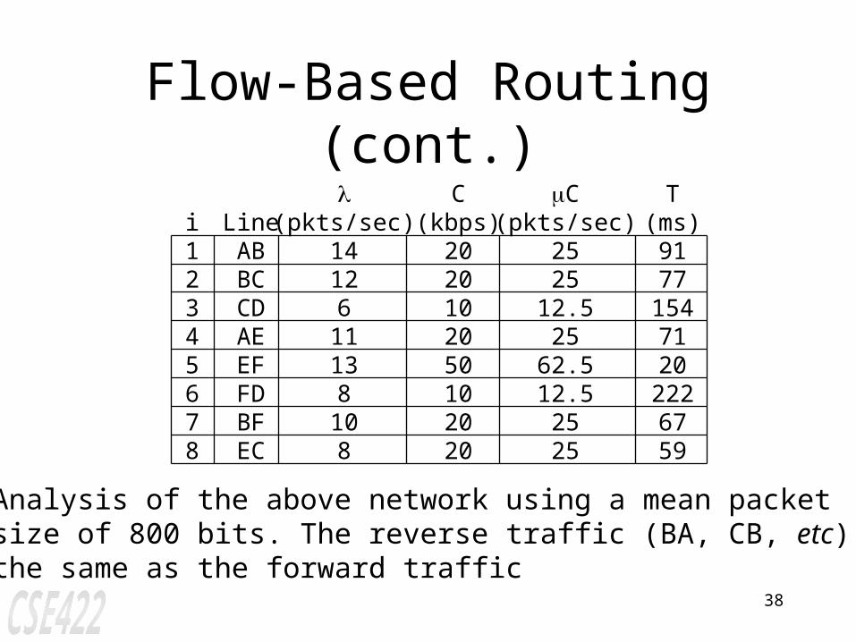
Flow-Based Routing (cont.)

i12345678

LineABBCCDAEEFFDBFEC

(pkts/sec)

14126

11138

108

C(kbps)

2020102050102020

C(pkts/sec)

2525

12.525

62.512.52525

T(ms)9177

1547120

2226759

Analysis of the above network using a mean packetsize of 800 bits. The reverse traffic (BA, CB, etc) isthe same as the forward traffic

39

Hierarchical Routing

1A - - 1B 1B 1 1C 1C 1 2A 1B 2 2B 1B 3 2C 1B 3 2D 1B 4 3A 1C 3 3B 1C 2 4A 1C 3 4B 1C 4 4C 1C 4 5A 1C 4 5B 1C 5 5C 1B 5 5D 1C 65E 1C 5

Dest. Line hops1A - - 1B 1B 11C 1C 1 2 1B 2 3 1C 2 4 1C 3 5 1C 4

Dest. Line hops

Full TableFor 1A

HierarchicalTableFor 1A

Region 1 Region 2

Region 3 Region 4 Region 5

1B

1A 1C

2A 2B

2D2C

5B5C

5D5E

5A4C4B

4A

3B

3A

40

Routing For Mobile Hosts

Foreign LAN

MAN

Home LAN

WAN

Homeagent

Wirelesscell

Mobilehost

A WAN to which LANs, MANs, and wireless cells are attached

41

Routing For Mobile Hosts (cont.)The registration procedure for mobile hosts:1. Periodically, each foreign agent broadcast a packet

announcing its existance and address. A newly arrived mobile host may wait for one of these messages, but if none arrives quickly enough, the mobile host can broadcast a packet saying: “Are there any foreign agents around?”

2. The mobile host registers with the foreign agent, giving its home address, current data link layer address, and some security information.

42

Routing For Mobile Hosts (cont.)3. The foreign agent contacts the mobile host’s home

agent and says: “One of your hosts is over here.” The message from the foreign agent to the home agent contains the foreign agent’s network address. It also includes the security information, to convince the home agent that the mobile host is really there.

4. The home agent examines the security information which contains a timestamp, to prove that it was generated within the past few seconds. If it is happy, it tells the foreign agent to proceed.

43

Routing For Mobile Hosts (cont.)5. When the foreign agent gets the acknowledgement

from the home agent, it makes an entry in its table and informs the mobile host that it is now registered.

44

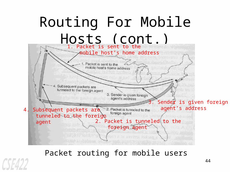
Routing For Mobile Hosts (cont.)

Packet routing for mobile users

1. Packet is sent to the mobile host’s home address

2. Packet is tunneled to the foreign agent

3. Sender is given foreign agent’s address4. Subsequent packets are

tunneled to the foreign agent

45

Broadcast Routing

46

Broadcast Routing (cont.)• Source to send a packet to each destination.

• Flooding.

• Multidestination routing -- each packet contains a list of destinations.

• Spanning tree -- copy an incoming packet onto all the spanning tree lines except the one it arrived on.

47

Traffic Control• Flow controle.g., Sliding window technique

• Congestion control e.g., Managing input and output buffers at IMPs.– Packets may be discarded or– A choke packet sent.

• Deadlocks e.g., No buffers are available.

48

Traffic Control (cont.)

To 1

To host

To 2

To 3

To 5Node 4

OutputBuffer

IntputBuffer

Input and OutputQueues at node 4

49

Traffic Control (cont.)

1

2 3

6

54

Host

The interaction of queues in a packet-switching network

50

The effects of congestion

(a) Throughput

throughput(packetsdelivered)

51

The effects of congestion (cont)

(b) Delay

AveragePacketDelay

52

Congestion Prevention Policies

Retransmission policy Out-of-order caching policy Acknowledgement policy Flow control policy Timeout determination Virtual circuits versus datagram inside the subnet Packet queueing and service policy Packet discard policy Routing Algorithm Packet lifetime management Retransmission policy Out-of-order caching policy Acknowledgement policy Flow control policy

Transport

Network

Data Link

Layer Policies

Policies that affect congestion

53

Traffic Shaping• Regulating the average rate (and burstiness) of data

transmission• monitoring a traffic flow is reffered as traffic

policing• Example: The leaky bucket algorithm used in

ATM networks (Turner 1986)• In contrast, sliding window protocols limit the

amount of data in transmission

54

Traffic Shaping (cont.)

HostComputer

A leaky bucket with water A leaky bucket with packet

Network

Packet

Unregulatedflow

The bucketholds

packets

Regulatedflow

Interfacecontaining

a leakybucket

55

Types of deadlock

(a) Direct store-and-forward deadlock

56

Types of deadlock (cont.)

(b) Indirect store- and- forward deadlock

57

Types of deadlock

(c) Reassembly deadlock

58

Structured buffer pool for deadlock avoidance.

Class N

Class K

Class 2Class 1

Command pool(Class 0)

Buffer space for packetsthat havetraveled k hops.