1 multitarget/multisensor tracking using only range and ... mmtusingrd.pdf · 1...

1

Multitarget/Multisensor Tracking using onlyRange and Doppler Measurements

Ross Deming,Member, IEEE,John Schindler,Life Fellow, IEEE,and Leonid Perlovsky,Senior Member, IEEE

Abstract

A new approach is described for combining range and Doppler data from multiple radar platformsto perform multi-target detection and tracking. In particular, azimuthal measurements are assumed tobe either coarse or unavailable, so that multiple sensors are required to triangulate target tracks usingrange and Doppler measurements only. Increasing the number of sensors can cause data association byconventional means to become impractical due to combinatorial complexity, i.e., an exponential increasein the number of target to signature mappings. When the azimuthal resolution is coarse, this problemwill be exacerbated by the resulting overlap between signatures from multiple targets and clutter. Inthe new approach the data association is performed probabilistically, using a variation of expectation-maximization. Combinatorial complexity is avoided by performing an efficient optimization in the spaceof all target tracks and mappings between tracks and data. The full, multi-sensor, version of the algorithmis tested on synthetic data. The results demonstrate that accurate tracks can be estimated by exploitingspatial diversity in the sensor locations. Also, as a proof-of-concept, a simplified, single-sensor, range-only, version of the algorithm is tested on experimental radar data acquired with a stretch radar receiver.These results are promising, and demonstrate a surprising degree of robustness in the presence ofnonhomogeneous clutter.

Index Terms

Multisensor systems, Optimization methods, Clustering methods, Distributed tracking, Radar tracking,Doppler radar, Radar data processing.

I. I NTRODUCTION

We present a new approach for multi-target detection and tracking, in which information frommultiple, spatially diverse, radar sensors is combined to improve track accuracy. In particular, we treatthe difficult case in which azimuthal measurements are either coarse or unavailable, so that multiplesensors are required to triangulate target tracks using range and Doppler measurements only. However,data association in this problem is extremely complex for several reasons. First, the coarse azimuthalresolution can result in significant overlap between the signatures of the multiple targets and clutter.Second, increasing the number of sensor platforms leads to an exponential increase in the number of

R. Deming and J. Schindler are consultants for General Dynamics Information Technology, Inc. L. Perlovsky is the technicaladvisor for the Air Force Research Laboratory, Sensors Directorate/SNHE. All work was conducted on-site at the Air ForceResearch Laboratory, Sensors Directorate/SNHE, 80 Scott Drive, Hanscom AFB, MA 01731, USA. Contact information forR.D.: [email protected], telephone: 781-377-1736.

February 7, 2007 DRAFT

2

mappings between actual targets and target signatures in the data. Thus, it becomes impractical to sortout the mappings using combinatorial approaches.

Multiple hypothesis tracking (MHT) [1], a benchmark optimal multi-target tracking algorithm, performsdata association using an exhaustive evaluation of all mappings between targets and data samples, and istherefore subject to a combinatorial explosion as the amount of data and the number of sensors increase.Typically, a pre-detect stage is used to alleviate the computational issue by reducing the number ofdata samples under consideration. Here, the low-amplitude or low-Doppler data samples below a certainthreshold are simply discarded. However, pre-detection leads to suboptimal performance and prevents thedetection of low signal-to-clutter (S/C) targets whose signatures lie below the threshold. An alternative toMHT is the joint probabilistic data association filter (JPDAF) [2], [3] which is more efficient than MHTbecause one only needs to evaluate the association probabilities separately at each time step. However,since all data association mappings are not considered, this method is not optimal [7], [8]. Also, JPDAF isgenerally not used for track initialization since detection is performed separately from tracking, whereasoptimum performance is only obtained when detection and tracking are performed concurrently [5], [16].Both MHT and JPDAF have been adapted for multi-sensor scenarios [3].

In the approach described here, data association is performed concurrently with detection and tracking,without a combinatorial explosion in computational requirements. Also, the approach is appropriate forhandling low S/C data and/or data with multiple, closely-spaced and overlapping targets. Whereas MHTand JPDAF are based upon “hard” associations between measurements and targets, i.e., selecting the bestdata-to-target mapping to calculate the track parameters, the method described here maps data to target andclutter components probabilistically. Here, the track parameters for a particular target are computed usinga weighted combination of all data samples, where the weights correspond to the association probabilities.An advantage of this framework is that it allows an efficient “hill climbing” optimization, to be performedin the space of all model parameters and all possible mappings between data samples and targets. In fact,this procedure can be framed as a special case of the expectation-maximization (EM) algorithm [9], [10],[11]. Like MHT, this algorithm is optimal [5], [6]. However, whereas the computational complexity ofMHT scales exponentially with the number of targets, data samples, and sensors, the method describedhere scales only linearly.

The general framework for the approach described in this paper was developed by Perlovsky in his workon multi-target tracking in clutter, automatic target recognition (ATR), and sensor fusion [5], [12], [13],[14], [15], [16], [17] (references contained in [6]). Perlovsky recognized, early on, that if classificationfeatures are available, an optimum algorithm will perform target classification concurrently with detectionand tracking, by mathematically placing the tracking coordinates (range, Doppler, bearing) on an equalfooting with classification features. Thus, the composite model of the data is expressed as a mixture oftarget and clutter components in the combined space of tracking and classification features. The algorithmdescribed here is based upon Perlovsky’s general approach [6] which we refer to asdynamic logic(DL).However, a major new aspect considered here is the data model, which is particularly complicated, andarises from combining data from multiple sensors, where azimuthal measurements are absent. Thus, thegoal here is to use multiple sensors to probabilistically triangulate target tracks using range and Dopplermeasurements only. An abbreviated version of this work was published previously [18], [19], althoughsome results and most of the mathematical details were not included.

Perlovsky’s DL tracker has much in common with a similar algorithm known as the probabilisticmultihypothesis tracker (PMHT) [7], [8], [20], [21] which was developed independently by Streit and


3

Luginbuhl, and shares strong similarities with Avitzour’s approach [22]. The major similarity betweenDL and these other trackers is the use of expectation-maximization (EM) [9], [10], [11] to perform dataassociation probabilistically, while simultaneously estimating track parameters. It should also be notedthat both PMHT [23], [24], [25] and DL [6], [26] have been adapted for combining data from multiplesensors. The chief difference between DL and PMHT is in the choice of track model. In PMHT themotion of each target is modeled using a set of discrete-time state transition equations, and therefore aKalman smoother is used to estimate track parameters in the M-step of the EM iterations [7], [20], [21]. Incontrast, DL is flexible with respect to the choice of track model, but it normally incorporates continuouspolynomial models (e.g., constant velocity, constant acceleration, etc.), or piecewise polynomial models,for target trajectories. The use of polynomial models leads to very simple parameter update formulas inthe M-step, for example, simple matrix inversions which are similar in structure to polynomial regression[6]. Of course, under certain conditions the discrete-time state transition equations used in PMHT wouldbe equivalent to the polynomial models used in DL. Another difference between PMHT and DL isthe choice of optimization criterion. Whereas in PMHT the goal is maximization of thea posterioriprobability [7] (MAP), in DL the goal is maximum likelihood estimation (MLE) in the case of sampleddata, and minimization of the cross-entropy in the case of pixelated data, which is the case in the presentapplication. Finally, as we stated above, the DL tracker is naturally structured for concurrent classificationand tracking when features are available.

When applied to a benchmark multi-target tracking problem, it was found that the computational cost ofPMHT has roughly the same order of magnitude as the cost of MHT and JPDAF [8]. Due to its structuralsimilarity to PMHT, the DL tracker would most likely have a similar computational cost when appliedto this problem. However, as mentioned above, the computational cost of the DL tracker scales onlylinearly with increasing numbers of sensors, whereas the cost of MHT scales exponentially. Therefore, itis expected that the cost advantages of the DL tracker – and therefore the cost advantages of the approachdescribed here – would become evident for the multi-sensor case.

The paper is organized as follows. In Sections II-IV the mathematical approach is developed forthe full, multi-sensor, version of the algorithm. The EM algorithm is a well established mathematicaltool for estimating the parameters in mixture models [9], [10], [11], and could certainly be used asa framework for deriving the solution to our problem, as was done for the PMHT [7], [20], [21].However, in this paper a different approach is offered, which Redner and Walker [11] refer to asthe “traditional general approach.” Here, a system of likelihood equations is derived, then solvedusing the partial derivatives of the optimization criterion. This basic procedure does not require anunderstanding of EM. In addition to the full, multi-sensor, algorithm, a simplified version is also derivedin Section V which is appropriate for performing range-only tracking from single-sensor data. In thiscase, the update formula for track parameters is particularly simple and efficient – it consists of asmall matrix inversion for each target component. Most of the mathematical details are contained inthe appendices. Appendix A contains a derivation of the parameter estimation equations for generalmixture models, and also tailors these equations to the tracking model used in this paper. Appendix Bcontains a convergence proof which, again, is within the structure of the traditional general approachrather than depending upon EM. Finally, in Section VI results are presented from experiments designedto test the algorithm. The simplified, range-only version is tested on experimental radar data, whilethe full, multi-sensor, version is tested on synthetic data. The results demonstrate a surprising degreeof robustness in the presence of nonhomogeneous clutter, and uncertainty in the number of targets present.


4

II. D ESCRIPTION OF THE SENSORS AND DATA.

The sensor model for this discussion incorporates a ground-based radar antenna whose dimensionsare on the same order as the transmitted wavelength. Such an antenna would have very poor azimuthalresolution and, in fact, we will assume the extreme case in which each sensor measures target rangeand Doppler (range-rate) only, but no azimuth. Thus, the 2-dimensional track of each target can only beestimated by triangulation from multiple, spatially diverse, sensor platforms.

Our method is appropriate for any collection of range/Doppler data, although as a working model itis assumed the data are acquired using a stretch receiver [27]. Here, a suite of long-duration chirps istransmitted from a stationary ground-based radar, and the corresponding suite of received signals withinthe coherent processing interval (CPI) is processed jointly to produce a two-dimensional digitized imagein range/Doppler coordinates, referred to as a “scan frame”. Examples of scan frames are shown inFigures 2 and 3 in Section VI, where the target signatures appear as blobs of energy centered uponthe true range and Doppler of the target. The brightness (strength) of each blob is proportional to therange and radar cross-section (RCS) of the corresponding target. The range resolution (i.e., the width ofthe blobs in the range coordinate) is a function of the bandwidth of the transmitted signals, while theDoppler resolution is a function of the CPI. Also, the Doppler resolution can be adversely affected bysensor platform vibration, and by nonlinear movement (i.e., acceleration) by the target.

In addition to the target signatures, range/Doppler images typically contain a strong signature fromstationary background clutter, which appears in the image as a ridge at zero Doppler across all rangebins (again, refer to Figures 2 and 3 in Section VI). The width of the ridge is is inversely proportionalto the CPI, and may also be affected by sensor platform vibration as well as the internal motion of theclutter (e.g., movement of leaves in the wind, etc.). Depending on its width, this clutter ridge may insome cases obscure or partially obscure the signatures from targets with small radial velocities. Finally,there will be a certain amount of background noise (receiver noise) which is uniformly distributed inrange/Doppler over the image.

It is assumed the data is collected as follows (Figure 1). At each time intervaltj , for j = 1, 2, 3, ..., J ,the received signals within the CPI centered attj are processed jointly to yield a digitized range/Dopplerimage (scan frame) as described above. Thus, for each sensorm = 1, 2, 3, ..., M we acquire a stackof J range/Doppler scan frames corresponding to the different time intervalstj . Note that, due to theirregular overlap in the fields of view of the different sensors, the signatures from some targets may notappear in the images from all sensors at all time intervals. Each range/Doppler scan frame image isdescribed using the notationp0(wjmn), wherep0 is the pixel intensity at the range/Doppler coordinatewjmn = (rjmn, djmn), which is indexed by time intervalj (i.e., scan frame numberj), sensorm, andpixel n = 1, 2, 3, ..., N . The total number of pixels in each scan frame isN = Nr ×Nd, whereNr andNd are the number of bins in range and Doppler, respectively. The width of each pixel with respectto range and Doppler is∆r and ∆d, respectively. The data from the multiple sensor platforms arecombined noncoherently to estimate target tracks, as described in the following sections.

III. M ODEL FOR THE DATA

A model for the datap0(wjmn) can be developed which depends upon the target trajectories as wellas the sensor parameters and coordinates. Suppose the coordinates of targetk at timetj are given by the


5

−8−6

−4−2

02

40

200400

600800

10001200

1

2

3

rangeDoppler

time

(sc

an fr

ame)

Fig. 1. Sample stack of three pixelated scan frames acquired with a particular sensor. The target signature appears as a highintensity (dark) blob centered around its true range/Doppler coordinate. Since the target is in motion, the signature position isslightly different in each scan frame. Similar data stacks would be acquired using other sensors, and the entire set of stacksfrom all sensors is processed jointly to estimate target tracks.

(east, north) coordinate(xk(tj), yk(tj)) ≡ (xjk, yjk). Using a constant acceleration model, the trajectoriesare described by

xjk = x0k + x′ktj + x′′kt

2j (1)

yjk = y0k + y′ktj + y′′kt2j . (2)

Here (x0k, y

0k) is the time-zero position of targetk, while (x′k, y

′k) is the time-zero velocity and(x′′k, y

′′k)

is the acceleration. To simplify the discussion, the targets are assumed to lie at zero elevation. Next,suppose there areM sensor platforms, where sensorm is fixed at the (east, north, elevation) coordinate(xm, ym, zm). Then, the rangeRkm(tj) ≡ Rjkm from sensorm to targetk at time tj is given by theequation

Rjkm =√

(xm − xjk)2 + (ym − yjk)2 + z2m. (3)

The Doppler (range-rate)Dkm(tj) = [∂Rkm(t)/∂t]t=tjis then

Dkm(tj) ≡ Djkm = −(

xm − xjk

Rjkm

)(x′k + 2x′′ktj)−

(ym − yjk

Rjkm

)(y′k + 2y′′ktj). (4)

As described in Section II, the target signatures appear as blobs of energy in the scan frame imagesp0(wjmn) approximately centered at the true range and Doppler coordinateswjmn = (Rjkm, Djkm). Wewish to construct a mathematical model that approximates these signatures, and for targetk we denotethis model aspk(wjmn|Θk), whereΘk is the set of model parameters. In this case it makes sense touse Gaussian distributions to model the target signatures (blobs of energy), so that the signature due to


6

targetk for sensorm and timetj is given by

pk(wjmn|Θk) =∆r∆d

2πσrkσdkexp

{−1

2

[(rjnm −Rjkm

σrk

)2

+(

djnm −Djkm

σdk

)2]}

. (5)

Here, the set of model parameters isΘk = {σ2dk, σ

2rk, x

0k, y

0k, x

′k, y

′k, x

′′k, y

′′k} where, in Eq.(5), the

track parameters{x0k, y

0k, x

′k, y

′k, x

′′k, y

′′k} are contained implicitly within the quantitiesRjkm and Djkm

according to Eqs. (3) and (4). Also,∆r and∆d define the pixel size relative to the range and Dopplercoordinates, as discussed in Section II. Note that the distribution in Eq.(5) is normalized1 so that∑N

n=1 pk(wjmn|Θk) = 1. The variance parameterσ2rk specifies the width of the signatures with respect

to the range coordinate in the scan frame image, and is related to the range resolution of the sensor. Theother variance parameterσ2

dk specifies the the width of the signature in Doppler, and depends both onthe sensor resolution and the target motion, including internal (micro) motion.

The clutter also requires a model, and we will approximate this clutter using two components, one forthe uniform background noise (receiver noise), and one for the stationary clutter. We will designate thetwo clutter indices ask = (K − 1),K and the target indices ask = 1, 2, 3, ..., (K − 2). The backgroundnoise (receiver noise) componentk = K − 1, uniform in both range and Doppler, is described by

pK−1(wjmn|ΘK−1) =1N

, (6)

whereN is the number of pixels in each range/Doppler image, as discussed above. The1/N factor isnecessary for normalization, i.e., to insure

∑Nn=1 pk(wjmn|Θk) = 1. Note, here the set of parameters

ΘK−1 is empty. The second clutter componentk = K, which models the reflected energy from stationaryground clutter, is uniform in range, and zero-mean Gaussian in Doppler, i.e.,

pK(wjmn|ΘK) =∆d√

2πσdkNr

exp

{−1

2

(djnm

σdK

)2}

. (7)

Here,Nr is the number of range bins in each pixel array, as discussed in the previous section. Note, herethe set of parameters isΘK = {σ2

dK}. A further discussion of clutter modeling is given in [6].

The total model for the image data is the weighted summation (mixture) of individual target and cluttercomponents

p(wjmn|Θ) =K∑

k=1

Ekm pk(wjmn|Θk). (8)

Here,Ekm is the relative weighting for each of the model components, which we refer to as themixtureweight. For target components, the mixture weight is proportional to the target’s radar cross-section (RCS)and range as viewed by sensorm. Since RCS can be strongly dependent upon aspect angle, we allowEkm to depend upon both targetk and sensorm. Also, this dependence upon sensorm allows for the factthat the fields-of-view for the different sensors overlap in an irregular manner, so that a signature froma certain target may not appear in the data from all sensors. In Eq.(8), the total set of model parametersis denoted byΘ = {Ekm,Θk}, wherek = 1, 2, ..., K andm = 1, 2, ..., M .

1Actually, the normalization is approximate, and assumes the pixel dimensions(∆r, ∆d) are small relative to(σrk, σdk).


7

By summing both sides of Eq.(8) over the pixel indexn, and using the (previously stated) fact that∑Nn=1 pk(wjmn|Θk) = 1, we obtain

∑n

p(wjmn|Θ) =∑

k

Ekm. (9)

It is sensible to place a constraint so that, for each scan framej and sensorm, the total energy in themodel equals the total energy in the measured data, i.e.,

∑n p(wjmn|Θ) =

∑n p0(wjmn). Combining

this constraint with Eq.(9), we obtain the following constraint on the mixture weight parameters, validfor every scan framej and sensorm:

∑n

p(wjmn|Θ) =∑n

p0(wjmn) =∑

k

Ekm. (10)

IV. PARAMETER ESTIMATION

The goal is to find the set of model parametersΘ = {Ekm,Θk} providing the best match between thethe modelp(wjmn|Θ) and the datap0(wjmn). The model, described in Section III, is completely specifiedby the the mixture weightsEkm, the variancesσ2

dk andσ2rk, and the parameters{x0

k, y0k, x

′k, y

′k, x

′′k, y

′′k}

describing the target trajectories. In this paper theEinsteinian log-likelihood([6], chapter 4.4.1)

LL(Θ) =∑

j,m,n

p0(wjmn) ln p(wjmn|Θ) =∑

j,m,n

p0(wjmn) lnK∑

k=1

Ekmpk(wjmn|Θk) (11)

will serve as a criterion to quantify the similarity between the model and the data. Given the constraintin Eq.(10), it can be shown thatLL will be maximized when the model and the data match, i.e., forp(wjmn|Θ) = p0(wjmn). Note that maximizingLL is equivalent to minimizing the cross-entropy, a.k.a,the Kullback-Liebler (KL) divergence, a well-established metric from the information theory arena [32].Mathematical and physical justifications for both Einsteinian log-likelihood and the KL divergence havebeen discussed in detail [6], [28], [29], [30], [31].

The mathematical details of the optimization are contained in Appendix A. Briefly, by a system ofequations is derived which is satisfied by the parameters maximizingLL, subject to the constraint ofEq.(10). Unfortunately, an analytical solution is intractable since the system of equations is a large,coupled, set of nonlinear equations. However, various iterative techniques can be employed for solvingthe set of likelihood equations and, in Appendix A, an efficient technique is described which is actually aspecial case of EM. This technique defines a recursive update formula for each parameter. For example,using the notationE(I)

km and Θ(I)k to indicate the estimates of the parameters at theIth iteration, the

recursive update formulas forEkm, σ2dk, andσ2

rk are given by

E(I+1)km =

1J

∑

j,n

p0(wjmn)P (I)(k|jmn), (12)

(σ2

dk

)(I+1)=

∑j,m,n p0(wjmn)P (I)(k|jmn) (djnm −Djkm)2

∑j,m,n p0(wjmn)P (I)(k|jmn)

, (13)


8

and

(σ2

rk

)(I+1)=

∑j,m,n p0(wjmn)P (I)(k|jmn) (rjnm −Rjkm)2

∑j,m,n p0(wjmn)P (I)(k|jmn)

, (14)

where

P (I)(k|jmn) =E

(I)km pk(wjmn|Θ(I)

k )∑

k′ E(I)k′mpk′(wjmn|Θ(I)

k′ )=

E(I)km pk(wjmn|Θ(I)

k )p(wjmn|Θ(I))

. (15)

There is an analogous rule for updating the tracking parameters{x0k, y

0k, x

′k, y

′k, x

′′k, y

′′k}, which is described

later in this section. The equations above imply that one start with an initial guess for the parameters{E(0)

km, Θ(0)k }, then alternate between updatingP (I)(k|jmn) using Eq.(15), then updating the parameters

{E(I+1)km ,Θ(I+1)

k } using Eqs. (12)-(14). In fact, these steps correspond to the E-step and the M-step,respectively, of the EM algorithm. This iterative procedure is guaranteed to converge to a local maximumof LL, as shown in Appendix B. Note that the mixture weightsEkm are updated using Eq.(12) for alltarget and clutter componentsk = 1, 2, ..., K. In fact, Eq.(12) is appropriate for updating the weights ofarbitrary mixture models, not only the tracking model considered here. The variancesσ2

dk and σ2rk are

updated for the appropriate model components, as indicated by the target and clutter model equations.Since the variance parameters are initialized to large values, the components are initially fuzzy andindistinct. However, with increasing iterations, the variances tend to adapt by shrinking, and the individualcomponents will gradually lock on to the target signatures, or to portions of the clutter. Thus, the modeliteratively adapts to fit the data, as we demonstrate with the results in Section VI.

If the model is viewed probabilistically ([6], chapter 4.4.8), then Eq.(15) is simply a form of Bayes’rule, and the quantitiesP (I)(k|jmn) can be construed as the probabilities that the energy in pixel(j,m, n)originates from target or clutter componentk. Therefore,P (I)(k|jmn) are referred to as the “associationprobabilities”. Eq.(12) therefore makes intuitive sense – it simply states thatE

(I+1)km is the sum of all

pixel valuesp0(wjmn), where the pixels are weighted by their association probabilities. Similarly, Eqs.(13) and (14) correspond to the usual definition of sample covariance, however with pixels weighted bytheir association probabilities. From Eq.(15) it is easy to see that

∑

k

P (I)(k|jmn) = 1 (16)

for any iterationI.It will be convenient to define the angled bracket notation

〈∗〉(I) ≡∑

j,n

p0(wjmn)P (I)(k|jmn)(∗), (17)

where the asterisk∗ denotes a generic quantity. Thus, Eqs. (12) - (14) can be rewritten in the compactform

E(I+1)km =

〈1〉(I)

J, (18)

(σ2

dk

)(I+1)=

∑m〈(djnm −Djkm)2〉(I)

∑m〈1〉(I)

, (19)

and (σ2

rk

)(I+1)=

∑m〈(rjnm −Rjkm)2〉(I)

∑m〈1〉(I)

. (20)


9

Whereas the Doppler varianceσ2dk of target signatures are related to the target dynamics, the range

varianceσ2rk is related only to the sensor resolution, which is knowna priori. Therefore, rather than

adaptively estimating this parameter using Eq.(20), it may be advantageous to evolveσrk according to apredetermined schedule [6], [15], [16], [17]. For example,σrk can be initialized to a rather large value,so that the target components can “see” large sections of the pixel data, then shrunk according to anexponential decay over iterations to a steady state value corresponding to the sensor resolution.

Finally, the recursive update formula is derived for the tracking parameters{x0k, y

0k, x

′k, y

′k, x

′′k, y

′′k},

k = 1, 2, 3, ..., (K − 2). In the single-sensor case, described below in Section V, the update formulafor these parameters is a simple closed-form expression, analogous to Eqs. (18) - (20). Unfortunately, aclosed-form update formula cannot be derived for the general multi-sensor case. However, convergencewill still be guaranteed (see Appendix B) if the tracking parameters are simply “nudged” along theuphill gradient ofLL during each iteration. This actually corresponds to a special case of the generalizedEM (GEM) procedure [10]. Usingsk as a generic placeholder for any one of the tracking parameters{x0

k, y0k, x

′k, y

′k, x

′′k, y

′′k}, the update formula is given by

s(I+1)k = s

(I)k + h ·

[∂LL

∂sk

], (21)

whereh is the gradient ascent stepsize, and

∂LL

∂sk=

∑m

⟨(rjnm −Rjkm

σ2rk

) (∂Rjkm

∂sk

)⟩(I)

+∑m

⟨(djnm −Djkm

σ2dk

) (∂Djkm

∂sk

)⟩(I)

. (22)

This expression is derived in Appendix A. It is straightforward to compute explicit expressions for∂Rjkm/∂sk and ∂Djkm/∂sk for each of the parameterssk = {x0

k, y0k, x

′k, y

′k, x

′′k, y

′′k} using Eqs. (3)

and (4). For example,∂Rjkm/∂x0k = − (xm − xjk) /Rjkm. Although Eq.(21) describes a single gradient

ascent step during each iteration, multiple steps can be taken during each iteration while holding theassociation probabilitiesP (k|jmn) fixed. In practice, the convergence rate can be optimized, using trial-and-error to determine a suitable combination of stepsizeh and steps/iteration.

Although the present study is mainly concerned with tracking, it is important to consider the issue ofautomatic detection and target declaration. The standard detection approach, e.g., described in reference[6], section 7.2.9, utilizes a log-likelihood ratio test which operates on the converged parameter values.The issue of detection will be studied in more detail in a future publication.

V. RANGE-ONLY TRACKING FROM A SINGLE SENSOR.

If only a single sensor platform is available, and measurements of azimuth are unavailable, it maystill be desirable to perform range-only tracking. Here, the target and clutter models given by Eqs.(5)-(7)are still valid, as well as the total model for the data given by Eq.(8). Also, the variance(σ2

dk, σ2rk) and

mixture weightEkm parameters are still updated using Eqs. (18)-(20). However, in the single-sensorcase the target track parameters can be updated using a closed-form formula, which is simpler and moreefficient than the gradient ascent procedure described by Eq.(21) used for the multi-sensor case. Note thatthe analysis in this section is very similar to the analysis given in [6], chapter 7.2.6. However, whereasan update formula was given for a constant velocity model in the previous work, constant accelerationtrack models are used here.


10

Suppose the range between the targets and the (single) sensor can be described using a constantacceleration model, i.e.,

Rjkm = R0k + R′

ktj + R′′kt

2j , (23)

where R0k is the time-zero range of targetk, R′

k is the time-zero range-rate andR′′k is the range-

acceleration. Although there is only a single sensorm = 1, them subscript is maintained in the quantityRjkm for consistency with the expression for the target model in Eq.(5). The Doppler (range-rate) at timetj is the derivative of range with respect to time evaluated attj , or

Djkm = R′k + 2R′′

ktj . (24)

In Appendix A, an update formula is derived for iteratively adjusting the values of{R0k, R

′k, R

′′k} in

order to maximizeLL which, as in the multi-sensor case, is described by Eq.(11). This update formula isdescribed by a3×3 set of linear equations, which can be expressed using the following matrix notation:

H̄

(R0

k

)(I+1)

(R′k)

(I+1)

(R′′k)

(I+1)

=

〈rjnm〉 /σ2rk

〈rjnmtj〉 /σ2rk + 〈djnm〉 /σ2

dk

⟨rjnmt2j

⟩/σ2

rk + 〈2djnmtj〉 /σ2dk

(25)

where

H̄ =1

σ2rk

〈1〉〈tj〉⟨t2j

⟩

〈tj〉⟨t2j

⟩ ⟨t3j

⟩

⟨t2j

⟩ ⟨t3j

⟩ ⟨t4j

⟩

+1

σ2dk

0 0 0

0 〈1〉〈2tj〉

0 〈2tj〉⟨4t2j

⟩

.

Here, for example,(R0

k

)(I+1) denotes the updated estimate forR0k computed at the(I + 1)th iteration.

For the sake of compactness, the(I) superscript has been omitted from the angled bracket notation〈∗〉used for the elements in the above matrices. However it should be understood that

〈∗〉 ≡∑

j,n

p0(wjmn)P (I)(k|jmn)(∗). (26)

It can be shown that, in the absence of Doppler measurements, this set of equations (25) is equivalent tosecond order polynomial regression in which data samples are weighted by their association probabilities.

Unlike the update formulas forEkm, σdk, and σrk, given by Eqs. (18)-(20), the matrix expression(25) actually represents a set of three coupled update formulas for the three tracking parameters{R0

k, R′k, R

′′k}. Upon each iteration, these parameters are updated by inverting Eq.(25). Note that a

separate3× 3 matrix inversion is performed for each target componentk = 1, 2, ..., (K − 2).


11

VI. RESULTS

Results are now presented from computational experiments designed to test the algorithm. In the firsthalf of this section the simplified, single-sensor, range-only, version of the algorithm is tested usingexperimental stretch radar data [27] received from Lincoln Laboratory and DARPA. In the second half,results are presented using the full, multi-sensor, version of the algorithm. Since experimental multi-sensordata was not available, multi-sensor results are based upon synthetic data.

Let us now describe the single-sensor results computed from experimental data, using the simplifiedversion of the algorithm described in Section V. These results will be mainly qualitative since true targettracks were not provided, nor detailed information about the radar. Nevertheless, this analysis will serveas a useful proof-of-concept for the algorithm. The experimental setup consisted of a stretch receivermounted on a tower overlooking a wooded area, and data was collected as various targets moved throughthe area. The raw data was converted to a suite of range/Doppler scan frames using standard processingtechniques [27], as discussed in Section II. The algorithm described in Section V was used to jointlyprocess multiple sets of scan frames, where each scan frame is computed from data centered around adifferent timetj , j = 1, 2, ..., J .

Data, time = 0 seconds

Doppler (m/sec)

rang

e (m

)

−20 −10 0 10 20

140

160

180

200

220

240

260

280

Model, iteration= 5

Doppler (m/sec)

rang

e (m

)

−20 −10 0 10 20

140

160

180

200

220

240

260

280

Model, iteration= 30

Doppler (m/sec)

rang

e (m

)

−20 −10 0 10 20

140

160

180

200

220

240

260

280


Doppler (m/sec)

rang

e (m

)

−20 −10 0 10 20

140

160

180

200

220

240

260

280

1.5

2

2.5

3

3.5

Fig. 2. Upper left: scan frame data acquired at timet = 0 seconds in which a single target signature appears at Dopplerand range values of roughly (-12 m/sec) and (258 m), respectively. The remaining three plots show the evolution of the model,which adapts to fit the data as iterations increase. The white X’s in the lower right plot indicate the converged range/DopplercoordinatesR0

k andR′k for the target components in the model.

The upper left plot of Figure 2 shows a single scan frame acquired at a reference time oft = 0 seconds.A target signature appears as a “blob of energy” at Doppler and range values of roughly (-12 m/sec)and (258 m), respectively. There is a significant ridge of clutter from the stationary background centered


12


Doppler (m/sec)

rang

e (m

)

−20 −10 0 10 20

140

160

180

200

220

240

260

280

Model, iteration= 5

Doppler (m/sec)

rang

e (m

)

−20 −10 0 10 20

140

160

180

200

220

240

260

280


Doppler (m/sec)

rang

e (m

)

−20 −10 0 10 20

140

160

180

200

220

240

260

280


Doppler (m/sec)ra

nge

(m)

−20 −10 0 10 20

140

160

180

200

220

240

260

280

1.5

2

2.5

3

3.5

Fig. 3. Same as Figure 2, however here the scan frame was acquired at a later time oft = 6 seconds. The target signaturehas now moved to Doppler and range values of roughly (-9 m/sec) and (195 m), respectively.

at zero Doppler, extending across all range bins. There is also a clutter background which is roughlyuniform in range/Doppler, although with some significant inhomogeneities. For the model we used fivecomponents; three target components plus one uniform background clutter component, plus one cluttercomponent shaped like a ridge centered at zero Doppler.

The remaining three plots of Figure 2 show how the model evolves with increasing iterations. Sincethe model variances are initialized to large values, the model is initially broad, fuzzy, and indistinct(upper right). However, as the iterations progress, the parameters adapt in such a way to eventuallydefine a model which shares most of the significant features of the data. The lower right plot in Figure 2shows the converged model after 200 iterations. Here the white X’s indicate the converged range/DopplerestimatesR0

k andR′k for the three target components. Notice that one of the three target components has

nicely locked on to the true target signature, while the extra two target components have been useful formodeling the inhomogeneous regions of the background clutter. Although Figure 2 shows the data andmodel corresponding to only a single scan frame, it is important to note that the results were computedby jointly processing10 scan frames, starting att = 0 and proceeding in intervals of0.25 seconds.

The upper left plot of Figure 3 shows a scan frame data corresponding to a different time,t = 6seconds. The target signature has now moved to Doppler and range values of roughly (-9 m/sec) and(195 m), respectively. Here, the inhomogeneities in the background are even more extreme than for thet = 0 case shown in Figure 2. However, the model was still able to adapt quite nicely, with one of thetarget components locking on to the true target signature, and the extra components adapting to fit theclutter.


13


Doppler (m/sec)

rang

e (m

)

−20 −10 0 10 20

140

160

180

200

220

240

260

280


Doppler (m/sec)

rang

e (m

)

−20 −10 0 10 20

140

160

180

200

220

240

260

280

1

2

3

4

5

6

7

8

Fig. 4. The left-hand plot shows the same scan frame shown in Figure 3, however a large amount of artificial noise was addedwhich almost completely obscures the target signature. Nevertheless (right-hand plot), one of the model components was ableto adapt to a range/Doppler coordinate in the close vicinity of the target signature.

In Figures 2 and 3, the target signatures were rather strong, with signal-to-clutter ratios (S/C) of roughly3 dB. Next, the tracking experiment was repeated for the same case shown in Figure 3, however theproblem was intentionally made more difficult by adding a large amount of artificial noise, so that theS/C was reduced to roughly0 dB. This noise is uniformly distributed in range and Doppler, and issignal-independent, i.e., it was simply added to the intensity image. The data and the converged modelfor this noisy experiment are shown in Figure 4, which shows that the model was able to lock onto thetarget signature in the data, despite the fact that the target signature is almost completely obscured bythe added noise.

Although the present study is mainly concerned with tracking, it is important to consider the issue ofautomatic detection and target declaration. For example, in the converged model shown in the lower rightplot of Figure 3 there are three target components which converged to the three different range/Dopplercoordinates shown by the white X’s. One component has locked on to the target signature, while theother two have adapted to fit portions of the clutter. Here, the detection problem consists of automaticallydeclaring the true target, while disregarding the other two components. The standard detection approach,e.g., described in reference [6], section 7.2.9, utilizes a log-likelihood ratio test which operates on theconverged track and variance parameter values. In the examples shown thus far, it appears that perhapsa simple detection algorithm could be devised based upon the compactness of the target component, i.e.,based upon the converged values of the variance parametersσdk andσrk. The issue of detection will bestudied in more detail in a future publication.

Next, sample results are presented in which tracking was performed over longer time intervals. Here, asliding window approach was used to estimate tracks along extended, irregular, paths in the range/Dopplerspace. Overlapping sets of6 scan frames at a time were used to compute each point along the path. Forexample, the first point on the path was computed by jointly processing6 scan frames within the timeinterval 0 ≤ tj ≤ 1.25 seconds, the second point on the path was computed by jointly processing6 scanframes within the time interval0.5 ≤ tj ≤ 1.75 seconds, etc. Figure 5 shows results from tracking asmoothly decelerating target. Four different scan frames are shown corresponding to times oft = 0, 2.5, 6,

and12 seconds. Superimposed on the images is a dark line which indicates the extended track computedusing the sliding window method over a12 second interval. Notice the close agreement between thelocation of the target signatures and the computed track. Next, Figure 6 shows results from tracking a


14

Time = 0 seconds

Doppler (m/sec)

rang

e (m

)

−20 −15 −10 −5 0 5

140

160

180

200

220

240

260

280

Time = 12 seconds

Doppler (m/sec)ra

nge

(m)

−20 −15 −10 −5 0 5

140

160

180

200

220

240

260

280

Time = 6 seconds

Doppler (m/sec)

rang

e (m

)

−20 −15 −10 −5 0 5

140

160

180

200

220

240

260

280

Time = 2.5 seconds

Doppler (m/sec)

rang

e (m

)

−20 −15 −10 −5 0 5

140

160

180

200

220

240

260

280

Fig. 5. Tracking over extended time interval for smoothly decelerating target. Each scan frame corresponds to a different timeinstance with a 12 second interval. Overlaid is a dark line showing the track computed using our method.

time = 0 seconds

Dopper (m/sec)

rang

e (m

)

−20 −10 0 10 20

500

550

600

650

700

2

2.5

3

3.5

4

time = 7.5 seconds

Dopper (m/sec)

rang

e (m

)

−20 −10 0 10 20

500

550

600

650

700

2

2.5

3

3.5

4

time = 11 seconds

Dopper (m/sec)

rang

e (m

)

−20 −10 0 10 20

500

550

600

650

700

2

2.5

3

3.5

4

time = 15.5 seconds

Dopper (m/sec)

rang

e (m

)

−20 −10 0 10 20

500

550

600

650

700

2

2.5

3

3.5

4

Fig. 6. Tracking over extended time interval for maneuvering target. Each scan frame corresponds to a different time instancewithin a 15.5 second interval. Overlaid is a dark line showing the track computed using our method.


15

maneuvering target. Here the target accelerates significantly over the time observation interval, whereaspreviously the target velocity changed relatively slowly. Each scan frame in Figure 6 corresponds to adifferent time instance within a 15.5 second interval. Overlaid is a dark line showing the track computedusing the sliding window method which, again, shows close agreement between the location of the targetsignatures and the computed track.

−50 0 50 100 150

0

20

40

60

80

100

120

140

160

x = east position (m)

y =

nor

th p

ositi

on (

m)

1 2 3 4

5

sensorstargets

Fig. 7. Geometry for the multi-sensor simulation.

In the remainder of this section results are presented from the full, multi-sensor, version of the algorithmdescribed in Section IV. Since experimental multi-monostatic data was unavailable to us, the results arebased upon sets of synthetic range/Doppler scan frames, e.g., of the type that would be produced fromUHF stretch radar data [27]. In these simulations, the emphasis was more on data association thandetection performance, therefore the data was generated with a relatively high signal-to-clutter ratio(S/C), roughly8 dB. However, the zero-Doppler ridge from stationary clutter was generated with highenough amplitude to overlap and obscure the low-Doppler target signatures (Figure 8). In these cases,the S/C was more like0− 3 dB.

Figure 7 shows the geometry for the experiment. There are5 sensors and4 targets, two of which haveconstant velocity and two of which are accelerating. Sensors1− 3 are spaced roughly10 meters apart2,while the positions of sensors4 and5 are more widely spaced so that the spatial diversity can be usedto “triangulate” accurate track estimates for the targets. The targets were observed by all five sensors at4 different time intervals separated by0.25 seconds. Thus, the algorithm was required to jointly processa total of twenty scan frames in order to estimate target tracks. Figure 8 shows four of these twenty scanframes, corresponding to sensors1 and5 at timest1 = 0 and t4 = 0.75 seconds. From this figure it isapparent that the data association problem is non-trivial. For example, it is not obvious “by eye” whichsignatures in the bottom-right plot of Figure 8 correspond to which signatures in the top-left plot.

2Sensors1− 3 do not operate as an array since their data is processed noncoherently.


16

Doppler (m/sec)

rang

e (m

)

time = 0, sensor = 1

−15 −10 −5 0 5 10 15

50

100

150

200

2

4

6

8

10

12

14

16

time = 0.75, sensor = 1

Doppler (m/sec)

rang

e (m

)

−15 −10 −5 0 5 10 15

50

100

150

200

time = 0, sensor = 5

Doppler (m/sec)

rang

e (m

)

−15 −10 −5 0 5 10 15

50

100

150

200time = 0.75, sensor = 5

Doppler (m/sec)

rang

e (m

)−15 −10 −5 0 5 10 15

50

100

150

200

Fig. 8. Synthetic range/Doppler image data showing the scan frames for sensor1 (time= 0, 0.75 seconds) and sensor5(time= 0, 0.75 seconds). There are4 target signatures present. Note that the signatures of the lower-velocity targets significantlyoverlap the clutter ridge centered at zero Doppler.

Doppler (m/sec)

rang

e (m

)

iteration = 9

−15 −10 −5 0 5 10 15

50

100

150

200iteration = 16

Doppler (m/sec)

rang

e (m

)

−15 −10 −5 0 5 10 15

50

100

150

200

iteration = 23

Doppler (m/sec)

rang

e (m

)

−15 −10 −5 0 5 10 15

50

100

150

200iteration = 30

Doppler (m/sec)

rang

e (m

)

−15 −10 −5 0 5 10 15

50

100

150

200

2

4

6

8

10

12

14

16

Fig. 9. Model evolution for the sensor1, time= 0 data. Compare the converged model (bottom-right plot here) to the theactual data (top-left plot of Figure 8).


17

20 40 60 80 100

−15

−10

−5

0

5

10

iteration

xk’ = time−zero velocity, east (m/s)

c1c2c3c4c5c6truth

20 40 60 80 10040

50

60

70

80

90

100

110

120

xk0 = time−zero position, east (m)

iteration

20 40 60 80 100−2.5

−2

−1.5

−1

−0.5

0

0.5

1

xk’’ = acceleration, east (m/s 2)

iteration20 40 60 80 100

0

50

100

150

mixture weight Ek

iteration

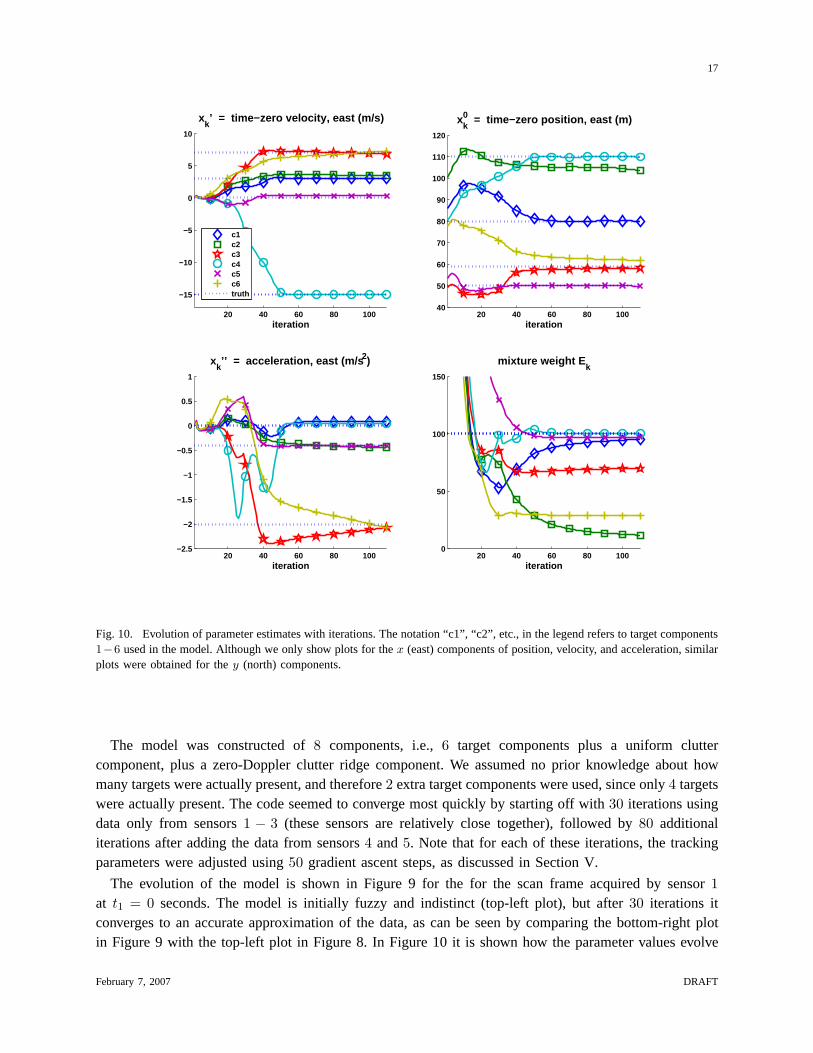
Fig. 10. Evolution of parameter estimates with iterations. The notation “c1”, “c2”, etc., in the legend refers to target components1−6 used in the model. Although we only show plots for thex (east) components of position, velocity, and acceleration, similarplots were obtained for they (north) components.

The model was constructed of8 components, i.e.,6 target components plus a uniform cluttercomponent, plus a zero-Doppler clutter ridge component. We assumed no prior knowledge about howmany targets were actually present, and therefore2 extra target components were used, since only4 targetswere actually present. The code seemed to converge most quickly by starting off with30 iterations usingdata only from sensors1 − 3 (these sensors are relatively close together), followed by80 additionaliterations after adding the data from sensors4 and5. Note that for each of these iterations, the trackingparameters were adjusted using50 gradient ascent steps, as discussed in Section V.

The evolution of the model is shown in Figure 9 for the for the scan frame acquired by sensor1at t1 = 0 seconds. The model is initially fuzzy and indistinct (top-left plot), but after30 iterations itconverges to an accurate approximation of the data, as can be seen by comparing the bottom-right plotin Figure 9 with the top-left plot in Figure 8. In Figure 10 it is shown how the parameter values evolve


18

during the adaptation of the model. Separate plots are given for the east (x) components of time-zerovelocity x′k, time-zero positionx0

k, and accelerationx′′k. Similar plots were obtained for they (north)componentsy′k, y0

k, andy′′k , but they are not shown here. In Figure 10, a plot is also given showing theevolution of the mixture weightsEk for each of the target components (Ek of clutter components arenot shown).

As mentioned above, the first30 iterations were performed using data only from sensors1− 3 whilethe remaining iterations were performed using all data from sensors1− 5. There are curves in the plotsof Figure 10 for each of the6 target components labelled “c1-c6” , and these are compared with thetrue parameter values (dashed lines). Recall, there are only4 targets actually present. From the plots, itcan be seen that components c1, c4, and c5, converge asymptotically to the true target parameters. Incontrast, component c2 seems to drift around without locking onto a target, and its corresponding mixtureweight parameter decreases toward zero with increasing iterations. Based upon its dwindlingEk value,component c2 could easily be pruned from the model. The most interesting case involves componentsc3 and c6, which seem to lock onto the same target, as shown by the fact that their velocity, position,and acceleration estimates converge together in order to share a true target track. The mixture weightparameterEk plot (right-most plot) shows that the weights for c3 and c6 roughly sum up to the truemixture weight of100. Presumably, it would be straightforward to detect this condition in which twocomponents lock onto the same target. Then one of the two could simply be pruned from the model ifnecessary.

VII. C ONCLUSIONS

In this paper we describe a mathematical algorithm for robust multi-target tracking from multipleradar platforms, for difficult cases in which measurements of azimuth are unavailable. A simplifiedversion of the algorithm is also presented which is appropriate for range-only tracking from a singleradar platform. Results are presented from computational experiments designed to test the algorithm. Thesingle-sensor, range-only, algorithm is tested on experimental data. These results show the approach to bevery promising, and robust in the presence of significant, inhomogeneous, background clutter. The full,multi-sensor, algorithm is tested on synthetic data. These results demonstrate that accurate tracks can beestimated by exploiting spatial diversity in the sensor locations. Furthermore, the algorithm appears tobe robust in the presence of significant clutter, and uncertain knowledge regarding the number of targetspresent.

ACKNOWLEDGMENT

This research was supported by Dr. John Sjogren of the Air Force Office of Scientific Research. Theauthors would like to thank scientists from DARPA and Lincoln Laboratory for supplying radar data andtechnical assistance.


19

APPENDIX A. DERIVATION OF PARAMETER ESTIMATION EQUATIONS.

Here the equations are derived which are satisfied by the parameters maximizingLL subject to aconstraint. The general procedure is first developed, valid for an arbitrary mixture model. These resultsare then used to derive the particular equations corresponding to the tracking model.

First, consider maximizingLL using a general mixture model. One might seek to maximizeLL

directly, by finding values for the set of parametersΘk for which all partial derivatives∂LL/∂Θk arezero. Using the expression forLL from Eq.(11),

∂LL

∂Θk=

∑

j,m,n

p0(wjmn)∂

∂Θk

[ln

∑

k′Ek′m pk′(wjmn|Θk′)

]

=∑

j,m,n

[p0(wjmn)∑

k′ Ek′mpk′(wjmn|Θk′)

]∂

∂Θk[Ekm pk(wjmn|Θk)]

=∑

j,m,n

p0(wjmn)

[Ekm pk(wjmn|Θk)∑k′ Ek′mpk′(wjmn|Θk′)

]∂

∂Θk[Ekm pk(wjmn|Θk)]

Ekm pk(wjmn|Θk)

=∑

j,m,n

p0(wjmn)P (k|jmn)∂

∂Θkln [Ekm pk(wjmn|Θk)] . (27)

Here, we made use of the well-known identity∂ ln y(x)∂x = [1/y(x)]∂y(x)

∂x , and the definition of

P (k|jmn) =Ekm pk(wjmn|Θk)∑k′ Ek′mpk′(wjmn|Θk′)

. (28)

Using Eq.(27), the set of parametersΘk that maximizeLL will satisfy

∂LL

∂Θk=

∑

j,m,n


∂Θkln pk(wjmn|Θk) = 0, (29)

The maximization ofLL must also be performed with respect to the mixture weightsEkm, howeverit is now necessary to incorporate the constraint from Eq.(10) using the method of Lagrange multipliers.Thus we seek to minimize the Lagrangian

F = −LL + λ

(∑

k′Ek′m −

∑n

p0(wjmn)

)(30)

with respect toEkm, whereλ is the Lagrange multiplier. Setting the partial derivative ofF to zero, i.e.,

∂F

∂Ekm= − ∂LL

∂Ekm+ λ = 0, (31)

the following value forλ is obtained:

λ =∂LL

∂Ekm. (32)

An expression for∂LL/∂Ekm is now needed, and its derivation is similar to Eq.(27). We obtain

∂LL

∂Ekm=

∑

j,n


∂Ekmln [Ekm pk(wjmn|Θk)] =

1Ekm

∑

j,n

p0(wjmn)P (k|jmn).


20

Combining this with Eq.(32),

λEkm =J∑

j=1

N∑

n=1

p0(wjmn)P (k|jmn). (33)

Next we perform the summation overk on both sides of Eq.(33), then use Eqs. (10) and (16) to simplify.This results in the solution for the Lagrange multiplierλ = J , whereJ is the number of scan frames(time intervals) from each sensor used in the estimation. Substituting this value back into Eq.(33), weobtain

Ekm =1J

∑

j,n

p0(wjmn)P (k|jmn). (34)

Eq.(34) is satisfied by the set of mixture weightsEkm that maximizeLL, subject to the constraint inEq.(10).

A set of equations has now been derived governing the complete set model parametersΘ = {Ekm, Θk},for k = 1, 2, ..., K andm = 1, 2, ..., M . Eq.(29) governs the parametersΘk, while Eq.(34) governs themixture weightsEkm. Unfortunately, solving for the parameters directly from these equations can beproblematic. The difficulty arises becauseP (k|jmn) is a function of all of the unknown parameters{Ekm, Θk} (see Eq.(28)). Thus, if there areQ unknown parameters, it would be required to solve acoupled set ofQ nonlinear equations. However, the problem is not hopeless, and the maximum ofLL

can be reached in an iterative fashion, alternating between updatingP (k|jmn), then updating the set ofparameters{Ekm, Θk}. We use the notationP (I)(k|jmn) and{E(I)

km,Θ(I)k } to indicate the values of these

quantities at theIth iteration. Then, the explicit update formula forP (I)(k|jmn) is given by Eq.(15),while the parameters are updated in order to satisfy modified versions of Eqs. (29) and (34), i.e.,

E(I+1)km =

1J

∑

j,n

p0(wjmn)P (I)(k|jmn) (35)

and

∑

j,m,n

p0(wjmn)P (I)(k|jmn)[

∂

∂Θkln pk(wjmn|Θk)

]

Θk=Θ(I+1)k

= 0. (36)

This iterative procedure is guaranteed to converge to a local maximum ofLL, as shown in Appendix B.It will be of later use to note that ∑

k

E(I)km =

∑n

p0(wjmn) (37)

for all iterationsI. This follows from Eq.(35) by using the fact that∑

k P (I)(k|jmn) = 1, as can beshown from Eq.(15).

The update formula in Eq.(35) for the mixture weight parameter is a simple, closed-form expression.The precise form of the update equation forΘk depends upon the particular modelpk(wjmn|Θk) that getsplugged into Eq.(36). In some cases, this leads to closed-form expressions, for example when estimatingthe covariance and mean parameters of Gaussian mixtures. Also, in this paper closed-form equations areobtained when estimatingσ2

dk using Eq.(13) or when estimating the single-sensor range-only trackingparameters using Eq.(25). However, sometimes the model is specified such that a closed-form expressionis not possible, for example when estimating the track parameters using multi-sensor data, as described


21

at the end of Section IV. In this case, as an alternative to the closed-form update formula of Eq.(36), theparametersΘk can be updated by moving along the uphill gradient ofLL, i.e.,

Θ(I+1)k = Θ(I)

k + h ·[∂LL

∂Θk

]

Θk=Θ(I)k

= Θ(I)k + h ·

∑

j,m,n

p0(wjmn)P (I)(k|jmn)[

∂

∂Θkln pk(wjmn|Θk)

]

Θk=Θ(I)k

. (38)

Here h is the stepsize which can be chosen, for example, by trial and error. Note that the proceduredescribed by Eq.(38) is not pure gradient descent, since this step is alternated with updatingP (I)(k|jmn)via Eq.(15) andE(I)

km using Eq.(35). In fact, this procedure is a special case ofgeneralized EM[10].Note that in some cases the set of parametersΘk may be split, with some members being updated usinggradient ascent Eq.(38) and some being updated using a closed-form equation Eq.(36).

The general procedure, developed above, is valid for an arbitrary mixture model. These results arenow used to derive the specific parameter estimation equations for the tracking application consideredin this paper.

Variance parameters:

The recursive update formula is now derived for the variance parameterσ2dk . In order to use the

update formula given by Eq.(36), it is necessary to compute an explicit formula for the term within thesquare brackets, by substituting the specific modelpk(wjmn|Θk) used for the tracking application. Boththe target model of Eq.(5) and the clutter model of Eq.(7) give the following result (neglecting irrelevantterms):

∂

∂(1/σ2dk)

ln pk(wjmn|Θk) =∂

∂(1/σ2dk)

[12

ln(1/σ2dk)−

12(1/σ2

dk) (djnm −Djkm)2]

=12σ2

dk −12

(djnm −Djkm)2 .

Note, it is actually more convenient to work with the inverse variance1/σ2dk rather than the variance

itself, as shown in the above equation. Substituting this expression into Eq.(36) leads to the updateformula for the variance parameter described by Eq.(13). The update formula in Eq.(14) for the rangevarianceσrk is derived in a similar fashion.

Track parameters, multi-sensor case:

Due to the model complexity, a closed-form update formula cannot be derived for the trackingparameters in the multi-sensor scenario. However, a generalized EM update formula can be derived,starting with Eq.(38), and computing the term in square brackets by inserting the track model given byEq.(5). Usingsk as a generic placeholder for any of the track parameters{x0

k, x′k, x

′′k, y

0k, y

′k, y

′′k}, we

compute (neglecting irrelevant terms)

∂

∂skln pk(wjmn|Θk) =

∂

∂sk

[− 1

2σ2rk

(rjnm −Rjkm)2 − 12σ2

dk

(djnm −Djkm)2]

=

(rjnm −Rjkm

σ2rk

) (∂Rjkm

∂sk

)+

(djnm −Djkm

σ2dk

) (∂Djkm

∂sk

).


22

Inserting this expression into Eq.(38), the parameter update formula described by Eqs. (21) and (22) isobtained.

Track parameters, single sensor case:

The problem of range-only tracking using a single sensor is discussed in Section V. The goal is tofind values for the track parameters{R0

k, R′k, R

′′k}, for each target componentk = 1, 2, 3, ..., (K − 2),

which maximizeLL. In this case the target model given by Eq.(5) is still valid, however the equationsrelating{R0

k, R′k, R

′′k} to the quantitiesRjkm andDjkm are now given by Eqs. (23) and (24), respectively.

Although there is only a single sensorm = 1, them subscript is maintained in the quantitiesRjkm andDjkm for consistency with the expression for the target model in Eq.(5).

The update formulas for{R0k, R

′k, R

′′k}, are derived by starting with the general formula of Eq.(36), and

substituting an explicit formula for the term in square brackets, which is computed using the target modelpk(wjmn|Θk) in Eq.(5). Usingsk as a generic placeholder for any of the parameters{R0

k, R′k, R

′′k}, the

square-bracketed term in Eq.(36) is

∂

∂skln pk(wjmn|Θk) =

∂

∂sk

[−1

2(1/σ2

rk) (rjnm −Rjkm)2 − 12(1/σ2

dk) (djnm −Djkm)2]

=

(rjnm −Rjkm

σ2rk

) (∂Rjkm

∂sk

)+

(djnm −Djkm

σ2dk

) (∂Djkm

∂sk

).

Substituting this expression into Eq.(36), the parameter update formula⟨[(

rjnm −Rjkm

σ2rk

) (∂Rjkm

∂sk

)+

(djnm −Djkm

σ2dk

) (∂Djkm

∂sk

)]

sk=s(I+1)k

⟩(I)

= 0 (39)

is obtained where, for compactness, we have used the bracket notation〈∗〉(I) defined in Eq.(17). Notethat Eqs. (23) and (24) are used to expressRjkm and Djkm and their derivatives with respect tosk ={R0

k, R′k, R

′′k} so, for example,∂Rjkm/∂R0

k = 1 and ∂Rjkm/∂R′k = tj . For each target componentk,

Eq.(39) is used to produce three different equations for the three track parameterssk = {R0k, R

′k, R

′′k}.

First, substitutingsk = R0k into Eq.(39), we obtain

(R0

k

)(I+1) 〈1〉(I) +(R′

k

)(I+1) 〈tj〉(I) +(R′′

k

)(I+1)⟨t2j

⟩(I)= 〈rjnm〉(I) . (40)

Here, for example,(R0

k

)(I+1) denotes the updated estimate forR0k computed at the(I + 1)th iteration.

Note that Eq.(40) is linear with respect to the three parametersR0k, R′

k, andR′′k. By substitutingsk = R′

k,thensk = R′′

k, into Eq.(39) we obtain two additional equations which are also linear with respect toR0k,

R′k, andR′′

k. Thus there are three equations that are linear with respect to three unknowns which, together,can be expressed using matrix notation as shown in Eq.(25) given in Section V. Note there is a separate3 × 3 set of equations for each target componentk = 1, 2, ..., (K − 2). In each iteration the trackingparameters are updated by inverting these matrix equations.


23

APPENDIX B. CONVERGENCE PROOF.

This convergence proof generally follows the one given in [6], chapter 5.6.3, although here we providesome details that were left out in the reference. The proof is valid for the general mixture model, and isnot restricted to the tracking model used in this paper.

In order to show convergence to a local maximum ofLL, we will show thatLL never decreasesfrom one iteration to the next, i.e.,LL(Θ(I+1)) − LL(Θ(I)) ≥ 0, whereLL(Θ(I) is the log-likelihoodcomputed in theIth iteration. From Eq.(11),

LL(Θ(I+1))− LL(Θ(I)) =∑

j,m,n

p0(wjmn)[ln p(wjmn|Θ(I+1))− ln p(wjmn|Θ(I))

]. (41)

It is easy to see from Eq.(15) that∑

k P (I)(k|jmn) = 1, and therefore we can insert this unity factorinto the above expression, i.e.,

LL(Θ(I+1))− LL(Θ(I)) =∑

j,m,n

p0(wjmn)∑

k

P (I)(k|jmn)[ln p(wjmn|Θ(I+1))− ln p(wjmn|Θ(I))

]. (42)

We can further expand the expression by noting

ln p(wjmn|Θ(I)) = ln(E

(I)kmpk(wjmn|Θ(I)

k ))− lnP (I)(k|jmn),

as can be seen from the definition ofP (I)(k|jmn) in Eq.(15). Using this fact, and rearranging terms, wecan obtain

LL(Θ(I+1))− LL(Θ(I)) =∑

j,m,n

p0(wjmn)∑

k

P (I)(k|jmn) ln

[P (I)(k|jmn)

P (I+1)(k|jmn)

](43)

+∑

j,k,m,n

p0(wjmn)P (I)(k|jmn) ln(E

(I+1)km pk(wjmn|Θ(I+1)

k ))

−∑

j,k,m,n


(I)kmpk(wjmn|Θ(I)

k ))

.

Since∑

k P (I)(k|jmn) = 1 andP (I)(k|jmn) ≥ 0 for all iterationsI, the log-sum inequality [32] orJensen’s inequality can be used to prove the first term on the right-hand side of Eq.(43) is≥ 0. Thus, inorder to show convergence we need to show the sum of the second and third terms is≥ 0, which canbe done by analyzing the rules governing the updates of the parameters{Ekm, Θk}. The rule governingthe update of the weightsEkm is given by Eq.(35), which can be rewritten as

∑

j,n

p0(wjmn)P (I)(k|jmn)1

E(I+1)km

− J = 0. (44)

Then, since

1

E(I+1)km

=∂

∂E(I+1)km

[ln

(E


k ))]

,

therefore Eq.(44) can be rewritten as

∂

∂E(I+1)km

∑

j,m′,n

p0(wjm′n)P (I)(k|jm′n) ln(E

(I+1)km′ pk(wjm′n|Θ(I+1)

k ))− JE

(I+1)km

= 0. (45)


24

The rule governing the update ofΘk is given by Eq.(36), which can be rewritten as

∂

∂Θ(I+1)k

∑

j,m′,n



k ))− JE

(I+1)km

= 0. (46)

Together, Eqs. (45) and (46) imply a zero gradient in the function within the square brackets with respectto the updated parameters{E(I+1)

km , Θ(I+1)k }, and therefore this function is maximized at these updated

parameter values. Thus, ∑

j,m′,n



k ))− JE

(I+1)km

≥

∑

j,m′,n


(I)km′pk(wjm′n|Θ(I)

k ))− JE

(I)km

.

(47)

It should be noted that if generalized EM is used to updateΘk according to Eq.(38), then the inequalityin Eq.(47) is still true, since Eq.(38) implies gradient ascent of the function in square brackets of Eq.(46).Eq.(47) can be modified by summing both sides overk, using Eq.(37) to simplify, then cancelling terms.The result is

∑

j,k,m,n



k ))≥

∑

j,k,m,n


(I)kmpk(wjmn|Θ(I)

k ))

.

Thus, the sum of the second and third terms on the right-hand side of Eq.(43) is≥ 0, which meansLL(Θ(I+1))− LL(Θ(I)) ≥ 0. This implies convergence to a local maximum ofLL.


25

REFERENCES

[1] Reid, D.An algorithm for tracking multiple targets.IEEE Transactions on Automatic Control, AC-24 (1979), 843-854.

[2] Fortmann, T., Bar-Shalom, Y., and Scheffe M.Sonar tracking of multiple targets using joint probabilistic data associationIEEE J. Oceanic Eng., OE-8 (1983), pp. 173-183.

[3] Bar-Shalom, Y., and Li, X. R.Multitarget-Multisensor Tracking: Principles and Techniques.Storrs, CT: YBS Publishing, 1995.

[4] Perlovsky, L. I.Conundrum of combinatorial complexity.IEEE Transactions on Pattern Analysis and Machine Intelligence, 20 (1998), 666-670.

[5] Perlovsky, L. I.Cramer-Rao bound for tracking in clutter and tracking multiple objects.Pattern Recognition Letters, 18 (1997), 283-288.

[6] Perlovsky, L. I.Neural Networks and Intellect, chapter 7.New York: Oxford University Press, 2001.

[7] Willett, P., Ruan, Y., and Streit, R.PMHT: Problems and some solutions.IEEE Transactions on Aerospace and Electronics Systems, 38 (2002), 738-754.

[8] Ruan, Y., and Willett, P.Multiple model PMHT and its application to the second benchmark radar tracking problem.IEEE Transactions on Aerospace and Electronics Systems, 40 (2004), 1337-1347.

[9] Dempster, A. P., Laird, N. M., and Rubin, D. B.Maximum Llikelihood from incomplete data via the EM algorithm.Journal of Royal Statistical Society, Series B, 39 (1977), 1-38.

[10] McLachlan, G. J., and Krishnan, T.The EM Algorithm and Extensions.New York: Wiley, 1997.

[11] Redner, R. A., and Walker, H. F.Mixture densities, maximum likelihood and the EM algorithm.SIAM Review, 26 (1984), 195-239.

[12] Perlovsky, L. I., and McManus, M. M.Maximum likelihood neural networks for sensor fusion and adaptive classification.Neural Networks4 (1991), 89-102.

[13] Perlovsky, L. I., and Plum, C. P.Model based multiple target tracking using MLANS.In Proceedings of Third Biennial ASSP Mini Conference, Boston, MA, pp. 56-59, 1991.

[14] Perlovsky, L. I., Kwauk, R., and Tye, D.MLANS application to classification while tracking.In Proceedings of SPIE, Signal Processing, Sensor Fusion, and Target Recognition III, SPIE Proceedings Vol. 2232, 105-110,Apr. 4, 1994.

[15] Perlovsky, L. I., Schoendorf, W. H., Tye, D. M., Chang, W.Concurrent classification and tracking using Maximum Likelihood Adaptive Neural System.Journal of Underwater Acoustics, 45 (1995), 399-414.

[16] Perlovsky, L. I., Schoendorf, W. H., Garvin, L. C., Chang, W., and Monti, J.Development of concurrent classification and tracking.Journal of Underwater Acoustics, 47 (1997), 202-210.

[17] Perlovsky, L. I., Schoendorf, W. H., Garvin, L. C., Chang, W.Development of concurrent classification and tracking for active sonar.Journal of Underwater Acoustics, 47 (1997), 375-388.


26

[18] Deming, R. W., Schindler, J., and Perlovsky, L. I.Track-before-detect of multiple slowly moving targets.To appear inProceedings of IEEE Radar Conference 2007, Boston, MA, Apr. 17-20, 2007.

[19] Deming, R. W., Schindler, J., and Perlovsky, L. I.Concurrent tracking and detection of slowly moving targets using Dynamic Logic.To appear inIEEE Int. Conf. On Integration of Knowledge Intensive Multi-Agent Sys. (KIMAS ’07), Waltham, MA, Apr29-May 3, 2007.

[20] Streit, R. L., and Luginbuhl, T. E.,Maximum likelihood method for probabilistic multi-hypothesis tracking.In Proceedings of SPIE International Symposium, Signal and Data Processing of Small Targets 1994, Vol. 2335-24, Orlando,FL, Apr. 5-7, 1994.

[21] Streit, R. L., and Luginbuhl, T. E.Probabilistic multi-hypothesis tracking.NUWC-NPT technical report 10428, Naval Undersea Warfare Center, Newport, RI, Feb. 1995.

[22] Avitzour, D.A maximum likelihood approach to data association.IEEE Transactions on Aerospace and Electronics Systems, 28 (1992), 560-565.

[23] Rago, C., Willett, P., and Streit, R.Direct data fusion using the PMHT.In Proceedings of the 1995 American Control Conference, Vol. 3, pp. 1698-1702, (Seattle, WA), June 1995.

[24] Kreig, M., and Gray, D.Multi-sensor probabilistic multi-hypothesis tracking using dissimilar sensors.In Proceedings of SPIE Conference 3086, April 1997, 129-138.

[25] Molnar, K. J., and Modestino, J. W.Application of the EM algorithm for the multitarget/multisensor tracking problem.IEEE Transactions on Signal Processing, 46 (1998), 115-129.

[26] Deming, R. W. and Perlovsky, L. I.Concurrent detection and tracking using multiple, flying, sensors.In Fourth IEEE Workshop on Sensor Array and Multi-channel Processing (SAM 2006), 12 - 14 July, 2006, Waltham, MA.

[27] Stimson, G. W.Introduction to Airborn Radar, chapter 13.Mendham, New Jersey: Scitech Publishing, 1998.

[28] Perlovsky, L. I., Plum, C. P. , Franchi, P. R. , Tichovolsky, E. J., Choi, D. S., and Weijers, B.Einsteinian neural network for spectrum estimation.Neural Networks10 (1997), 1541-1546.

[29] Shore, J. E.Minimum cross-entropy spectral analysis.IEEE Transactions on Acoustics, Speech, and Signal Processing, ASSP-29(1981), 230-237.

[30] Kullback, S.Information Theory and Statistics.New York: Wiley, 1959.

[31] Titterington, D.On the iterative image space reconstruction algorithm for ECT.IEEE Transactions on Medical ImagingMI-6 (1987), 52-56.

[32] Cover, T. M., and Thomas, J. A.Elements of Information Theory, 2nd Ed.New York: Wiley, 2006.


1 multitarget/multisensor tracking using only range and ... mmtusingrd.pdf · 1...

Documents