1

MGT 821/ECON 873Modelling Term Modelling Term

StructuresStructures

2

Term Structure Models

Black’s model is concerned with describing the probability distribution of a single variable at a single point in time

A term structure model describes the evolution of the whole yield curve

3

The Zero Curve

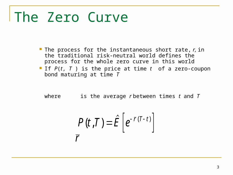
The process for the instantaneous short rate, r, in the traditional risk-neutral world defines the process for the whole zero curve in this world

If P(t, T ) is the price at time t of a zero-coupon bond maturing at time T

where is the average r between times t and T

P t T E e r T t( , ) ( )

r

4

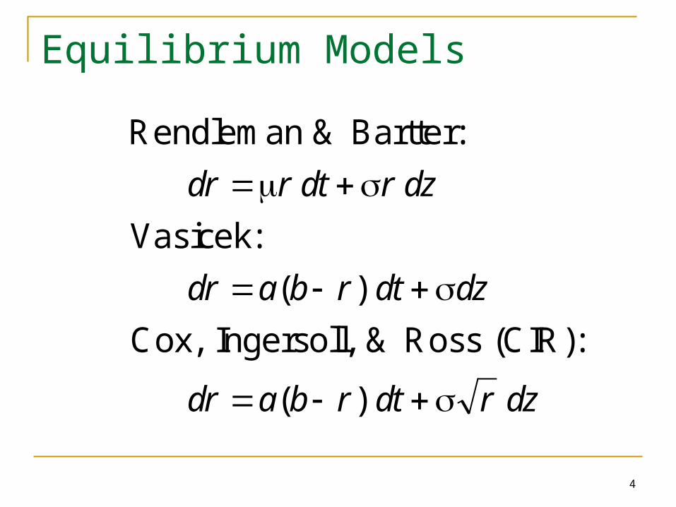
Equilibrium Models

Rendleman & Bartter:

Vasicek:

Cox, Ingersoll, & Ross (CIR):

dr r dt r dz

dr a b r dt dz

dr a b r dt r dz

( )

( )

5

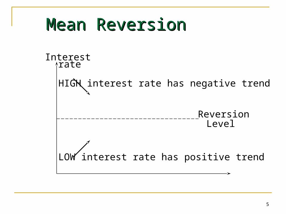
Mean Reversion Mean Reversion

Interestrate

HIGH interest rate has negative trend

LOW interest rate has positive trend

ReversionLevel

6

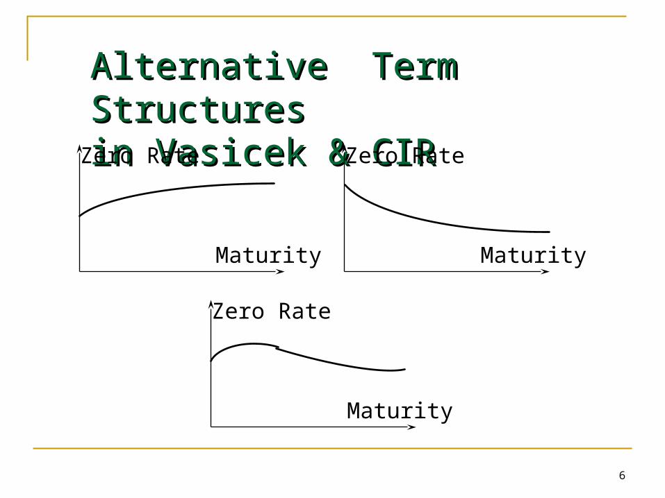
Alternative Term Alternative Term StructuresStructuresin Vasicek & CIR in Vasicek & CIR

Zero Rate

Maturity

Zero Rate

Maturity

Zero Rate

Maturity

Affine term structure models

Both Vasicek and CIR are affine term structure models

7

8

Equilibrium vs No-Arbitrage Models

In an equilibrium model today’s term structure is an output

In a no-arbitrage model today’s term structure is an input

9

Developing No-Arbitrage Model for r

A model for r can be made to fit the initial term structure by including a function of time in the drift

10

Ho-Lee Model

dr = (t)dt + dz Many analytic results for bond prices and

option prices Interest rates normally distributed One volatility parameter, All forward rates have the same standard

deviation

Diagrammatic Diagrammatic Representation of Ho-LeeRepresentation of Ho-Lee

11

Short Rate

r

r

r

rTime

12

Hull-White Model

dr = [(t ) – ar ]dt + dz Many analytic results for bond prices and option

prices Two volatility parameters, a and Interest rates normally distributed Standard deviation of a forward rate is a

declining function of its maturity

13

Diagrammatic Representation of Hull and White

Short Rate

r

r

r

rTime

Forward RateCurve

14

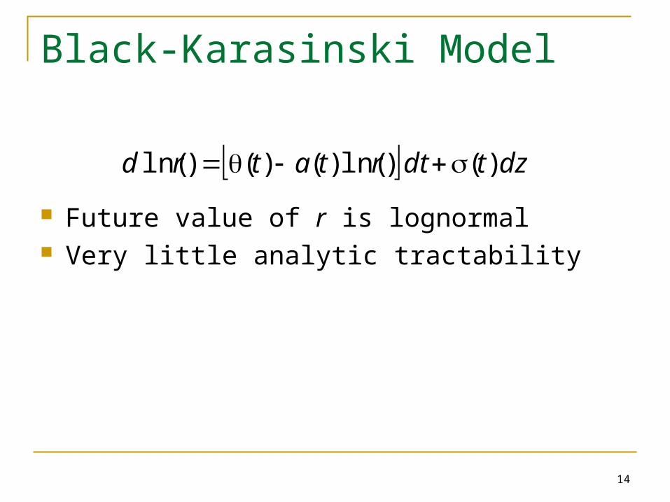
Black-Karasinski Model

Future value of r is lognormal Very little analytic tractability

dztdtrtatrd )()ln()()()ln(

15

Options on Zero-Coupon Bonds In Vasicek and Hull-White model, price of call maturing at T on a

bond lasting to s is

LP(0,s)N(h)-KP(0,T)N(h-P) Price of put is

KP(0,T)N(-h+P)-LP(0,s)N(h)

where

TTsσ

KL

a

ee

aKTP

sLPh

P

aTTsa

PP

P

)( Lee-HoFor

price. strike theis and principal theis

2

11

2),0(

),0(ln

1 2)(

16

Options on Coupon Bearing Bonds

In a one-factor model a European option on a coupon-bearing bond can be expressed as a portfolio of options on zero-coupon bonds.

We first calculate the critical interest rate at the option maturity for which the coupon-bearing bond price equals the strike price at maturity

The strike price for each zero-coupon bond is set equal to its value when the interest rate equals this critical value

17

Interest Rate Trees vs Stock Price Trees

The variable at each node in an interest rate tree is the t-period rate

Interest rate trees work similarly to stock price trees except that the discount rate used varies from node to node

18

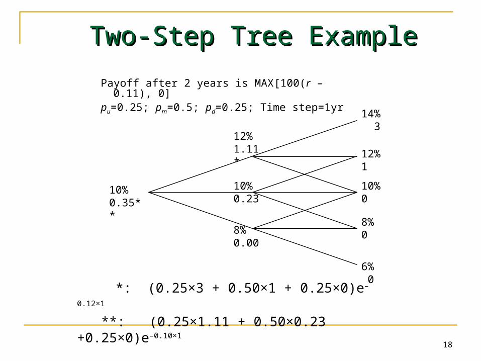
Two-Step Tree ExampleTwo-Step Tree Example

Payoff after 2 years is MAX[100(r – 0.11), 0]pu=0.25; pm=0.5; pd=0.25; Time step=1yr

10%0.35**

12% 1.11*

10% 0.23

8% 0.00

14% 3

12% 1

10% 0

8% 0

6% 0 *: (0.25×3 + 0.50×1 + 0.25×0)e–0.12×1

**: (0.25×1.11 + 0.50×0.23 +0.25×0)e–0.10×1

19

Alternative Branching Alternative Branching Processes in a Trinomial TreeProcesses in a Trinomial Tree

(a) (b) (c)

20

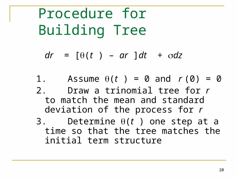
Procedure for Building Tree

dr = [(t ) – ar ]dt + dz

1.Assume (t ) = 0 and r (0) = 02.Draw a trinomial tree for r to match the

mean and standard deviation of the process for r

3.Determine (t ) one step at a time so that the tree matches the initial term structure

21

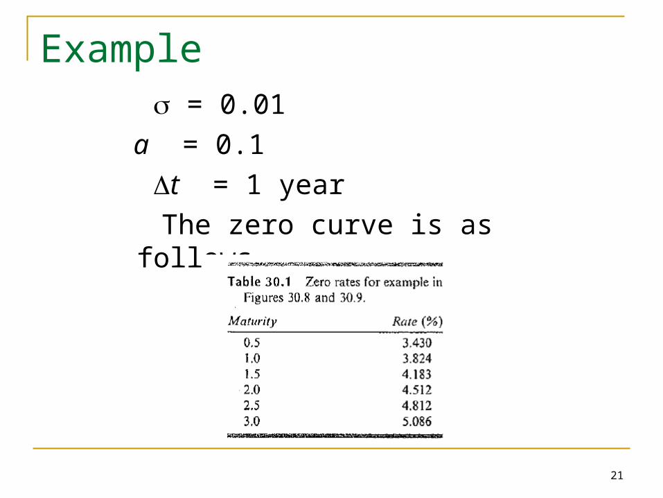
Example = 0.01

a = 0.1

t = 1 year

The zero curve is as follows

22

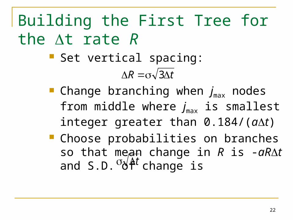
Building the First Tree for the t rate R

Set vertical spacing:

Change branching when jmax nodes from middle where jmax is smallest integer greater than 0.184/(at)

Choose probabilities on branches so that mean change in R is -aRt and S.D. of change is

tR 3

t

23

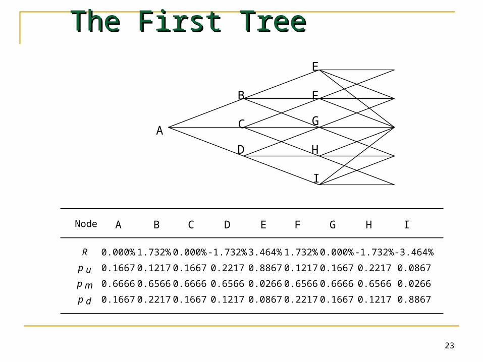
The First TreeThe First Tree

A

B

C

D

E

F

G

H

I

Node A B C D E F G H I

R 0.000% 1.732% 0.000% -1.732% 3.464% 1.732% 0.000% -1.732% -3.464%

p u 0.1667 0.1217 0.1667 0.2217 0.8867 0.1217 0.1667 0.2217 0.0867

p m 0.6666 0.6566 0.6666 0.6566 0.0266 0.6566 0.6666 0.6566 0.0266

p d 0.1667 0.2217 0.1667 0.1217 0.0867 0.2217 0.1667 0.1217 0.8867

24

Shifting Nodes

Work forward through tree Remember Qij the value of a derivative providing

a $1 payoff at node j at time it Shift nodes at time it by i so that the (i+1)t

bond is correctly priced

25

The Final TreeThe Final Tree

A

B

C

D

E

F

G

H

I

Node A B C D E F G H I

R 3.824% 6.937% 5.205% 3.473% 9.716% 7.984% 6.252% 4.520% 2.788%

p u 0.1667 0.1217 0.1667 0.2217 0.8867 0.1217 0.1667 0.2217 0.0867

p m 0.6666 0.6566 0.6666 0.6566 0.0266 0.6566 0.6666 0.6566 0.0266

p d 0.1667 0.2217 0.1667 0.1217 0.0867 0.2217 0.1667 0.1217 0.8867

26

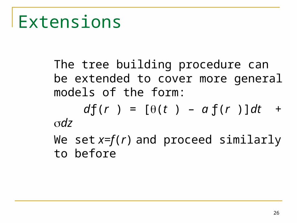
Extensions

The tree building procedure can be extended to cover more general models of the form:

dƒ(r ) = [(t ) – a ƒ(r )]dt + dz

We set x=f(r) and proceed similarly to before

27

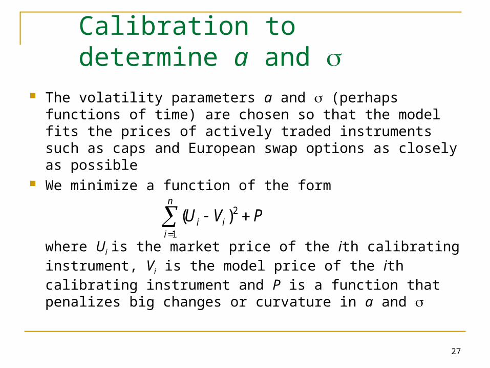
Calibration to determine a and

The volatility parameters a and (perhaps functions of time) are chosen so that the model fits the prices of actively traded instruments such as caps and European swap options as closely as possible

We minimize a function of the form

where Ui is the market price of the ith calibrating instrument, Vi is the model price of the ith calibrating instrument and P is a function that penalizes big changes or curvature in a and

n

iii PVU

1

2)(

HJM Model: NotationHJM Model: Notation

28

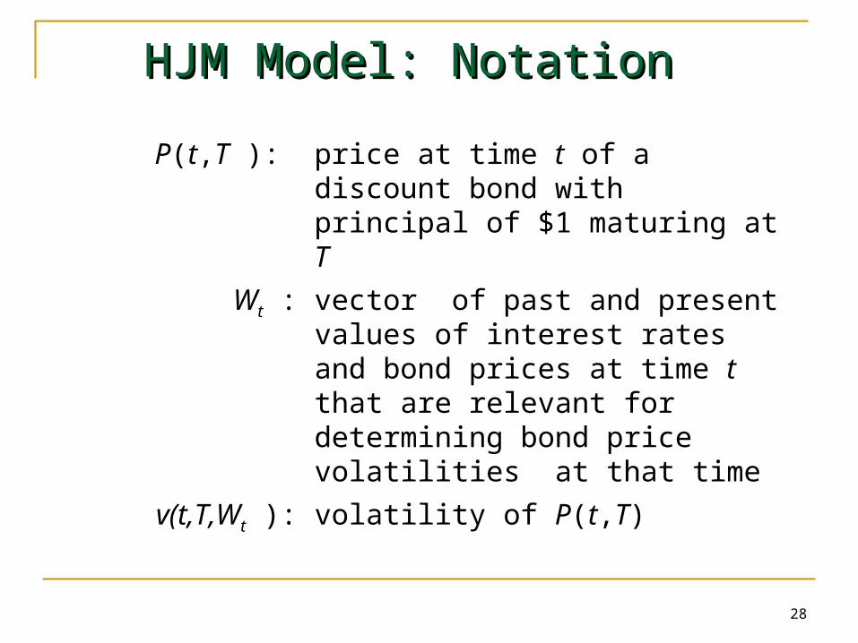
P(t,T ): price at time t of a discount bond with principal of $1 maturing at T

Wt : vector of past and present values of interest rates and bond prices at time t that are relevant for determining bond price volatilities at that time

v(t,T,Wt ): volatility of P(t,T)

Notation continuedNotation continued

29

ƒ(t,T1,T2): forward rate as seen at t for the period between T1 and T2

F(t,T): instantaneous forward rate as seen at t for a contract maturing at T

r(t): short-term risk-free interest rate at t

dz(t): Wiener process driving term structure movements

30

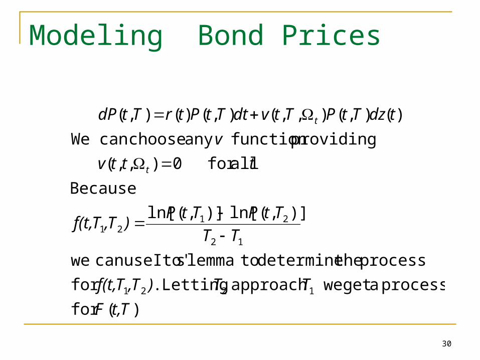
Modeling Bond Prices

) for

process a get we approach Letting for

process the determine to lemma sIto' use can we

Because

all for

providing function any choose can We

t,TF

TT),Tf(t,T

TT

TtPTtP),Tf(t,T

tttv

v

tdzTtPTtvdtTtPtrTtdP

t

t

(

.

)],(ln[)],(ln[

0),,(

)(),(),,(),()(),(

1221

12

2121

31

The process for The process for FF((tt,,TT))

factor one

than more is there whenhold results Similar

have must we

(),(

write weif that means result This

dτs(t,)ΩT,s(t,)ΩT, m(t,

)dzΩT,s(t,dtΩT,t,mTtdF

tdzTtvdtTtvTtvTtdF

T

t ttt

tt

tTtTt

),

)

)(),,(),,(),,(),(

32

Tree Evolution of Term Structure is Non-Recombining

Tree for the short rate r is non-Markov

33

The LIBOR Market Model

The LIBOR market model is a model constructed in terms of the forward rates underlying caplet prices

34

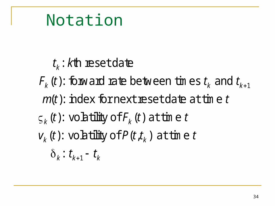
Notation

t k

F t t t

m t t

t F t t

v t P t t t

t t

k

k k k

k k

k k

k k k

: th reset date

forward rate between times and

: index for next reset date at time

volatility of at time

volatility of ( , at time

( ):

( )

( ): ( )

( ): )

:

1

1

35

Volatility Structure

We assume a stationary volatility structure

where the volatility of depends only on

the number of accrual periods between the

next reset date and [i.e., it is a function only

of ]

F t

t

k m t

k

k

( )

( )

36

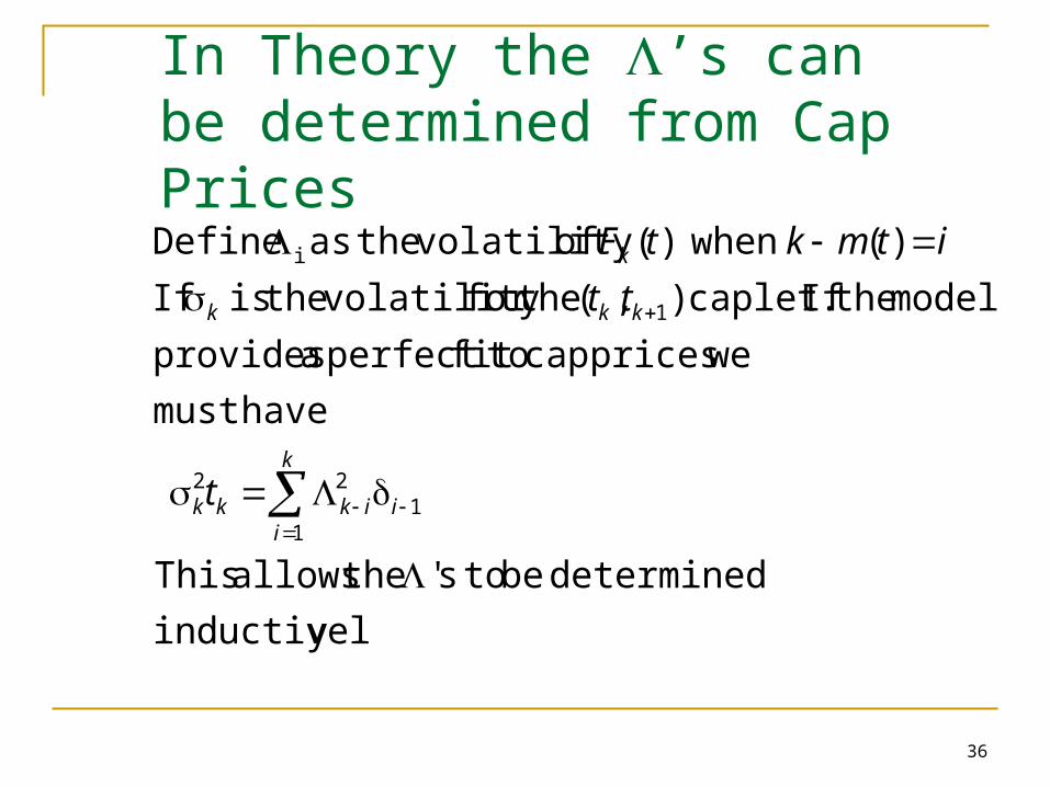
In Theory the ’s can be determined from Cap Prices

yinductivel

determined be to s the allows This

have must

weprices cap to fit perfect a provides

model the If caplet. the for volatility the is If

when of volatility the as Define i

'

),(

)()(

11

22

1

k

iiikkk

kkk

k

t

tt

itmktF

37

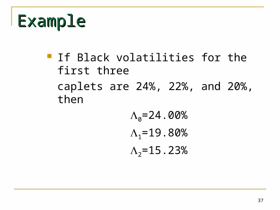
ExampleExample

If Black volatilities for the first three

caplets are 24%, 22%, and 20%, then

0=24.00%

1=19.80%

2=15.23%

38

ExampleExample

n 1 2 3 4 5

n(%) 15.50 18.25 17.91 17.74 17.27

n-1(%) 15.50 20.64 17.21 17.22 15.25

n 6 7 8 9 10

n(%) 16.79 16.30 16.01 15.76 15.54

n-1(%) 14.15 12.98 13.81 13.60 13.40

39

The Process for Fk in a One-Factor LIBOR Market Model

dF F dz

P t t

k k m t k

i

( )

( , ),

The drift depends on the world chosen

In a world that is forward risk -neutral

with respect to the drift is zero1

40

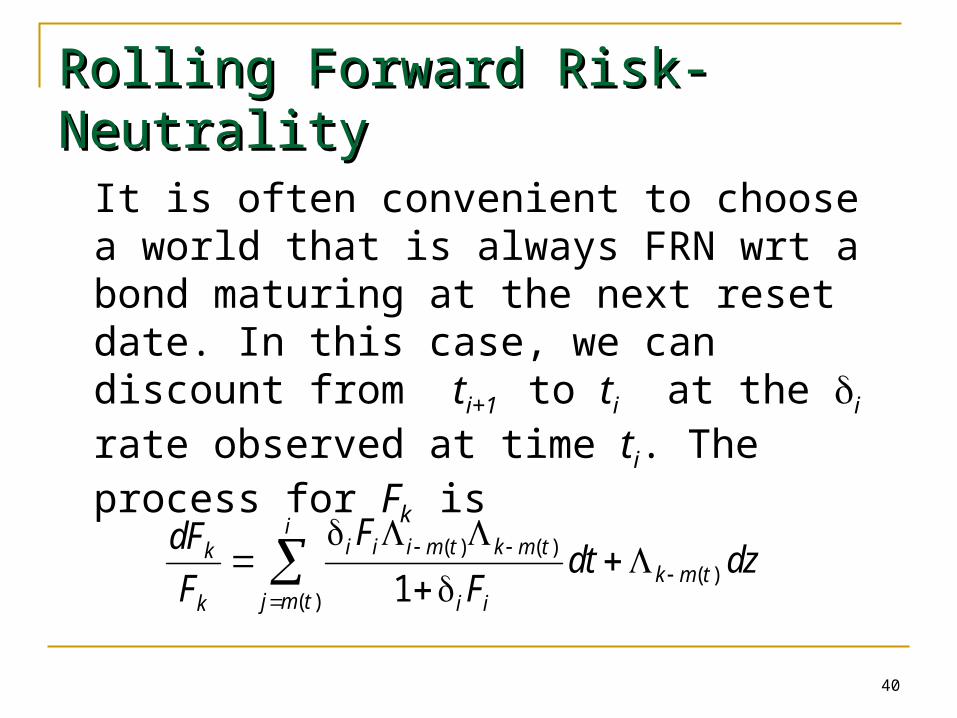
Rolling Forward Risk-Rolling Forward Risk-NeutralityNeutrality

It is often convenient to choose a world that is always FRN wrt a bond maturing at the next reset date. In this case, we can discount from ti+1 to ti at the i rate observed at time ti. The process for Fk is

dF

F

F

Fdt dzk

k

i i i m t k m t

i ij m t

i

k m t

( ) ( )

( )( )1

41

The LIBOR Market Model and HJM

In the limit as the time between resets tends to zero, the LIBOR market model with rolling forward risk neutrality becomes the HJM model in the traditional risk-neutral world

42

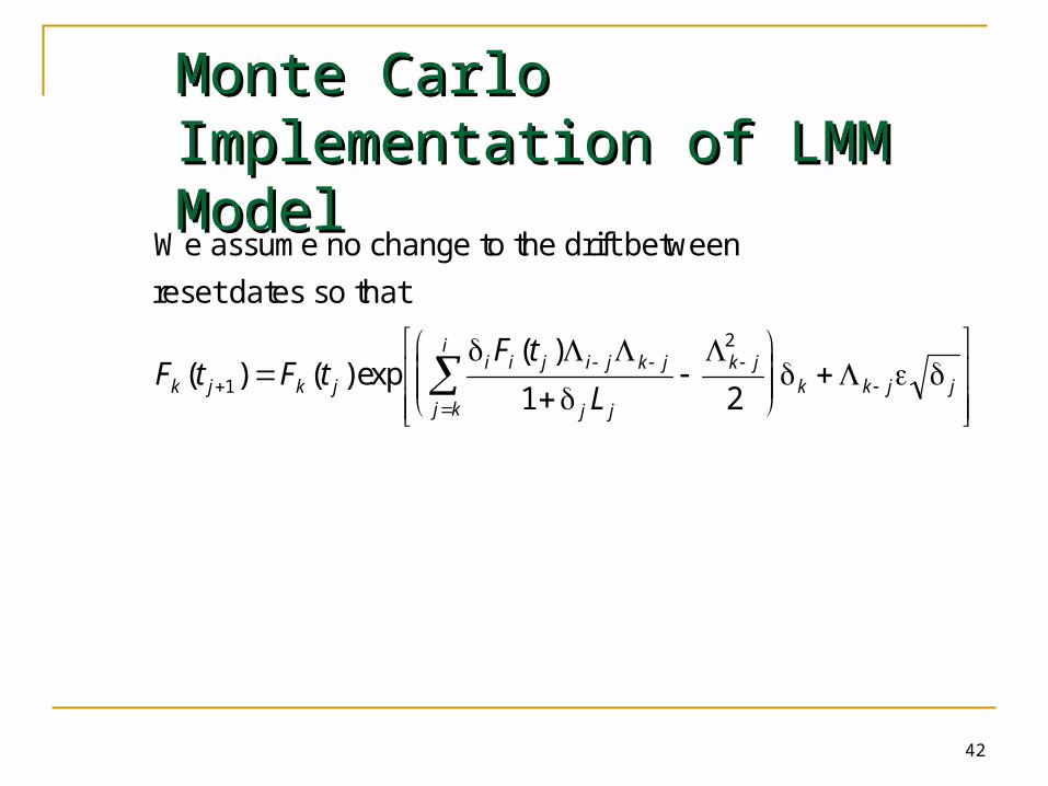
Monte Carlo Implementation Monte Carlo Implementation of LMM Model of LMM Model

We assume no change to the drift between

reset dates so that

F t F tF t

Lk j k ji i j i j k j

j j

k j

j k

i

k k j j( ) ( ) exp( )

1

2

1 2

43

Multifactor Versions of LMM

LMM can be extended so that there are several components to the volatility

A factor analysis can be used to determine how the volatility of Fk is split into components

44

Ratchet Caps, Sticky Caps, and Flexi Caps

A plain vanilla cap depends only on one forward rate. Its price is not dependent on the number of factors.

Ratchet caps, sticky caps, and flexi caps depend on the joint distribution of two or more forward rates. Their prices tend to increase with the number of factors

45

Valuing European Options in the LIBOR Market Model

There is an analytic approximation that can be used to value European swap options in the LIBOR market model.

46

Calibrating the LIBOR Market Model In theory the LMM can be exactly calibrated to

cap prices as described earlier In practice we proceed as for short rate models

to minimize a function of the form

where Ui is the market price of the ith calibrating instrument, Vi is the model price of the ith calibrating instrument and P is a function that penalizes big changes or curvature in a and

n

iii PVU

1

2)(

47

Types of Mortgage-Backed Securities (MBSs)

Pass-Through Collateralized Mortgage

Obligation (CMO) Interest Only (IO) Principal Only (PO)

48

Option-Adjusted Spread(OAS)

To calculate the OAS for an interest rate derivative we value it assuming that the initial yield curve is the Treasury curve + a spread

We use an iterative procedure to calculate the spread that makes the derivative’s model price = market price.

This spread is the OAS.