1. list the promise of ddbms . explain how ddbms provides the … · 2019-03-25 · a ddbs is not a...
TRANSCRIPT
Tulsiramji Gaikwad-Patil College of Engineering & Technology
Department of Master in Computer Application
Subject Notes
Academic Session: 2018 – 2019
Subject:DDBMS
Semester: I UNIT: I
1. List the promise of DDBMS . Explain how DDBMS provides
the separation of higher level semantics from lower level
implementation issues.
In previous sections we discussed various possible forms of transparency within a
distributed computing environment. Obviously, to provide easy and efficient access by
novice users to the services of the DBMS, one would want to have full transparency,
involving all the various types that we discussed. Nevertheless, the level of transparency
is inevitably a compromise between ease of use and the difficulty and overhead cost of
providing high levels of transparency.
What has not yet been discussed is who is responsible for providing these services. It
is possible to identify three discussed is who is responsible for providing these services. It
is possible to identify three distinct layers at which the services of transparency can be
provided. It is quite common to treat these as mutually exclusive means of providing the
service, although it is more appropriate to view them as complementary.
We could leave the responsibility of providing transparent access to data resources to
the access layer. the transparency features can be built into the user language, which then
translates the requested services into required operations. In other words, the complier or
the interpreter takes over the task and no transparent service is provided to the
implementer of the compiler or the interpreter.
The second layer at which transparency can be provided is the operating system level.
State-of-the-art operating systems provide some level of transparency to system users.
For example, the device drivers within the operating system handle the minute details of
getting each piece of peripheral equipment to do what is requested. The typical computer
user, or even an application programmer, does not normally write device drivers to
interact with individual peripheral equipment; that operation is transparent to the user.
Providing transparent access to resources at the operating system level can obviously
be extended to the distributed environment, where the management of the network
resource is taken over by the distributed operating system. This is a good level at which

to provide network transparency if it can be accomplished. The unfortunate aspect is that
not all commercially available distributed operating systems provide a reasonable level of
transparency in network management.
The third layer at which transparency can be supported is within the DBMS. The
transparency and support for database functions provided to the DBMS designers by an
underlying operating system is generally minimal and typically limited to very
fundamental operations for performing certain tasks. It is the responsibility of the DBMS
to make all the necessary translation from the operating system to the higher-level user
interface. This mode of operation is the most common method today. There are, however,
various problems associated with the interaction of the operating system with the
distributed DBMS and are discussed throughout this book.
It is therefore quite important to realize that reasonable levels of transparency
depend on different components within the data management environment. Network
transparency can easily be handled by the distributed operating system part of its
responsibilities for providing replication and fragmentation transparencies (especially
those aspects dealing with transaction management and recovery). The DBMS should be
responsible for providing a high level of data independence together with replication and
fragmentation transparencies. Finally, the user interface can support a higher level of
transparency not only in terms of a uniform access method to the data resources from
within a language. But also in terms of structure constructs that permit the user to deal
with objects in his or her environment rather than focusing on the details of database
description. Specifically, it should be noted that the interface to a distributed DBMS does
not need to be a programming language but can be a graphical user interface, a natural
language interface, and even a voice system.
A hierarchy of these transparencies is shown in Figure. It is not always easy to
delineate clearly the levels of transparency, but such a figure serves an important
instructional purpose even if it is not fully correct. To complete the picture we have
added a “language transparency” layer, although it is not discussed in this chapter. With
this generic layer, users have high-level access to the data (e.g., fourth-generation
languages, graphical user interfaces, natural language access).

How Do Existing Systems Fare
Most of the commercial distributed DBMSs today have started to provided some level of
transparency support. Typically the systems provide distribution transparency, support
for horizontal fragmentation and some form of replication transparency.
This level of support is quite recent. Until recently, most commercial distributed
DBMSs did not provide a sufficient level of transparency. Some (e.g., R* [Williams et al.
1982]) required users to embed the location names within the name of each database
object. Furthermore, they required the user to specify the full name for access to the
object. Obviously, one can set up aliases for these long names if the operating system
provides such a facility. However, user-defined aliases are not real solutions to the
problem in as much as they are attempts to avoid addressing them within the distributed
DBMS. The system, not the user, should be responsible for assigning unique names to
objects and for translating user-known names to these unique internal object names.
Besides these semantic considerations, there is also a very pragmatic problem
associated with embedding location names within object names. Such an approach makes
it very difficult to move objects across machines for performance optimization or other
purposes. Every such move will require users to change their access names for the
affected objects, which is clearly undesirable.
Other systems did not provide any support for the management of replicate data
across multiple logical databases. Even those that did required that the user be physically
“logged on” to one database at a given time (e.g., Oracle versions prior to V7).

At this point it is important to point out that full transparency is not a universally
accepted objective. Gray argues that full transparency makes the management of
distributed data very difficult and claims that “applications coded with transparent access
to geographically distributed databases have: poor manage-ability, poor modularity, and
poor message performance”. He proposes a remote procedure call mechanism between
the requestor users and the server DBMSs whereby the users would direct their queries to
a specific DBMS. It is indeed true that the management of distributed data is more
difficult if transparent access is provided to users, and that the client/server architecture
(which we discuss in Chapter 4) with a remote procedure call-based communication
between the clients and the servers is the tight architectural approach. In fact, some
commercial distributed DBMSs are organized in this fashion. However, the goal of fully
transparent access to distributed and replicated data is an important one and it is up to the
system vendors to resolve the system issues.
2. Is there any similarities between multiprocessor and
distributed database system ? If yes , explain how.
DISTRIBUTED DATA PROCESSING
The term of distributed processing (or distributed computing) is probably the most
abused term in computer science of the last couple of years. It has been used to refer to
such diverse systems as multiprocessor systems, distributed data processing, and
computer networks. This abuse has gone on to such an extent that the term distributed
processing has sometimes been called “a concept in search of a definition and a name.”
Here are some of the other terms that have been used synonymously with distributed
processing: distributed function, distributed computers or computing, networks,
multiprocessors/multicomputers, satellite processing/satellite computers, backend
processing, dedicated/special-purpose computers, time-shared systems, and functionally
modular systems.
Obviously, some degree of distributed processing goes on in any computer system,
even on single-processor computers. Starting with the second-generation computers, the
central processing unit (CPU) and input/output (I/O) functions have been separated and
overlapped. This separation and overlap can be considered as one form of distributed
processing. However, it should be quite clear that what we would like to refer to as
distributed processing, or distributed computing, has nothing to do with this form of
distribution of functions in a single-processor computer system.
A term that has caused so much confusion is obviously quite difficult to define
precisely. There have been numerous attempts to define what distributed processing is,
and almost every researcher has come up with a definition. In this book we define

distributed processing in such a way that it leads to a definition of what a distributed
database system is. The working definition we use for a distributed computing system
states that it is a number of autonomous processing elements (not necessarily
homogeneous) that are interconnected by a computer network and that cooperate in
performing their assigned tasks. The “processing element” referred to in this definition is
a computing device that can execute a program on its own.
One fundamental question that needs to be asked is: What is being distributed? One
of the things that might be distributed is the processing logic. In fact, the definition of a
distributed computing system given above implicitly assumes that the processing logic or
processing elements are distributed. Another possible distribution is according to
function. Various functions of a computer system could be delegated to various pieces of
hardware or software. A third possible mode of distribution is according to data. Data
used by a number of applications may be distributed to a number of processing sites.
Finally, control can be distributed. The control of the execution of various tasks might be
distributed instead of being performed by one computer system. From the viewpoint of
distributed database systems, these modes distribution are all necessary and important. In
the following sections we talk about these in more detail.
We can define a distributed database as a collection of multiple, logically interrelated
databases distributed over a computer network. A distributed database management
system (distributed DBMS) is then defined as the software system that permits the
management of the DDBS and makes the distribution transparent to the users. The two
important terms in thee definitions are “logically interrelated” and “distributed over a
computer network.” They help eliminate certain cases that have sometimes been accepted
to represent a DDBS.
A DDBS is not a “collection of files” that can be individually stored at each node of a
computer network. To form a DDBS, files should not only be logically related, but there
should be structure among the files, and access should be via a common interface. We
should note that there has been much recent activity in providing DBMS functionality
over semi-structured data that are stored in files on the Internet (such as Web pages). In
light of this activity, the above requirement may seem unnecessarily strict. However,
providing “DBMS-like” access to data is different than a DDBS:
It has sometimes been assumed that the physical distribution of data is not the most
significant issue. The proponents of this view would therefore feel comfortable in
labeling as a distributed database two (related) databases that that reside in the same
computer system. However, the physical distribution of data is very important. It creates
problems that are not encountered when the databases reside in the same computer. Note
that physical distribution does not necessarily imply that the computer systems be
geographically far apart; they could actually be in the same room. It simply implies that
the communication between them is done over a network instead of through shared
memory, with the network as the only shared resource.
This brings us to another point. The definition above also rules out multiprocessor
systems as DDBSs. A multiprocessor system is generally considered to be a system
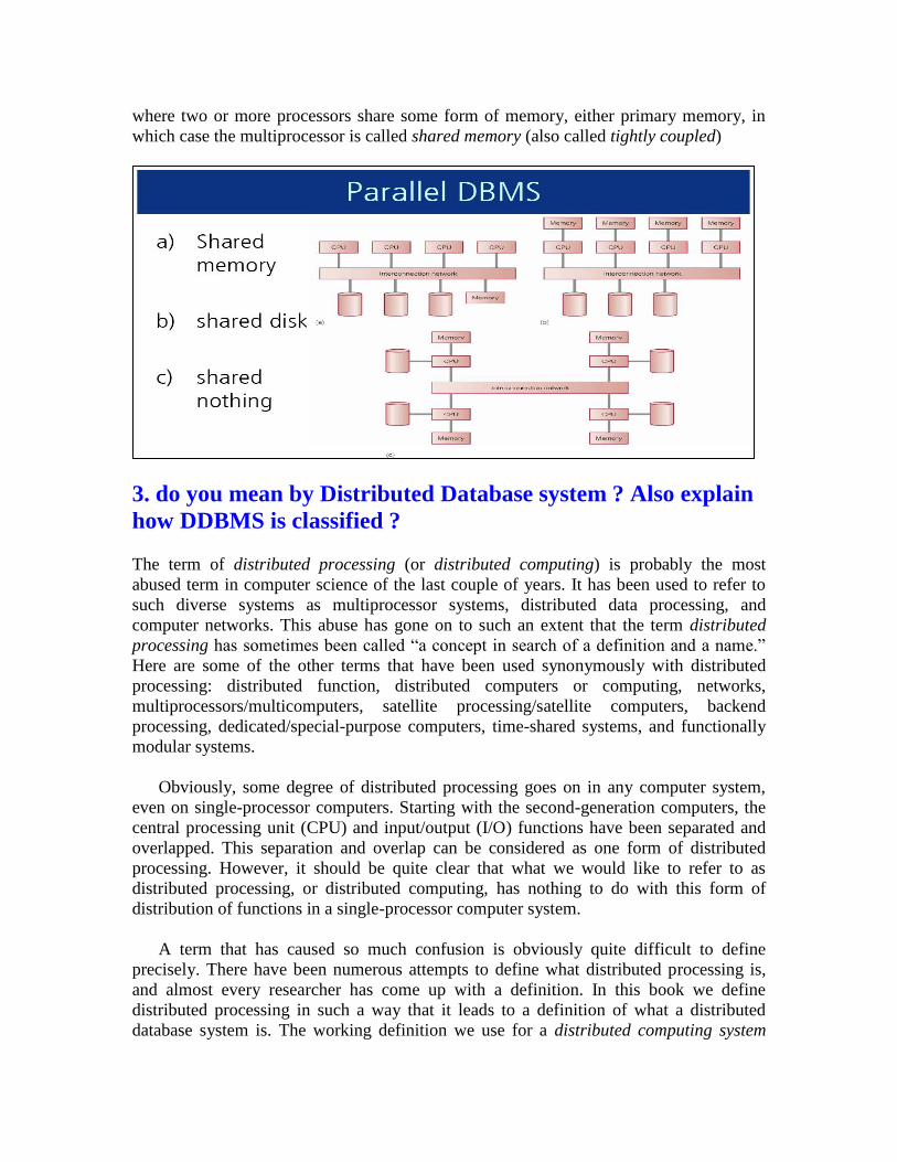
where two or more processors share some form of memory, either primary memory, in
which case the multiprocessor is called shared memory (also called tightly coupled)
3. do you mean by Distributed Database system ? Also explain
how DDBMS is classified ?
The term of distributed processing (or distributed computing) is probably the most
abused term in computer science of the last couple of years. It has been used to refer to
such diverse systems as multiprocessor systems, distributed data processing, and
computer networks. This abuse has gone on to such an extent that the term distributed
processing has sometimes been called “a concept in search of a definition and a name.”
Here are some of the other terms that have been used synonymously with distributed
processing: distributed function, distributed computers or computing, networks,
multiprocessors/multicomputers, satellite processing/satellite computers, backend
processing, dedicated/special-purpose computers, time-shared systems, and functionally
modular systems.
Obviously, some degree of distributed processing goes on in any computer system,
even on single-processor computers. Starting with the second-generation computers, the
central processing unit (CPU) and input/output (I/O) functions have been separated and
overlapped. This separation and overlap can be considered as one form of distributed
processing. However, it should be quite clear that what we would like to refer to as
distributed processing, or distributed computing, has nothing to do with this form of
distribution of functions in a single-processor computer system.
A term that has caused so much confusion is obviously quite difficult to define
precisely. There have been numerous attempts to define what distributed processing is,
and almost every researcher has come up with a definition. In this book we define
distributed processing in such a way that it leads to a definition of what a distributed
database system is. The working definition we use for a distributed computing system

states that it is a number of autonomous processing elements (not necessarily
homogeneous) that are interconnected by a computer network and that cooperate in
performing their assigned tasks. The “processing element” referred to in this definition is
a computing device that can execute a program on its own.
One fundamental question that needs to be asked is: What is being distributed? One
of the things that might be distributed is the processing logic. In fact, the definition of a
distributed computing system given above implicitly assumes that the processing logic or
processing elements are distributed. Another possible distribution is according to
function. Various functions of a computer system could be delegated to various pieces of
hardware or software. A third possible mode of distribution is according to data. Data
used by a number of applications may be distributed to a number of processing sites.
Finally, control can be distributed. The control of the execution of various tasks might be
distributed instead of being performed by one computer system. From the viewpoint of
distributed database systems, these modes distribution are all necessary and important. In
the following sections we talk about these in more detail.
We can define a distributed database as a collection of multiple, logically interrelated
databases distributed over a computer network. A distributed database management
system (distributed DBMS) is then defined as the software system that permits the
management of the DDBS and makes the distribution transparent to the users. The two
important terms in thee definitions are “logically interrelated” and “distributed over a
computer network.” They help eliminate certain cases that have sometimes been accepted
to represent a DDBS.
4. How could you relate the problem areas of DDBMS?

Relationship among Problems
We should mention at this point that these problems are not isolated from one another.
The reasons for studying them in isolation are that (1) problems are difficult enough to
study by themselves, and would probably be impossible to present all together, and that
(2) it might be possible to characterize the effect of one problem on another one, through
the use of parameters and constraints. In fact, each problem is affected by the solutions
found for the others, and in turn affects the set of feasible solutions for them. In this
section we discuss how they are related.
The relationship among the components is shown in Figure. The design of distributed
databases affects many areas. It affects directory management, because the definition of
fragments and their placement determine the contents of the directory (or directories) as
well as the strategies that may be employed to manage them. The same information (i.e.,
fragment structure and placement) is used by the query processor to determine the query
evaluation strategy. On the other hand, the access and usage patterns that are determined
by the query processor are used as inputs to the data distribution and fragmentation
algorithms. Similarly, directory placement and contents influence the processing of
queries.
The replication of fragments when they are distributed affects the concurrency control
strategies that might be employed, some concurrency control algorithms cannot be easily
used with replicated databases. Similarly, usage and access patterns to the database will
influence the concurrency control algorithms. If the environment is update intensive, the
necessary precautions are quite different from those in a query-only environment.

There is a strong relationship among the concurrency control problem, the deadlock
management problem, and reliability issues. This is to be expected, since together they
are usually called the reliability issues. This is to be expected, since together they usually
called the transaction management problem. The concurrency control algorithm that is
employed will determine whether or not a separate deadlock management facility is
required. If a locking-based algorithm is used, deadlocks will occur, whereas they will
not if timestamping is the chosen alternative.
Reliability mechanisms are implemented on top of a concurrency control algorithm.
Therefore, the relationship among them is self-explanatory. It should also be mentioned
that the reliability mechanisms being considered have an effect on the choice of the
concurrency control algorithm. Techniques to provided reliability also make use of data
placement information since the existence of duplicate copies of the data serve as a
safeguard to maintain reliable operation.
Two of the problems we discussed in the preceding sections—operating system issues
and heterogeneous databases—are not illustrated in Figure.This is obviously not because
they have no bearing on other issues; in fact, exactly the opposite is true. The type of
operating system used and the features supported by that operating system greatly
influence what solution strategies can be applied in any of the other problem areas.
Similarly, the nature of all these problems change considerably when the environment is
heterogeneous. The same issues have to be dealt with differently when the machine
architecture, the operating systems, and the local database management software vary
from site to site.
Unit II
1. Write an algorithm for derived horizontal fragmentation. Derived Horizontal Fragmentation
A derived horizontal fragmentation is defined on a member relation of a link according to
a selection operation specified on its owner. It is important to remember two points. First,
the link between the owner and the member relations is defined as an equi-join. Second,
an equi-join can be implemented b means of semijoins. This second point is especially
important for our purposes, since we want to partition a member relation according to the
fragmentation of its owner, but we also want the resulting fragment to be defined only on
the attributes of the member relation.
Accordingly, given a link L where owner (L) = S and member (L) = R, the derived
horizontal fragments of R are defined as
Ri = R Si, 1 i w

where w is the maximum number of fragments that will be defined on R, and
Si = σ Fi,(S), where Fi is the formula according to which the primary horizontal fragment
Si is defined.
Example
Consider, where owner (L1) = PAY and member (L1) = EMP. Then we can group
engineers into two groups according to their salary: those making less than or equal to
$30,000, and those making more than $30,000. The two fragments EMP1 and EMP2
are defined as follows:
EMP1 = EMP PAY1
EMP2 = EMP PAY2
where
PAY1 = σ SAL 30000(PAY)
PAY2 = σ SAL >30000(PAY)
The result of this fragmentation is depicted in Figure 5.11.
To carry out a derived horizontal fragmentation, three inputs are needed: the set of
partitions of the owner relation (e.g., PAY1 and PAY2 in Example 5.12), the member
relation, and the set of semijoin predicates between the owner and the member (e.g.,
EMP.TITLE = PAY.TITLE in Example). The fragmentation algorithm, then is quite
trivial, so we will not present it in any detail.
There is one potential complication that deserves some attention. In a database
schema, it is common that there are more than two links into a relation R . In this case
there is more than one possible derived horizontal fragmentation of R. the decision as to
which candidate fragmentation to choose is based on two criteria:
1. The fragmentation with better join characteristic
2. the fragmentation used in more applications.
Let us discuss the second criterion first. This is quite straightforward if we take into
consideration the frequency with which applications access some data. If possible, one
should try to facilitate the accesses of the “heavy” users so that their total impact on
system performance is minimized.
Applying the first criterion, however, is not that straightforward. Consider, for
example, the fragmentation we discussed in Example. The effect (and the objective) of
this fragmentation is that the join of the EMP and PAY relations to answer the query is
assisted (1) by performing it on smaller relations (i.e., fragments), and (2) by potentially
performing joins in a distributed fashion.

The first point is obvious. The fragments of EMP are smaller than EMP itself.
Therefore, it will be faster to join any fragment of PAY with any fragment of EMP than
to work with the relations themselves. The second point, however, is more important and
is at the heart of distributed databases. If, besides executing a number of queries at
different sites, we can execute one query in parallel, the response time or throughput of
the system can be expected to improve. In the case of joins, this is possible under certain
circumstances. Consider, for example, the join graph (i.e., the links) between the
fragments of EMP and PAY derived in Example. There is only one link coming in or
going out of a fragment. Such a join graph is called a simple graph. The advantage of a
design where the join relationship between fragments is simple is that the member and
owner of a link can be allocated to one site and the joins between different pairs of
fragments can proceed independently and in parallel.
Unfortunately, obtaining simple join graphs may not always be possible. In that case,
the next desirable alternative is to have a design that results in a partitioned join graph. A
partitioned graph consists of two or more subgraphs with no links between them.
Fragments so obtained may not be distributed for parallel execution as easily as those
obtained via simple join graphs, but the allocation is still possible.
Example
Let us continue with the distribution design of the database we started in Example.
We already decided on the fragmentation of relation EMP according to the
fragmentation of PAY. let us now consider ASG. Assume that there are the following
two applications:
1. The first application finds the names of engineers who work at certain places.
It runs on all three sites and accesses the information about the engineers who
work on local projects with higher probability than those of projects at other
locations.
2. At each administrative site where employee records are managed, users would
like to access the projects that these employees work on and learn how long
they will work on those projects.
The first application results in a fragmentation of ASG according to the fragments
PROJ1, PROJ3, PROJ4 and PROJ6 of PROJ obtained in Example. Remember that
PROJ1: σLOC = “Montreal” BUDGET 200000(PROJ)
PROJ3: σLOC = “New York” BUDGET 200000(PROJ)
PROJ4: σLOC = “New York”) BUDGET > 200000(PROJ)
PROJ6: σLOC = “Paris”) BUDGET > 200000(PROJ)
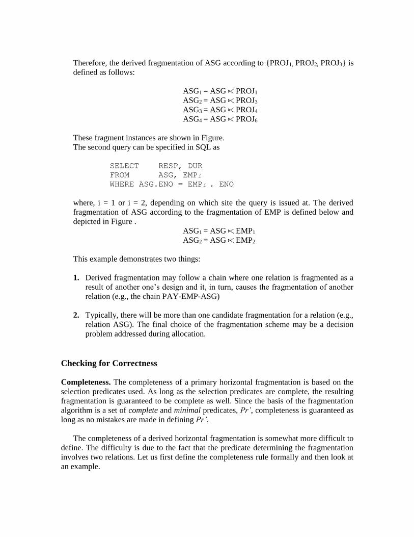
Therefore, the derived fragmentation of ASG according to {PROJ1, PROJ2, PROJ3} is
defined as follows:
ASG1 = ASG PROJ1
ASG2 = ASG PROJ3
ASG3 = ASG PROJ4
ASG4 = ASG PROJ6
These fragment instances are shown in Figure.
The second query can be specified in SQL as
SELECT RESP, DUR
FROM ASG, EMP i WHERE ASG.ENO = EMP i . ENO
where, i = 1 or i = 2, depending on which site the query is issued at. The derived
fragmentation of ASG according to the fragmentation of EMP is defined below and
depicted in Figure .
ASG1 = ASG EMP1
ASG2 = ASG EMP2
This example demonstrates two things:
1. Derived fragmentation may follow a chain where one relation is fragmented as a
result of another one’s design and it, in turn, causes the fragmentation of another
relation (e.g., the chain PAY-EMP-ASG)
2. Typically, there will be more than one candidate fragmentation for a relation (e.g.,
relation ASG). The final choice of the fragmentation scheme may be a decision
problem addressed during allocation.
Checking for Correctness
Completeness. The completeness of a primary horizontal fragmentation is based on the
selection predicates used. As long as the selection predicates are complete, the resulting
fragmentation is guaranteed to be complete as well. Since the basis of the fragmentation
algorithm is a set of complete and minimal predicates, Pr’, completeness is guaranteed as
long as no mistakes are made in defining Pr’.
The completeness of a derived horizontal fragmentation is somewhat more difficult to
define. The difficulty is due to the fact that the predicate determining the fragmentation
involves two relations. Let us first define the completeness rule formally and then look at
an example.

Let R be the member relation of a link whose owner is relation S, which is fragmented
as Fs = {S1, S2, …, Sw}. Furthermore, let A be the join attribute between R and S. Then for
each tuple t of R, there should be a tuple t of S such that
t [A] = t’ [A]
For example, there should be no ASG tuple which has a project number that is not
also contained in PROJ. Similarly, there should be no EMP tuples with TITLE values
where the same TITLE value does not appear in PAY as well. This rule is known as
referential integrity and ensures that the tuples of any fragment of the member relation
are also in the owner relation.
Reconstruction. Reconstruction of a global relation from its fragments is performed by
the union operator in both the primary and the derived horizontal fragmentation. Thus,
for a relation R with fragmentation
R = Ri, Ri FR
Disjointness. It is easier to establish Disjointness of fragmentation for primary than for
derived horizontal fragmentation. In the former ease, disjointness is guaranteed as long as
the minterm predicates determining the fragmentation are mutually exclusive.
In derived fragmentation, however, there is a semijoin involved that adds
considerable complexity. Disjointness can be guaranteed If the join graph is simple. If it
is not simple, it is necessary to investigate actual tuple values. In general, we do not want
a tuple of a member relation to join with two or more tuples of the owner relation when
these tuples are in different fragments of the owner. This may not be very easy to
establish, and illustrates why derived fragmentation schemes that generate a simple join
graph are always desirable.
Example 5.14
In fragmenting relation PAY the minterm predicates M = {1m ,
2m } were
1m : SAL 30000
2m : SAL > 30000
Since 1m and 2m are mutually exclusive, the fragmentation of PAY is disjoint. For
relation EMP, however, we require that
1. Each engineer have a single title.
2. Each title have a single salary value associated with it.
Since these two rules follow from the semantics of the database, the fragmentation of
EMP with respect to PAY is also disjoint.

2. Explain the MDBS architecture with GCS and without GCS
and explain how GCS is different in MDBS than DDBMs. MDBS Architecture
The differences in the level of autonomy between the distributed multi-DBMSs and
distributed DBMSs are also reflected in their architectural models. The fundamental
difference relates to the definition of the global conceptual schema. In the case of
logically integrated distributed DBMSs, the global conceptual schema defines the
conceptual view of the entire database, while in the case of distributed multi-DBMSs, it
represents only the collection of some of the local databases that each local DBMS wants
to share. Thus the definition of a global database is different in MDBSs than in
distributed DBMSs. In the latter, the global database is equal to the union of local
databases, whereas in the former it is only subset of the same union. There are even
arguments as to whether the global conceptual schema should even exist in multidatabase
systems. This question forms the basis of our architectural discussions in this section.
Module Using a Global Conceptual Schema
In an MDBS, the GCS is defined by integrating either the external schemas of local
autonomous databases or parts of their local conceptual schemas. Furthermore, users of a
local DBMS define their own views on the local database and do not need to change their
applications if they do not want to access data from another database. This is again an
issue of autonomy.
Designing the global conceptual schema in multidatabase systems involves the
integration of either the local conceptual schemas or the local external schemas. A major
difference between the design of the GCS in multi-DBMSs and in logically integrated
distributed DBMSs is that in the former the mapping is from local conceptual schemas to
a global schema. In the latter, however, mapping is in the reverse direction. As we
discuss in Chapter 5, this is because the design in the former is usually a bottom-up
process, whereas in the latter it is usually a top-down procedure. Furthermore, if
heterogeneity exists in the multidatabase system, a canonical data model has to be found
to define the GCS.

Once the GCS has been designed, views over the global schema can be defined for
users who require global access. It is not necessary for the GES and GCS to be defined
using the same data model and language; whether they do or not determines whether the
system is homogeneous or heterogeneous.
If heterogeneity exists in the system, then two implementation alternatives exist:
unilingual and multilingual. A unilingual multi-DBMS requires the users to utilize
possibly different data models and languages when both a local database and the global
database are accessed. The identifying characteristic of unilingual systems is that any
application that accesses data from multiple databases must do so by means of an external
view that is defined on the global conceptual schema. This means that the user of the
global database is effectively a different user than those who access only a local database,
utilizing a different data model and a different data language. Thus, one application may
have a local external schema (LES) defined on the local conceptual schema as well as a
global external schema (GES) defined on the global conceptual schema. The different
external view definitions may require the use of different access languages. Figure
actually depicts the datalogical model of a unilingual database system that integrates the
local conceptual schemas (or parts of them) into a global conceptual schema. Examples
of such an architecture are the MULTIBASE.
An alternative is multilingual architecture where the basic philosophy is to permit
each user to access the global database (i.e., data from other databases) by means of an
external schema, defined using the language of the user’s local DMBS. The GCS

definition is quite similar in the multilingual architecture and the unilingual approach, the
major difference being the definition of the external schemas’ which are described in the
language of external schemas of the local database. Assuming that the definition is purely
local, a query issued according to a particular schema is handled exactly as query in the
centralized DBMSs. Queries, against the global database are made using the language of
the local DMBS, but they generally require some processing to be mapped to the global
conceptual schema.
Models Without a Global Conceptual Schema
The existence of a global conceptual schema in a multidatabase system is a controversial
issue. There are researchers who even define a multidatabase management system as one
that manages “several databases without a global schema” It is argued that the absence of
a GCS is a significant advantage of multidatabase systems over distributed database
systems. One prototype system that has used this architectural model is the MRDSM
project The architecture depicted in Figure 4.9, identifies two layers: the local system
layer and the multidatabase layer on top of it. The local system layer consists of a number
of DBMSs, which present to the multidatabase layer the part of their local database they
are willing to share with users of other databases. This shared data is presented either as
the actual local conceptual schema or as a local external schema definition. If
heterogeneity is involved, each of these schemas, LCSi, may use a different data model.
Above this layer, external views are constructed where each view may be defined on
one local conceptual schema or on multiple conceptual schemas. Thus the responsibility
of providing access to multiple (and may be heterogeneous) databases is delegated to the
mapping between the external schemas and the local conceptual schemas. This is
fundamentally different from architectural models that use a global conceptual schema,
where this responsibility is taken over by the mapping between the global conceptual

schema and the local ones. This shift in responsibility has a practical consequence.
Access to multiple databases is provided by means of a powerful language in which user
applications are written.
Federated database architectures, which we discussed briefly, do not use a global
conceptual schema either. In the specific system described in, each local DBMS defines
an export schema, which describes the data it is willing to share with others. In the
terminology that we have been using, the global database is the union of all the export
schemas. Each, application that accesses, the global database does so by the definition of
an import schema, which is simply a global external view.
The component-based architectural model of a multi-DBMS is significantly different
from a distributed DBMS. The fundamental difference is the existence of full-fledged
DBMSs, each of which manages a different database. The MDBS provides a layer of
software that runs on top of these individual DBMSs and provides users with the facilities
of accessing various databases .Depending on the existence (or lack of it), the contents of
this layer of software would change significantly. Note that Figure represents a
nondistributed multi-DBMS. If the system is distributed, we would need to replicate the
multidatabase layer to each site where there is a local DBMS that participates in the
system. Also note that as far as the individual DBMSs are concerned, the MDBS layer is
simply another application that submits requests and receives answers.
The domain of federated database and multidatabase systems is complicated by the
proliferation of terminology and different architectural models. We bring some order to
the field in this section, but the architectural approaches that we summarize are not
unique.
3. Explain structural and functional implementation of “ANSI |
x3| SPARC” DBMS frame work.
In late 1972, the Computer and Information Processing Committee (X3) of the
American National Standards Institute (ANSI) established a Study Group on Database
Management Systems under the auspices of its Standards Planning and Requirements
Committee (SPARC). The mission of the study group was to study the feasibility of
setting up standards in this area, as well as determining which aspects should be
standardized if it was feasible. The study group issued its interim report in 1975 [SPARC,
1975], and its final report in 1977. The architectural framework proposed in these reports
came to be known as the “ANSI/SPARC architecture,” its full title being
“ANSi/X3/SPARC DBMS Framework.” The study group proposed that the interfaces be
standardized, and defined an architectural framework that contained 43 interfaces, 14 of
which would deal with the physical storage subsystem of the computer and therefore not
be considered essential parts of the DBMS architecture.
With respect to our earlier discussion on alternative approaches to standardization, the
ANSI/SPARC architecture is claimed to be based on the data organization. It recognizes
three views of data: the external view, which is that of the user, who might be a
programmer; the internal view, that of the system or machine; and the conceptual view,
that of the enterprise. For each of these views, an appropriate schema definition is
required. Figure depicts the ANSI/SPARC architecture from the data organization
perspective.
At the lowest level of the architecture is the internal view, which deals with the
physical definition and organization of data. The location of data on different storage
devices and the access mechanisms used to reach and manipulate data are the issues dealt
with at this level. At the other extreme is the external view, which is concerned with how
users view the database. An individual user’s view represents the portion of the database
that will be accessed by that user as well as the relationships that the user would like to
see among the data. A view can be shared among a number of users, with the collection
of user views making up the external schema. In between these two ends is the
conceptual schema, which is an abstract definition of the database. It is the “real world”
view of the enterprise being modeled in the database . As such, it is supposed to represent
the data and the relationships among data without considering the requirements of
individual applications or the restrictions of the physical storage media. In reality,
however, it is not possible to ignore these requirements completely, due to performance
reasons. The transformation between these three levels is accomplished by mappings that
specify how a definition at one level can be obtained from a definition at another level.

Example
Let us consider the engineering database example we have been using and indicate
how it can be described using a fictitious DBMS that conforms to the ANSI/SPARC
architecture. Remember that we have four relations: EMP, PROJ, ASG, and PAY. The
conceptual schema should describe each relation with respect to its attributes and its key.
The description might look like the following.1
RELATION EMP [
KEY = {END}
ATTRIBUTES = {
END : CHARACTER (9)
ENAME : CHAREACTER (15)
TITLE : CHAREACTER (10)
} ]
RELATION PAY [
KEY = {TITLE}
ATTRIBUTES = {
TITLE : CHAREACTER (10)

SAL : NUMERIC (6)
} ]
RELATION PROJ [
KEY = {PNO}
ATTRIBUTES = {
PNO : CHARACTER (8)
PNAME : CHAREACTER (20)
BUDGET : CHAREACTER (7)
} ]
RELATION ASG [
KEY = {END, PNO}
ATTRIBUTES = {
ENO : CHAREACTER (9)
PNO : NUMERIC (7)
RESP : CHAREACTER (10)
DUR : NUMERIC (3)
} ]
At the internal level, the storage details of these relations are described. Let us assume
that the EMP relation is stored in an indexed file, where the index is defined on the key
attribute (i.e., the ENO) called EMINX.2 Let us also assume that we associate a
HEADER field which might, contain flags (delete, update, etc.) and other control
information. Then the internal schema definition of the relation may be as follows:
INTERNAL_REL EMPL [
INDEX ON E# CALL EMINX
FIELD = {
HEADER : BYTE (1)
E# : BYTE (9)
E:NAME : BYTE (15)
TIT : BYTE (10)
}
]
We have used similar syntaxes for both the conceptual and the internal descriptions. This
is done for convenience only and does not imply the true nature of languages for these
functions.
Finally, let us consider the external views, which we will describe using SQL notation.
We consider two applications: one that calculates the payroll payments for engineers, and
a second that produces a report on the budget of each project. 3 Notice that for the first
application, we need attributes from both the EMP and the PAY relations. In other words,
the view consists of a join, which can be defined as
CREATE VIEW PAYROLL (ENO, ENAME, SAL)

AS SELECT EMP.END,
EMP.ENAME,
PAY.SAL
FROM EMP, PAY
WHERE EMP.TITLE = PAY.TITLE
The second application is simply a projection of the PROJ relation, which can be
specified as
CREATE VIEW BUDGET (PNAME, BUD)
AS SELECT PNAME, BUDGET
FROM PROJ
This investigation of the ANSI/SPARC architecture with respect to its functions
results in a considerably more complicated view, as depicted in Figure. 4 The square
boxes represent processing functions, whereas the hexagons are administrative roles. The
arrows indicate data, command, program, and description flow, whereas the “I”-shaped
bars on them represent interfaces.
The major component that permits mapping between different data organizational views
is the data dictionary/directory (depicted as a triangle), which is a meta-database.
It should at least contain schema and mapping definitions. It may also contain usage
statistics, access control information, and the like. It is clearly seen that the data
dictionary/directory serves as the central component in both processing different schemas
and in providing mappings among them.
We also see in Figure a number of administrator roles, which might help to define a
functional interpretation of the ANSI/SPARC architecture. The three roles are the
database administrator, the enterprise administrator, and the application administrator.
The database administrator is responsible for defining the internal schema definition. The
enterprise administrator's role is the focal point of the use of information within an
enterprises. Finally, the application administrator is responsible for preparing the external
schema for applications. Note that these are roles that might be fulfilled by one particular
person or by several people. Hopefully, the system will provide sufficient support for
these roles.
In addition to these three classes of administrative user defined by the roles, there are
two more, the application programmer and the system programmer. Two more user
classes can be defined, namely casual users and novice end users. Casual users
occasionally access the database to retrieve and possibly to update information. Such
users are aided by the definition of external schemas and by an easy-to-use query
language. Novice users typically have no knowledge of databases and access information
by means of predefined menus and transactions (e.g., banking machines).

4. Define and explain the following terms-
i. Midterm selectivity and access performance.
ii. Correctness rule of fragmentation
iii. Degree of fragmentation
iv. Hybrid fragmentation.
i. Midterm selectivity and access performance. Minterm selectivity: number of tuples of the relation that would be accessed by a
user query specified according to a given minterm predicate. For example, the
selectivity of m1 of example 5.6 is 0 since there are no tuples in PAY that satisfy
the minterm predicate. The selectivity of m2, on the other hand, is 1. We denote
the selectivity of a minterm mi as sel (mi).
Access frequency: frequency with which user applications access data.
If Q = {q1, q2, …, qq} is a set of user queries, acc(qi) indicates the access
frequency of query qi in a given period.
Note that minterm access frequencies can be determined from the query frequencies.
We refer t the access frequency of a minterm mi as acc(mi).
ii. Correctness Rules of Fragmentation
When we looked at normalization in Chapter2, we mentioned a number of rules to ensure
the consistency of the database. It is important to note the similarity between the
fragmentation of data for distribution (specifically, vertical fragmentation) and the
normalization of relations. Thus fragmentation rules similar to the normalization
principles can be defined.
We will enforce the following three rules during fragmentation, which, together,
ensure that the database does not undergo semantic change during fragmentation.
1. Completeness. If a relation instance R is decomposed into fragments R1, R2, …, Rn
each data item that can be found in R can also be found in one or more of Ri’s.
This property, which is identical to the lossless decomposition property of
normalization, is also important in fragmentation since it ensures that the data in a
global relation is mapped into fragments without any loss. Note that in the case of
horizontal fragmentation, the “item” typically refers to a tuple, while in the case
of vertical fragmentation, it refers to an attribute.

2. Reconstruction. If a relation R is decomposed into fragments R1, R2, …, Rn, it
should be possible to define a relational operator such that
,iRR Ri FR
The operator will be different for the different forms of fragmentation; it is
important, however, that it can be identified. The reconstructability of the relation
from its fragments ensures that constraints defined on the data in the form of
dependencies are preserved.
Disjointness. If a relation R is horizontally decomposed into fragments R1, R2, …, Rn
and data item d1 is in Rj, it is not in any other fragment Rk (k j). This criterion
ensures that the horizontal fragments are disjoint. If relation R is vertically
decomposed, its primary key attributes are typically repeated in all its fragments.
Therefore. In case of vertical partitioning, Disjointness is denned only on the
nonprimary key attributes of a relation
iii. Degree of Fragmentation
The extent to which the database should be fragmented is an important decision that
affects the performance of query execution. In fact, concerning the reasons for
fragmentation constitute a subset of the answers to the question we are addressing here.
The degree of fragmentation goes from one extreme, that is, not to fragment at all, to the
other extreme, to fragment to the level of individual tuples (in the case of horizontal
fragmentation) or to the level of individual attributes (in the case of vertical
fragmentation).
We have already addressed the adverse effects of very large and very small units of
fragmentation. What we need, then, is to find a suitable level of fragmentation which is a
compromise between the two extremes. Such a level can only be defined with respect to
the applications that will run on the database. The issue is, how? In general, the
applications need to be characterized with respect to a number of parameters. According
to the values of these parameters, individual fragments can be identified.
iv.. Hybrid Fragmentation
In most cases a simple horizontal or vertical fragmentation of a database schema will not
be sufficient to satisfy the requirements of user applications, in this case a vertical
fragmentation may be followed by a horizontal one, or vice versa, producing a tree-
structured partitioning . Since the two types of partitioning strategies are applied one after
the other, this alternative is called hybrid fragmentation. It has also been named mixed
fragmentation or nested fragmentation.

A good example for the necessity of hybrid fragmentation is relation PROJ, which we
have been working with. we partitioned the same relation vertically into two. What we
have, therefore, is a set of horizontal fragments, each of which is further partitioned into
two vertical fragments.
The number of levels of nesting can be large, but it is certainly finite. In the case of
horizontal fragmentation, one has to stop when each fragment consists of only one tuple,
whereas the termination point for vertical fragmentation is one attribute per fragment.
These limits are quite academic, however, since the levels of nesting in most practical
applications do not exceed 2. This is due to the fact that normalized global relations
already have small degrees and one cannot perform too many vertical fragmentations
before the cost of joins becomes very high.
We will not discuss in detail the correctness rules and conditions for hybrid
fragmentation, since they follow naturally from those for vertical and horizontal
fragmentations. For example, to reconstruct the original global relation in case of hybrid
fragmentation, one starts at the leaves of the partitioning tree and moves upward by
performing joins and unions. The fragmentation is complete if the intermediate and leaf
fragments are complete. Similarly, disjointness is guaranteed if intermediate and leaf
fragments are disjoint.

Unit III
1. Explain 4 layers that are involved to map distributed query
into optimized Sequence of local operations?
LAYERS OF QUERY PROCESSING
The problem of query processing can itself be decomposed into several subproblems,
corresponding to various layers. In Figure a generic layering scheme for query processing
is shown where each layer solves a well defined subproblem. To simplify the discussion,
let us assume a static and semicentralized query processor that does not exploit replicated
fragments. The input is a query on distributed data expressed in relational calculus. This
distributed query is posed on global (distributed) relations, meaning that data distribution
is hidden. Four main layers are involved to map the distributed query into an optimized
sequence of local operations, each acting on a local database. These layers perform the
functions of query optimization, data localization, global query optimization, and local
query optimization. Query decomposition and data localization correspond to query
rewriting. The first three layers are performed by a central site and use global
information; the fourth is done by the local sites.
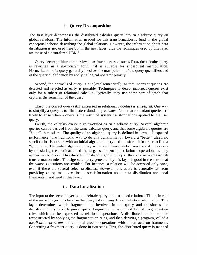
i. Query Decomposition
The first layer decomposes the distributed calculus query into an algebraic query on
global relations. The information needed for this transformation is fund in the global
conceptual schema describing the global relations. However, the information about data
distribution is not used here but in the next layer. thus the techniques used by this layer
are those of a centralized DBMS.
Query decomposition can be viewed as four successive steps. First, the calculus query
is rewritten in a normalized form that is suitable for subsequent manipulation.
Normalization of a query generally involves the manipulation of the query quantifiers and
of the query qualification by applying logical operator priority.
Second, the normalized query is analyzed semantically so that incorrect queries are
detected and rejected as early as possible. Techniques to detect incorrect queries exist
only for a subset of relational calculus. Typically, they use some sort of graph that
captures the semantics of the query.
Third, the correct query (still expressed in relational calculus) is simplified. One way
to simplify a query is to eliminate redundant predicates. Note that redundant queries are
likely to arise when a query is the result of system transformations applied to the user
query.
Fourth, the calculus query is restructured as an algebraic query. Several algebraic
queries can be derived from the same calculus query, and that some algebraic queries are
“better” than others. The quality of an algebraic query is defined in terms of expected
performance. The traditional way to do this transformation toward a “better” algebraic
specification is to start with an initial algebraic query and transform it in order to find a
“good” one. The initial algebraic query is derived immediately from the calculus query
by translating the predicates and the target statement into relational operations as they
appear in the query. This directly translated algebra query is then restructured through
transformation rules. The algebraic query generated by this layer is good in the sense that
the worse executions are avoided. For instance, a relation will be accessed only once,
even if there are several select predicates. However, this query is generally far from
providing an optimal execution, since information about data distribution and local
fragments is not used at this layer.
ii. Data Localization
The input to the second layer is an algebraic query on distributed relations. The main role
of the second layer is to localize the query’s data using data distribution information. This
layer determines which fragments are involved in the query and transforms the
distributed query into a fragment query. Fragmentation is defined through fragmentation
rules which can be expressed as relational operations. A distributed relation can be
reconstructed by applying the fragmentation rules, and then deriving a program, called a
localization program, of relational algebra operations which then acts on fragments.
Generating a fragment query is done in two steps. First, the distributed query is mapped

into a fragment query by substituting each distributed relation by its reconstruction
program (also called materialization program), Second, the fragment query is simplified
and restructured to produce another “good” query. Simplification and restructuring may
be done according to the same rules used in the decomposition layer. As in the
decomposition layer, the final fragment query is generally far from optimal because
information regarding fragments is not utilized.
iii. Global Query Optimization
The input to the third layer is a fragment query, that is, an algebraic query on fragments.
The goal of query optimization is to find an execution strategy for the query which is
close to optimal. Remember that finding the optimal solution is computationally
intractable. An execution strategy for a distributed query can be described with relational
algebra operations and communication primitives (send/receive operations) for
transferring data between sites. The previous layers have already optimized the query, for
example, by eliminating redundant expressions. However, this optimization is
independent of fragment characteristics such as cardinalities. In addition, communication
operations are not yet specified by permuting the ordering of operations within one
fragment query, many equivalent queries may be found.
Query optimization consists of finding the “best” ordering of operations in the fragment
query, including communication operations which minimize a cost function. The cost
function, often defined in terms of time units, refers to computing resources such as disk
space, disk I/Os, buffer space, CPU cost, communication cost, and so on. Generally, it is
a weighted combination of I/O, CPU, and communication costs. Nevertheless, a typical
simplification made by distributed DBMSs, as we mentioned before, is to consider
communication cost as the most significant factor. This is valid for wide area networks,
where the limited bandwidth makes communication much more costly than local
processing. To select the ordering of operations it is necessary to predict execution costs
of alternative candidate orderings. Determining execution costs before query execution
(i.e., static optimization) is based on fragment statistics and the formulas for estimating
the cardinalities of results of relational operations. Thus the optimization decisions
depend on the available statistics on fragments.
An important aspect of query optimization is join ordering, since permutations of the
joins within the query may lead to improvements of orders of magnitude.
One basic technique for optimizing a sequence of distributed join operations is
through the semijoin operator. The main value of the semijoin in a distributed system is
to reduce the size of the join operands and then the communication cost. However, more
recent techniques, which consider local processing costs as well as communication costs,
do not use semijoins because they might increase local processing costs. The output of
the query optimization layer is an optimized algebraic query with communication
operations included on fragments.
iv. Local Query Optimization

The last layer is performed by all the sites having fragments involved in the query. Each
subquery executing at one site, called a local query, is then optimized using the local
schema of the site. At this time, the algorithms to perform the relational operations may
be chosen. Local optimization uses the algorithms of centralized systems.
2. Explain query decomposition steps in details.
v. Query Decomposition
The first layer decomposes the distributed calculus query into an algebraic query on
global relations. The information needed for this transformation is fund in the global
conceptual schema describing the global relations. However, the information about data
distribution is not used here but in the next layer. thus the techniques used by this layer
are those of a centralized DBMS.
Query decomposition can be viewed as four successive steps. First, the calculus query
is rewritten in a normalized form that is suitable for subsequent manipulation.
Normalization of a query generally involves the manipulation of the query quantifiers and
of the query qualification by applying logical operator priority.
Second, the normalized query is analyzed semantically so that incorrect queries are
detected and rejected as early as possible. Techniques to detect incorrect queries exist
only for a subset of relational calculus. Typically, they use some sort of graph that
captures the semantics of the query.
Third, the correct query (still expressed in relational calculus) is simplified. One way
to simplify a query is to eliminate redundant predicates. Note that redundant queries are
likely to arise when a query is the result of system transformations applied to the user
query. As seen in Chapter 6, such transformations are used for performing semantic data
control (views, protection, and semantic integrity control).
Fourth, the calculus query is restructured as an algebraic query. several algebraic
queries can be derived from the same calculus query, and that some algebraic queries are
“better” than others. The quality of an algebraic query is defined in terms of expected
performance. The traditional way to do this transformation toward a “better” algebraic
specification is to start with an initial algebraic query and transform it in order to find a
“good” one. The initial algebraic query is derived immediately from the calculus query
by translating the predicates and the target statement into relational operations as they
appear in the query. This directly translated algebra query is then restructured through
transformation rules. The algebraic query generated by this layer is good in the sense that
the worse executions are avoided. For instance, a relation will be accessed only once,
even if there are several select predicates. However, this query is generally far from
providing an optimal execution, since information about data distribution and local
fragments is not used at this layer.

3. What is the Complexity of Relational Algebra Operation?
COMPLEXITY OF RELATIONAL ALGEBRA OPERATIONS
In this chapter we consider relational algebra as a basis to express the output of query
processing. Therefore, the complexity of relational algebra operations, which directly
affects their execution time, dictates some principles useful to a query processor. These
principles can help in choosing the final execution strategy.
The simplest way of defining complexity is in terms of relation cardinalities
independent of physical implementation details such as fragmentation and storage
structures. complexity of unary and binary operations in the order of increasing
complexity, and thus of increasing execution time. Complexity is O(n) for unary
operations, where n denotes the relation cardinality, if the resulting tuples may be
obtained independently of each other. Complexity is O(n * logn) for binary operation if
each tuple of one relation must be compared with each tuple of the other on the basis of
the equality of selected attributes. This complexity assumes that tuples of each relation
must be sorted on the comparison attributes. Projects with duplicate elimination and
group operations require O(n * logn) complexity. Finally, complexity is O(n2) for the
Cartesian product of two relations because each tuple of one relation must be combined
with each tuple of the other.
This simple look at operation complexity suggests two principles. First, because
complexity is relative to relation cardinalities, the most selective operations that reduce
cardinalities (e.g., selection) should be performed first. Second, operations should be
ordered by increasing complexity so that Cartesian products can be avoided or delayed.
4. What are the characteristic that are applicable only for
distributed Query processor?
1. CHARACTERIZATION OF QUERY PROCESSORS
It is quite difficult to evaluate and compare query processors in the context of both
centralized systems and distributed systems because they may differ in many aspects. In
what follows, we list important characteristics of query processors that can be used as a
basis for comparison. The first four characteristics hold for both centralized and
distributed query processors, while the next four characteristics are particular to
distributed query processors.
2. Languages

Initially, most work on query processing was done in the context of relational DBMSs
because their high-level languages give the system many opportunities for optimization.
The input language to the query processor can be based on relational calculus or
relational algebra. With object DBMSs, the language is based on object calculus which is
merely an extension of relational calculus. Thus, decomposition in object algebra is also
needed.
The former requires an additional phase to decompose a query expressed in relational
calculus into relational algebra. In a distributed context, the output language is generally
some internal form of relational algebra augmented with communication primitives. The
operations of the output language are implemented directly in the system. Query
processing must perform efficient mapping form the input language to the output
language.
3. Types of Optimization
Conceptually, query optimization aims at choosing the best point in the solution space of
all possible execution strategies. An immediate method for query optimization is to
search the solution space, exhaustively predict the cost of each strategy, and select the
strategy with minimum cost. Although this method is effective in selecting the best
strategy, it may incur a significant processing cost for the optimization itself. The
problem is that the solution space can be large; that is, there may be many equivalent
strategies, even with a small number of relations. The problem becomes worse as the
number of relations or fragments increases Having high optimization cost is not
necessarily bad, particularly if query optimization is done once for many subsequent
executions of the query. Therefore, an “exhaustive” search approach is often used
whereby (almost) all possible execution strategies are considered.
To avoid the high cost of exhaustive search, randomized strategies, such as Iterative
Improvement have been proposed. They try to find a very good solution, not necessarily
the best one, but avoid the high cost of optimization, in terms of memory and time
consumption.
Another popular way of reducing the cost of exhaustive search is the use of heuristics,
whose effect is to restrict the solution space so that only a few strategies are considered.
In both centralized and distributed systems, a common heuristic is to minimize the size of
intermediate relations. This can be done by performing unary operations first, and
ordering the binary operations by the increasing sizes of their intermediate relations. An
important heuristic in distributed systems is to replace join operations by combinations of
semijoins to minimize data communication.
4. Optimization Timing
A query may be optimized at different times relative to the actual time of query
execution. Optimization can be done statically before executing the query r dynamically
as the query is executed. Static query optimization is done at query compilation time.

Thus the cost of optimization may be amortized over multiple query executions.
Therefore, this timing is appropriate for use with the exhaustive search method. Since the
sizes of the intermediate relations of a strategy are not known until run time, they must be
estimated using database statistics. Errors in these estimates can lead to the choice of
suboptimal strategies.
Dynamic query optimization proceeds at query execution time. At any point of
execution, the choice of the best next operation can be based on accurate knowledge of
the results of the operations executed previously. Therefore, database statistics are not
needed to estimate the size of intermediate results. However, they may still be useful in
choosing the first operations. The main advantage over static query optimization is that
the actual sizes of intermediate relations are available to the query processor, thereby
minimizing the probability of a bad choice. The main shortcoming is that query
optimization, an expensive task, must be repeated for each execution of the query.
Therefore, this approach is best for ad-hoc queries.
Hybrid query optimization attempts to provide the advantages of static query
optimization while avoiding the issues generated by inaccurate estimates. The approach is
basically static, but dynamic query optimization may take place at run time when a high
difference between predicted sizes and actual size of intermediate relations is detected.
5. Statistics
The effectiveness of query optimization relies on statistics on the database. Dynamic
query optimization requires statistics in order to choose which operations should be done
first. Static query optimization is even more demanding since the size of intermediate
relations must also be estimated based on statistical information. In a distributed
database, statistics for query optimization typically bear on fragments, and include
fragment cardinality and size as well as the size and number of distinct values of each
attribute. To minimize the probability of error, more detailed statistics such as histograms
of attribute values are sometimes used at the expense of higher management cost. The
accuracy of statistics is achieved by periodic updating. With static optimization,
significant changes in statistics used to optimize a query might result in query
reoptimizaion.
6. Decision Sites
When static optimization is used, either a single site or several sites may participate in the
selection of the strategy to be applied for answering the query. Most systems use the
centralized decision approach, in which a single site generates the strategy. However, the
decision process could be distributed among various sites participating in the elaboration
of the best strategy. The centralized approach is simpler but requires knowledge of the
entire distributed database, while the distributed approach requires only local
information. Hybrid approaches where one site makes the major decisions and other sites
can make local decisions are also frequent.

7. Exploitation of the Network Topology
The network topology is generally exploited by the distributed query processor. With
wide area networks, the cost function to be minimized can be restricted to the data
communication cost, which is considered to be the dominant factor. This assumption
greatly simplifies distributed query optimization, which can be divided into two separate
problems: selection of the global execution strategy, based on intersite communication,
and selection of each local execution strategy, based on a centralized query processing
algorithm.
With local area networks, communication costs are comparable to I/O costs.
Therefore, it is reasonable for the distributed query processor to increase parallel
execution at the expense of communication cost. The broadcasting capability of some
local area networks can be exploited successfully to optimize the processing of join
operations .Other algorithms specialized to take advantage of the network topology are
presented in for star networks and in for satellite networks.
In a client-server environment, the power of the client workstation can be exploited to
perform database operations using data shipping. The optimization problem becomes to
decide which part of the query should be performed on the client and which part on the
server using query shipping.
8. Exploitation of Replicated Fragments
Distributed queries expressed on global relations are mapped into queries on physical
fragments of relations by translating relations into fragments. We call this process
localization because its main function is to localize the data involved in the query. For
reliability purposes it is useful to have fragments replicated at different sites. Most
optimization algorithms consider the localization process independently of optimization.
However, some algorithms exploit the existence of replicated fragments at run time in
order to minimize communication times. The Optimization algorithm is then more
complex because there are a larger number of possible strategies.
9. Use of Semijoins
The semijoin operation has the important property of reducing the size of the operand
relation. When the main cost component considered by the query processor is
communication, a semijoin is particularly useful for improving the processing of
distributed join operations as it reduces the size of data exchanged between sites.
However, using semijoins may result in an increase in the number of messages and in the
local processing time. The early distributed DBMSs, such as SDD-, which wee designed
for slow wide area networks, make extensive use of semijoins. Some later systems, such
as R* ,assume faster networks and do not employ semijoins. Rather, they perform
semijoins are still beneficial in the context of fast networks when they induce a
algorithms aim at selecting an optimal combination of joins and semijoins.
Unit IV
1. Explain traction management in details.
The fundamental point here is that there is no notion of “consistent execution” or
“reliable computation” associated with the concept of a query. The concept of a
transaction is used within the database domain as a basic unit of consistent and reliable
computing. Thus queries are executed as transactions once their execution strategies are
determined and they are translated into primitive database operations.
In the discussion above, we used the terms consistent and reliable quite informally.
Due to their importance in our discussion, we need to define them more precisely. We
should first point out that we differentiate between database consistency and transaction
consistency.
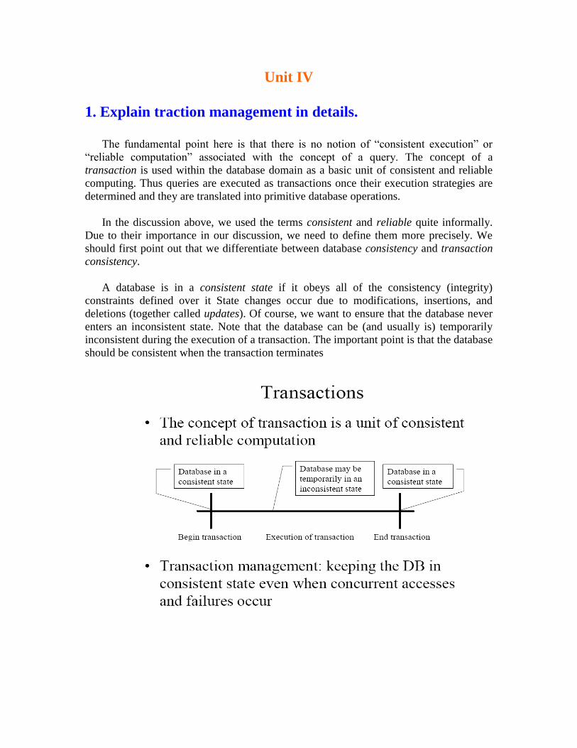
A database is in a consistent state if it obeys all of the consistency (integrity)
constraints defined over it State changes occur due to modifications, insertions, and
deletions (together called updates). Of course, we want to ensure that the database never
enters an inconsistent state. Note that the database can be (and usually is) temporarily
inconsistent during the execution of a transaction. The important point is that the database
should be consistent when the transaction terminates

Transaction consistency, on the other hand, refers to the actions of concurrent
transactions. We would like the database to remain in a consistent state even i9f there are
a number of user requests that are concurrently accessing (reading or updating) the
database. A complication arises when replicated databases are considered. A replicated
database is in a mutually consistent state if all the copies of every data item in it have
identical values. This is referred to as one-copy equivalence since all replica copies are
forced to assume the same state at the end of a transaction’s execution. There are more
relaxed notions of replica consistency that allow replica values to diverge. These will be
discussed later in the text.
Reliability refers to both the resiliency of a system to various types of failures and its
capability to recover from them. A resilient system is tolerant of system failures and can
continue to provide services even when failures occur. A recoverable DBMS is one that
can get to a consistent state (by moving back to a previous consistent state or forward to a
new consistent state) following various types of failures.
Transaction management deals with the problems of always keeping the database in a
consistent state even when concurrent accesses and failures occur. In the upcoming two
chapters, we investigate the issues related to managing transactions. The purpose of the
current chapter is to define the fundamental terms and to provide the framework within
which these issues can be discussed. It also serves as a concise introduction to the
problem and the related issues. We will therefore discuss the concepts at a high level of
abstraction and will not present any management techniques.
DEFINITION OF A TRANSACTION
The transaction concept has its roots in contract law. states, “In making a contract, two or
more parties negotiate for a while and then make a deal. The deal is made binding by the
joint signature of a document or by some other act (as simple as a handshake or a nod). If
the parties are rather suspicious of one another or just want to be safe, they appoint an
intermediary (usually called an escrow officer) to coordinate the commitment of the
transaction. “The nice aspect of this historical perspective is that the description above
does indeed encompass some of the fundamental properties of a transaction (atomicity
and durability) as the term is used in database systems. It also serves to indicate the
differences between a transaction and a query.
As indicated before, a transaction is a unit of consistent and reliable computation.
Thus, intuitively, a transaction takes a database, performs an action on it, and generates a
new version of the database, causing a state transition. This is similar to what a query
does, except that if the database was consistent before the execution of the transaction,
we can now guarantee that it will be consistent at the end of its execution regardless of
the fact that (1) the transaction may have been executed concurrently with others, and (2)
failures may have occurred during its execution.
In general, a transaction is considered to be made up of a sequence of read and write
operations on the database, together with computation steps. In that sense, a transaction
may be thought of as a program with embedded database access queries. Another
definition of a transaction is that it is a single execution of a program. A single query can
also be thought of as a program that can be posed as a transaction.
2. Explain how to formalize a transaction with example.
Formalization of the Transaction Concept
By now, the meaning of a transaction should be intuitively clear. To reason about
transactions and about the correctness of the management algorithms, it is necessary to
define the concept formally. We denote by Oij(x) some operation Oj of transaction Ti that
operates on a database entity x. following the conventions adopted in the preceding
section, Oij {read, write}. Operations are assumed to be atomic (i.e., OSi = j Oij). We
denote by Ni the termination condition for Ti, where Ni{abort, commit}.2
With this terminology we can define a transaction Ti as a partial ordering over its
operations and the termination condition. A partial order P = { , }defines an ordering
among the elements of (called the domain) according to an irreflexive and transitive
binary relation defined over . in our case consists of the operations and termination
condition of a transaction, whereas indicates the execution order of these operations
(which we will read as “precedes in execution order”). Formally, then, a transaction Ti is
a partial order Ti = { i, j }, where
1. i = OSi {Ni}.
2. For an two operations Oij, Oik, OSi, if Oij = {R(x) or W(x)} and Ojk = W(x)
for any data item x, then either Oij i Oik or Oik Oij.
3. Oij OSi, Oij i Ni.
The first condition formally defines the domain as the set of read and write operations
that make up the transaction, plus the termination condition, which may be either commit
or abort. The second condition specifies the ordering relation between the conflicting
read and write operations of the transaction, while the final condition indicates that the
termination condition always follows all other operations.
There are two important points about this definition. First, the ordering relation is
given and the definition does not attempt to construct it. The ordering relation is actually
application dependent. Second, condition two indicates that the ordering between
conflicting operations has to exist within . Two operations, Oi(x) and Oj(x), are said to
be in conflict if Oi = Write or Oj = Write (i.e., at least one of them is a Write and they
access the same data item).
Example
Consider a simple transaction T that consists of the following steps:

Read(x)
Read(y)
x← x + y
Write(x)
Commit
The specification of this transaction according to the formal notation that we have
introduced is as follows:
= {R(x), R(y), W(x), C}
= {(R(x), W(x)), R(y), W(x), W(x), (CT), (R(x), C), (R(y)tC)}
Where (Oi, Oj) as an element of the relation indicates that Oi Oj.
Notice that ordering relation specifies the relative ordering of all operations with respect
to the termination condition. This is due to the third condition of ransaction definition.
Also note that we do not specify the ordering between every pair of operations. That is
why it is a partial order.
3. Explain the following terms-
i. cascading aborts.
ii. Degree of consistency
iii. Transaction recovery
iv. Types of workflows.
i. cascading aborts obviously, the fact that if no free seats are available, the transaction is aborted.1 The
second is the ordering of the output to the user with respect to the abort and commit
commands. Note that if the transaction is aborted, the user can be notified before the
DBMS is instructed to abort it. However, in case of commit, the user notification has to
follow the successful servicing (by the DBMS) of the commit command, for reliability
reasons ii Consistency
The consistency of a transaction is simply its correctness. In other words, a transaction is
a correct program that maps one consistent database state to another. Verifying that
transactions are consistent is the concern of semantic data control, covered in Chapter 6.
ensuring transaction consistency as defined at the beginning of this chapter, on the other
hand, is the objective of concurrency control mechanisms, which we discuss in Chapter
11.
There is an interesting classification consistency that parallels our discussion above
and is equally important. This classification groups database into four levels of
consistency [Gray et al., 1976]. In the following definition (which is taken verbatim from
the original paper), dirty data refers to data values that have been updated by a transaction
prior to its commitment. Then, based on the concept of dirty data, the four levels are
defined as follows:
“Degree 3: Transaction T sees degree 3 consistency if:
1. T does not overwrite dirty data of other transactions.
2. T does not commit any writes until it completes all its writes [i.e., until the end of
transaction (EOT)].
3. T does not read dirty data from other transactions.
4. Other transactions do to dirty any data read by T before T completes.
Degree 2: Transaction T sees degree 2 consistency if:
1. T does not overwrite dirty data of other transactions.
2. T does not commit any writes before EOT.
3. T does not read dirty data from other transactions.
Degree 1: Transaction T sees degree 1 consistency if:
1. T does not overwrite dirty data of other transactions.
2. T does not commit any writes before EOT.
Degree 0: Transaction T sees Degree 0 consistency if:
1. T does not overwrite dirty data of other transactions.”
Of course, it is true that a higher degree of consistency encompasses all the lower
degrees. The point in defining multiple levels of consistency is to provide application
programmers the flexibility to define transactions that operate at different levels.
Consequently, while some transactions operate at Degree 3 consistency level, other may
operate at lower levels and may see, for example, dirty data.
iii. Transaction recovery One can generally talk about two types of failures. A transaction itself may fail due
to input data errors, deadlocks, or other factors. In these cases either the transaction
aborts itself, as we have seen in Example 10.2, or the DBMS may abort it while handling
deadlocks, for example. Maintaining transaction atomicity in the presence of this type of
failure is commonly called the transaction recovery. The second type of failure is caused
by system crashes, such as media failures, processor failures, communication link
breakages, power outages, and so on. Ensuring transaction atomicity in the presence of
system crashes is called crash recovery.
Iv three types of workflows are identified:
1. Human-oriented workflows, which involve humans in performing the tasks. The
system support is provided to facilitate collaboration and coordination among
humans, but it is the humans themselves who are ultimately responsible for the
consistency of the actions.
2. System-oriented workflows are those which consist of computation-intensive and
specialized tasks that can be executed by a computer. The system support in this
case is substantial and involves concurrency control and recovery, automatic task
execution, notification, etc.
3. Transactional workflows range in between human-oriented and system-oriented
workflows and borrow characteristics from both. They involve “coordinated
execution of multiple tasks that (a) may involve humans, (b) require access to
HAD [heterogeneous, autonomous, and/or distributed] systems, and (c) support
selective use of transactional properties [i.e., ACID properties] for individual
tasks or entire workflows.” [Georgakopoulos et al., 1995].
4. Comment on “workflows are better than flat and nested
transaction” Nested Transactions
An alternative transaction model is to permit a transaction to include other transactions
with their own begin and commit points. Such transactions are called nested transactions.
These transactions that are embedded in another one are usually called subtransactions.
Example
Let us extend the reservation transaction of Example. Most travel agents will make
reservations for hotels and car rentals in addition to the flights. If one chooses to
specify all of this as one transaction, the reservation transaction would have the
following structure:
Begin_transaction Reservation
begin Begin_transaction Airline
…
end. {Airline}
Begin_transaction Hotel
…
end. { Hotel }
Begin_transaction Car
…
end. { Car }
end.
Nested transactions have received considerable interest as a more generalized
transaction concept. The level of nesting is generally open, allowing subtransactions
themselves to have nested transactions. This generality is necessary to support application
areas where transactions are more complex than in traditional data processing.
In this taxonomy, we differentiate between closed and open nesting because of their
termination characteristics. Closed nested transactions commit in a bottom-up fashion
through the root. Thus, a nested subtransaction begins after its parent and finishes before
it, and the commitment of the subtransactions is conditional upon the commi8tment of the
parent. The semantics of these transaction enforce atomicity at the top-most level. Open
nesting relaxes the top-level atomicity restriction of closed nested transactions. Therefore,
an open nested transaction allows its partial results to be observed outside the transaction.
Sagas and split transactions are examples of open nesting.
A saga is a “sequence of transactions that can be interleaved with other transactions”
are run to recover from a partial execution. A compensating transaction effectively does
the inverse of the transaction that it is associated with. For example, if the transaction
adds $100 to a bank account, its compensating transaction deducts $100 from the same
bank account. If a transaction is viewed as a function, f, that maps the old database state
to a new database state, its compensating transaction is the inverse function, f’.
Two properties of sagas are: (1) only two levels of nesting are allowed, and (2) at the
outer level, the system does not support full atomicity. Therefore, a saga differs from a
closed nested transaction in that its level structure is more restricted (only 2) and that it is
open (the partial results of component transactions or sub-sagas are visible to the
outside). Furthermore, the transactions that make up a saga have to be executed
sequentially.
The saga concept is extended in and placed within a more general model that deals
with long-lived transactions and with activities which consist of multiple steps. The
fundamental concept of the model is that of a module which captures code segments that
accomplish a given task and access a database in the process. The modules are modeled
(at some level) as sub-sagas which communicate with each other via messages over ports.
The transactions that make up a saga can be executed in parallel. The model is multi-
layer where each subsequent layer adds a level of abstraction.
The advantages of nested transaction are the following. First, they provide a higher-
level of concurrency among transactions. Since a transaction consists of a number of
other transactions, more concurrency is possible within a single transaction. For example,
if the reservation transaction of Example is implemented as a flat transaction, it may not
be possible to access records about specific flight concurrently. In other words, if one
travel agent issues the reservation transaction for a given flight, any concurrent
transaction that wishes to access same flight data will have to wait until the termination
of the first, which includes the hotel and car reservation activities in addition to flight

reservation. However, a nested implementation will permit the second transaction to
access the flight data as soon as the Airline subtransaction of the first reservation
transaction is completed. In other words, it may be possible to perform a finer level of
synchronization among concurrent transactions.
A second argument in favor of nested transaction is related to recovery. It is possible
to recover independently from failures of each subtransaction. This limits the damage to a
smaller part of the transaction, making it less costly to recover. In a flat transaction, if any
operation fails, the entire transaction has to be aborted and restarted, whereas in a nested
transaction, if an operation fails, only the subtransaction containing that operation needs
to be aborted and restarted.
Finally, it is possible to create new transactions from existing ones simply by
inserting the old one inside the new one as a subtransaction.
Workflows
Flat transactions model relatively simple and short activities very well. However, they are
less appropriate for modeling longer and more elaborate activities. That is the reason for
the development of the various nested transaction models discussed above. It has been
argued that these extensions are not sufficiently powerful to model business activities:
“after several d3ecades of data processing, we have learned that we have not won the
battle of modeling and automating complex enterprises” To meet these needs, more
complex transaction models which are combinations of open and nested transactions have
been proposed. There are well-justified arguments for not calling these transactions, since
they hardly follow any of the ACID properties; a more appropriate name that has been
proposed is a workflow
The term “workflow,” unfortunately, does not have a clear and uniformly accepted
meaning. A working definition is that a workflow is “a collection of tasks organized to
accomplish some business process.” This definition, however, leaves a lot undefined.
This is perhaps unavoidable given the very different contexts where this term is used. In
three types of workflows are identified:
4. Human-oriented workflows, which involve humans in performing the tasks. The
system support is provided to facilitate collaboration and coordination among
humans, but it is the humans themselves who are ultimately responsible for the
consistency of the actions.
5. System-oriented workflows are those which consist of computation-intensive and
specialized tasks that can be executed by a computer. The system support in this
case is substantial and involves concurrency control and recovery, automatic task
execution, notification, etc.
6. Transactional workflows range in between human-oriented and system-oriented
workflows and borrow characteristics from both. They involve “coordinated
execution of multiple tasks that (a) may involve humans, (b) require access to
HAD [heterogeneous, autonomous, and/or distributed] systems, and (c) support
selective use of transactional properties [i.e., ACID properties] for individual
tasks or entire workflows.”
Among the features of transactional workflows, the selective use of transactional
properties is particularly important as it characterizes possible relaxations of
ACID properties.
In this book, our primary interest is with transactional workflows. There have been
many transactional workflow proposals which differ in a number of ways. The common
point among them is that a workflow is defined as an activity consisting of a set of tasks
with well-defined precedence relationship among them.
Example
Let us further extend the reservation transaction of Example. The entire reservation
activity consists of the following taks and involves the following data.
Customer request is obtained (task T1) and Customer Database is accessed to
obtain customer information, preferences, etc.;
Airline reservation is performed (T2) by accessing the Flight Database;
Hotel reservation is performed (T3), which may involve sending a message to the
hotel involved;
Auto reservation is performed (T4), which may also involve communication with
the car rental company;
Bill is generated (T5) and the billing info is recorded in the billing database.
Figure depicts this workflow where there is a serial dependency of T2 on T1, and T3,
T4 on T2; however, T3 and T4 (hotel and car reservations) are performed in parallel
and T5 waits until their completion.
A number of workflow model go beyond this basic model by both defining more
precisely what tasks can be and by allocating different relationships among the tasks. In
the following, we define one model which is similar to the models.A workflow is
modeled as an activity which has open nesting semantics in that it permits partial results
to be visible outside the activity boundaries. Thus, tasks which make up the activity are
allowed to commit individually. Tasks may be other activities (with the same open
transaction semantics) or closed nested transactions that make their results visible to the
entire system when they commit. Even though an activity can have both other activities
and closed nested transactions as its component, a closed nested transaction task can only
be composed of other closed nested transactions (i.e., once closed nesting semantics
begins, it is maintained for all components).

An activity commits when its components are read to commit. However, the
components commit individually, without waiting for the root activity to commit. This
raises problems in dealing with aborts since when an activity aborts, all of its components
should be aborted. The problem is dealing with the components that have already
committed. Therefore, compensating transactions are defined for the components of an
activity. Thus, if a component has already committed when and activity aborts, the
corresponding compensating transaction is executed to “undo” its effects.
Some components of an activity may be marked as vital. When a vital component
aborts, its parent must also abort. If a non-vital component of a workflow model aborts, it
may continue executing. A workflow, on the other hand, always aborts when one of its
components aborts. For example, in the reservation workflow of T1 (airline reservation)
and T2 (hotel reservation) may be declared as vital so that if an airline reservation or a
hotel reservation cannot be made, the workflow aborts and the entire trip is canceled.
However, if a car reservation cannot be committed, the workflow can still successfully
terminate.
It is possible to define contingency tasks which are invoked if their counter-parts fail.
For example, in the Reservation example presented earlier, one can specify that the
contingency to making a reservation at Hilton is to make a reservation Sheraton. Thus, if
the hotel reservation component for Hilton falls, the Sheraton alternative is tired rather
than aborting the task and the entire workflow.
Unit V
1. Discuss the seriazalibility theory in concurrency control. SERIALIZABILITY THEORY
the concurrent execution of transactions leaves the database in a state that can be
achieved by their serial execution in some order, problems such as lost updates will be
resolved. This is exactly the point of the serializability argument. The remainder of this
section addresses serializability issues more formally.
A schedule S (also called a history) is defined over a set of transactions T
= {T1, T2, … , Tn} and specifies an interleaved order of execution of these transactions’
operations. Based on the definition of a transaction introduced in Section 10.1, the
schedule can be specified as a partial order over T. We need a few preliminaries, though,
before we present the formal definition.
Recall the definition of conflicting operations that we gave in Chapter 10. Two
operations Oij(x) and Okl(x) (i and k not necessarily distinct) accessing the same database
entity x are said to be in conflict if at least one of them is a write. Note two things in this
definition. First, read operations do not conflict with each other. We can, therefore, talk
about two types of conflicts: read-write (or write-read), and write-write. Second, the two

operations can belong to the same transaction or to two different transactions. In the latter
case, the two transactions are said to be conflicting. Intuitively, the existence of a conflict
between two operations indicate that their order of execution is important. The ordering
of two read operations is insignificant.
We first define a complete schedule, which defines the execution order of all
operations in its domain. We will then define a schedule as a prefix of a complete
schedule. Formally, a complete schedule c
TS defined over a set of transactions T
= {T1, T2, … , Tn} is a partial order c
TS = {T ,
T }where
1. i
n
iT 1 .
2. i
n
iT 1 .
3. For any two conflicting operations Oij, Okl T , > either Oij, T Okl, or
Okl, T Oij.
The first condition simply states that the domain of the schedule is the union of the
domains of individual transactions. The second condition defines the ordering relation as
a superset of the ordering relations of individual transaction. This maintains the ordering
of operations within each transaction. The final condition simply defines the execution
order among conflicting operations.
Example
Consider the two transactions from Example 10.8. They were specified as
T1: Read(x) T2: Read(x)
x ← x + 1 x ← x + 1
Write(x) Write(x)
Commit Commit
A possible complete schedule c
TS over T = { T1, T2} can be written as the following
partial order (where the subscripts indicate the transactions):
c
TS = {T ,
T }
where
1 = {R1(x), W1(x), C1}
2 = {R2(x), W2(x), C2}
Thus
T = 1
2 = {R1(x), W1(x), C1, R2(x), W2(x)}

and
T = {(R1, R2), (R1, W1), (R1, C1), (R1, W2), (R1, C2), (R2, W1),
(R2, C1), (R2, W2), (R2, C2), (W1, C1), (W1, W2), (W1, C2),
(C1, W2), (C1, C2), (W2, C2)}
2. Explain nested distributed transaction
Nested Distributed Transactions
We introduced the nested transaction model in the previous chapter. The concurrent
execution of nested transactions is interesting, especially since they are good candidates
for distributed execution.
The concurrency control of nested transactions have generally followed a locking-
based approach. The following rules govern the management of the locks and the
completion of transaction execution in the case of closed nested transactions:
1. Each subtransaction executes as a transaction and upon completion transfers its
lock to its parent transaction.
2. A parent inherits both the locks and the updates of its committed sub-transactions.
3. the inherited state will be visible only to descendants of the inheriting parent
transaction. However, to access the sate, a descendant must acquire appropriate
locks. Lock conflicts are determined as for flat transactions, except that one
ignores inherited locks retained by ancestor’s of the requesting subtransaction.
4. If a subtransaction aborts, then all locks and updates that the subtransaction and
its descendants are discarded. The parent of an aborted subtransaction need not,
but may, choose to abort.
Prom the perspective of ACID properties, closed nested transactions relax durability
since the effects of successfully completed subtransactions can be erased if an ancestor
transaction aborts. They also relax the isolation property in a limited way since they share
their state with other subtransactions within the same nested transaction.
The distributed execution potential of nested transactions is obvious. After all, nested
transactions are meant to improve intra-transaction concurrency and one can view each
subtransaction as a potential unit of distribution if data are also appropriately distributed.
However, from the perspective of lock management, some care has to be observe.
When subtransactions release their locks to their parents, these lock releases cannot be
reflected in the lock tables automatically. Open nested transactions are even more relaxed
than their closed nested counterparts. They have been called ‘anarchic” forms of nested
transactions The open nested transaction model is best exemplified in the saga model

From the perspective of lock management, open nested transactions are easy to deal
with. The locks held by a subtransaction are released as soon as it commits or aborts and
this is reflected in the lock tables.
Consider two transactions that transfer funds from one bank account to another:
T1: Withdraw(o, x) T2: Withdraw(o, y)
Deposit(p, x) Deposit(p, y)
The notation here is that each Ti withdraws x amount from account o and deposits that
amount to account p. the semantics of Withdraw is test-and-with-draw to ensure that the
account balance is sufficient to meet the withdrawal request. In relational systems, each
of these abstract operations will be translated to tuple operations Select (Sel), and Update
(Upd) which will, in turn, be translated into page-level Read and Write operations.
2. Explain optimistic concurrency control algorithm
OPTIMISTIC CONCURRENCY CONTROL ALGORITHMS
the conflicts between transactions are quite frequent and do not permit a transaction to
access a data item if there is a conflicting transaction that accesses that data item. Thus
the execution of any operation of a transaction follows the sequence of phases: validation
Generally, this sequence is valid for an update transaction as well as for each of its
operations.
an operation submitted to an optimistic scheduler is never delayed. The read,
compute, and write operations of each transaction are processed freely without updating
the actual database. Each transaction initially makes its updates on local copies of data
items. The validation phase consists of checking if these updates would maintain the
consistency of the database. If the answer is affirmative, the changes are made global
(i.e., written into the actual database). Otherwise, the transaction is aborted and has to
restart.
only the optimistic approach using timestamps. Our discussion is brief and
emphasizes concepts rather than implementation details. The reasons for this are twofold.
First, most of the current work on optimistic methods concentrates on centralized rather
than distributed DBMSs. Second, optimistic algorithms have not been implemented in
any commercial or prototype DBMS. Therefore, the information regarding their
implementation trade-offs is insufficient. As a matter of fact, the only centralized
implementation of optimistic concepts (not the full algorithm) is in IBM’s IMS-
FASTPATH, which provides primitives that permit the programmer to access the
database in an optimistic manner.

It differs from pessimistic TO-based algorithms not only by being optimistic byt also
in its assignment of timestamps. Timestamps are associated only with transactions, not
with data items (i.e., there are no read or write timestamps). Furthermore, timestamps are
not assigned to transaction at their initiation but at the beginning of their validation step.
This is because the timestamps are needed only during the validation phase, and as we
will see shortly, their early assignment may cause unnecessary transaction rejections.
Each transaction Tj is subdivided (by the transaction manager at the originating site)
into a number of subtransactions, each of which can execute at many sites. Notationally,
let us denote by Tij a subtransaction of Ti that executes at site j. Until the validation phase,
each local execution follows the sequence depicted in Figure 11.13 At that point a
timestamp is assigned to the transaction which is copied to all its subtransactions. The
local validation of Ty is performed according to the following rules, which are mutually
exclusive.
Rule 1. If all transactions Tk where ts(Tk) < ts(Tij) have completed their write phase
before Tij has started its read phase (Figure 11.14a),3 validation succeeds, because
transaction executions are in serial order.
Rule 2. If there is any transaction Tk such that ts(Tk)< ts(Tij) which completes its
write phase while Tij is in its read phase (Figure 11.14b), the validation succeeds if
WS(Tk) RS(Tij) = Ø
Rule 3. If there is any transaction Tk such that ts(Tk) < ts(Tij) which completes its
read phase before Tij completes its read phase (Figure 11.14c), the validation succeeds if
WS (Tk) RS (Tij) = and WS(Tk) WS (Tij) = .
Rule 1 is obvious; it indicates that the transactions are actually executed serially in
their timestamp order. Rule 2 ensures that none of the data items updated by Tk are read
by Tij, and that Tk finishes writing its updates into the database before Tij starts writing.
Thus the updates of Tij will not be overwritten by the updates of Tk. Rule 3 is similar to
Rule 2, but does not require that Tk finish writing before Tij starts writing. It simply
requires that the updates of Tk not affect the read phase or the write phase of Tij.

Once a transaction is locally validated to ensure that he local database consistency is
maintained, it also needs to be globally validated to ensure that the mutual consistency
rule is obeyed. Unfortunately, there is no known optimistic method of doing this. A
transaction is globally validated if all the transaction that precede it in the serialization
order (at that site0 terminate (either by committing or aborting). This is a pessimistic
method since it performs global validation early and delays a transaction. However, it
guarantees that transaction execute in the same order at each site.
An advantage of the optimistic concurrency control algorithms is their potential to
allow a higher level of concurrency. It has been shown [Kung and Robinson, 1981] that
when transaction conflicts are very rare, the optimistic mechanism performs better than
locking. A major problem with optimistic algorithms is the higher storage cost. To
validate a transaction, the optimistic mechanism has to store the read and the write sets of
terminated transaction. Specifically, the read and write sets of terminated transactions
that were in progress when transaction Tij, arrived at site j need to be stored in order to
validate Tij. Obviously, this increases the storage cost.
Another problem is starvation. Consider a situation in which the validation phase of a
long transaction fails. In subsequent trials it is still possible that the validation will fail
repeatedly. Of course, it is possible to solve this problem by permitting the transaction
exclusive access to the database after a specified number of trials. However, this reduces
the level of concurrency to a single transaction the exact “mix” of transactions that would
cause an intolerable level of restarts is an issue that remains to be studied.
4. How can Deadlock be prevention and avoidance? Deadlock prevention methods guarantee that deadlocks cannot occur in the first place.
Thus the transaction manager checks a transaction when it is first initiated and does not
permit it to proceed if it may cause a deadlock. To perform this check, it is required that

all of the data items that will be accessed by a transaction be predeclared. The transaction
manager then permits a transaction to proceed if all the data items that it will access are
available. Otherwise, the transaction is not permitted to proceed. The transaction manager
reserves all the data items that are predeclared by a transaction that it allows to proceed.
conditional upon the availability of free seats. To be safe, the system would thus need to
consider the maximum set of data items, even if they end up not being accessed. This
would certainly reduce concurrency. Furthermore, there is additional overhead in
evaluating whether a transaction can proceed safely. On the other hand, such systems
require no run-time support, which reduces the overhead. It has the additional advantage
that it is not necessary to abort and restart a transaction due to deadlocks. This not only
reduces the overhead but also makes such methods suitable for systems that have no
provisions for undoing processes.
Deadlock Avoidance
Deadlock avoidance schemes either employ concurrency control techniques that will
never result in deadlocks or require that schedulers detect potential deadlock situations in
advance and ensure that they will not occur. We consider both of these cases.
The simplest means of avoiding deadlocks is to order the resources and insist that
each process request access to these resources in that order. This solution was long ago
proposed for operating systems. A revised version has been proposed for database
systems as well [Garcia-Molina, 1979]. Accordingly, the lock units in the distributed
database are ordered and transactions always request locks in that order. This ordering of
lock units may be done either globally or locally at each site. In the latter case, it is also
necessary to order the sites and require that transactions which access data items at
multiple sites request their locks by visiting the sites in the predefined order.
Another alternative is to make use of transaction timestamps to prioritize transactions
and resolve deadlocks by aborting transactions with higher (or lower) priorities. To
implement this type of prevention method the lock manager is modified as follows. If a
lock request of a transaction Ti is denied, the lock manager does not automatically force
Ti to wait. Instead, it applies a prevention test to the requesting transaction and the
transaction that currently holds the lock (say Tj). If the test is passed, it is permitted to
wait for Tj, otherwise, one transaction or the other is aborted.
WAIT-DIE Rule. If Ti requests a lock on a data item that is already locked by Tj, Tj
is permitted to wait if and only if Ti is older than Tj. If Ti is younger than Tj, then Ti is
aborted and restarted with the same timestamp.
A preemptive version of the same idea is the WOUND-WAIT algorithm, which
follows the rule:

WOUND-WAIT Rule. If Ti requests a lock on a data item that is already locked by
Tj, then Ti is permitted to wait if only if it is younger than Tj, otherwise, Tj is aborted
and the lock is granted to Tj.
The rules are specified from the viewpoint of Ti: Ti waits, Tidies, and Ti wounds Tj. In
fact, the result of wounding and dying are the same: the affected transaction is aborted
and restarted. With this perspective, the two rules can be specified as follows:
if ts(Ti) < ts(Tj) then Ti waits Else Ti dies (WAIT-DIE)
if ts(Ti) < ts(Tj) then Tj is wounded else Ti waits (WOUND-WAIT)
Notice that in both algorithms the younger transaction is aborted. The difference
between the two algorithms is whether or not they preempt active transactions. Also note
that the WAIT-DIE algorithm prefers younger transactions and kills older ones. Thus an
older transaction tends to wait longer and longer as it gets older. By contrast, the
WOUND-WAIT rule prefers the older transaction since it never waits for a younger one.
One of these methods, or a combination, may be selected in implementing a deadlock
prevention algorithm.
Deadlock avoidance methods are more suitable than prevention schemes for database
environments. Their fundamental drawback is that they require runtime support for
deadlock management, which adds to the run-time overhead of transaction execution.