1 lecture 7: indexes and database tuning wednesday, november 10, 2010 dan suciu -- csep544 fall 2010
Post on 19-Dec-2015
213 views
TRANSCRIPT

Dan Suciu -- CSEP544 Fall 2010
1
Lecture 7:Indexes and Database Tuning
Wednesday, November 10, 2010

Dan Suciu -- CSEP544 Fall 2010
2
The Take-home Final• Poll: no date is good for everyone• Will settle for maximum flexibility• Main take-home final
– December 4 and 5 (Saturday, Sunday)– Grades will be posted by December 11
• Makeup take-home final– Exact date TBD, but before December 9– On request (send me email)

Dan Suciu -- CSEP544 Fall 2010
3
A Note
Xquery replaced document(“…”) with doc(“…”)
• Slides have: document(“…”)
• You should use: doc(“…”)

Dan Suciu -- CSEP544 Fall 2010
4
Outline• Storage and indexing: Chapter 8, 9, 10
– Will start today, continue next week
• Database Tuning: Chapter 20– Will discuss today
• Security in SQL: Chapter 21– Will not discuss in class

Storage Model
• DBMS needs spatial and temporal control over storage– Spatial control for performance– Temporal control for correctness and performance
• For spatial control, two alternatives– Use “raw” disk device interface directly– Use OS files
CSEP 544 - Spring 2009 5

CSEP 544 - Spring 2009
Spatial ControlUsing “Raw” Disk Device Interface
• Overview– DBMS issues low-level storage requests directly to disk device
• Advantages– DBMS can ensure that important queries access data
sequentially – Can provide highest performance
• Disadvantages– Requires devoting entire disks to the DBMS – Reduces portability as low-level disk interfaces are OS specific– Many devices are in fact “virtual disk devices”
6

CSEP 544 - Spring 2009
Spatial ControlUsing OS Files
• Overview– DBMS creates one or more very large OS files
• Advantages– Allocating large file on empty disk can yield good physical
locality
• Disadvantages– OS can limit file size to a single disk– OS can limit the number of open file descriptors– But these drawbacks have mostly been overcome by
modern OSs
7
CSEP 544 - Spring 2009
Commercial Systems
• Most commercial systems offer both alternatives– Raw device interface for peak performance– OS files more commonly used
• In both cases, we end-up with a DBMS file abstraction implemented on top of OS files or raw device interface
8

Dan Suciu -- CSEP544 Fall 2010
9
File Types
The data file can be one of:• Heap file
– Set of records, partitioned into blocks– Unsorted
• Sequential file– Sorted according to some attribute(s) called
key
Note: “key” here means something else than “primary key”

Dan Suciu -- CSEP544 Fall 2010
10
Arranging Pages on Disk
• Block concept: – blocks on same track, followed by– blocks on same cylinder, followed by– blocks on adjacent cylinder
• Blocks in a file should be arranged sequentially on disk (by `next’), to minimize seek and rotational delay.
• For a sequential scan, pre-fetching several pages at a time is a big win!

Dan Suciu -- CSEP544 Fall 2010
11
Representing Data Elements
• Relational database elements:
• A tuple is represented as a record• The table is a sequence of records
CREATE TABLE Product (
pid INT PRIMARY KEY,name CHAR(20),description VARCHAR(200),maker CHAR(10) REFERENCES Company(name)
)

Dan Suciu -- CSEP544 Fall 2010
12
Issues
• Managing free blocks
• Represent the records inside the blocks
• Represent attributes inside the records

Dan Suciu -- CSEP544 Fall 2010
13
Managing Free Blocks
• Linked list of free blocks
• Or bit map

14
File Organization
Headerpage
Data page
Data page
Data page
Data page
Data page
Data page
Linked list of pages:Data page
Data page
Full pages
Pages with some free space

15
File Organization
Data page
Data page
Data page
Better: directory of pages
Directory
Header

16
Page Formats
Issues to consider• 1 page = fixed size (e.g. 8KB)• Records:
– Fixed length– Variable length
• Record id = RID– Typically RID = (PageID, SlotNumber)
Why do we need RID’s in a relational DBMS ?

17
Page Formats
Fixed-length records: packed representation
Rec 1
Rec 2
Rec N
Free space N
Problems ?

18
Page Formats
Free space
Slot directory
Variable-length records

19
Record Formats: Fixed Length
• Information about field types same for all records in a file; stored in system catalogs.
• Finding i’th field requires scan of record.• Note the importance of schema information!
Base address (B)
L1 L2 L3 L4
pid name descr maker
Address = B+L1+L2
Product (pid, name, descr, maker)
20
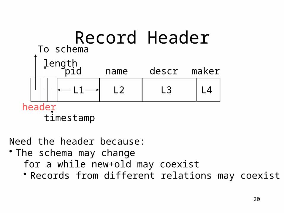
Record Header
L1 L2 L3 L4
To schema
length
timestamp
Need the header because:• The schema may change
for a while new+old may coexist• Records from different relations may coexist
header
pid name descr maker

21
Variable Length Records
L1 L2 L3 L4
Other header information
length
Place the fixed fields first: F1Then the variable length fields: F2, F3, F4Null values take 2 bytes onlySometimes they take 0 bytes (when at the end)
header pid name descr maker

22
BLOB
• Binary large objects• Supported by modern database systems• E.g. images, sounds, etc.• Storage: attempt to cluster blocks together
CLOB = character large object• Supports only restricted operations

23
File Organizations
• Heap (random order) files: Suitable when typical access is a file scan retrieving all records.
• Sorted Files: Best if records must be retrieved in some order, or only a `range’ of records is needed.
• Indexes: Data structures to organize records via trees or hashing. – Like sorted files, they speed up searches for a subset of
records, based on values in certain (“search key”) fields– Updates are much faster than in sorted files.

24
Modifications: Insertion
• File is unsorted: add it to the end (easy )• File is sorted:
– Is there space in the right block ?• Yes: we are lucky, store it there
– Is there space in a neighboring block ?• Look 1-2 blocks to the left/right, shift records
– If anything else fails, create overflow block

25
Modifications: Deletions
• Free space in block, shift records• Maybe be able to eliminate an overflow
block• Can never really eliminate the record,
because others may point to it– Place a tombstone instead (a NULL record)

26
Modifications: Updates
• If new record is shorter than previous, easy
• If it is longer, need to shift records, create overflow blocks

Dan Suciu -- CSEP544 Fall 2010
Index
• A (possibly separate) file, that allows fast access to records in the data file
• The index contains (key, value) pairs:– The key = an attribute value– The value = one of:
• pointer to the recordsecondary index• or the record itself primary index
27Note: “key” (aka “search key”) again means something else

28
Index Classification
• Clustered/unclustered– Clustered = records close in index are close in data– Unclustered = records close in index may be far in data
• Primary/secondary– Meaning 1:
• Primary = is over attributes that include the primary key• Secondary = otherwise
– Meaning 2: means the same as clustered/unclustered
• Organization: B+ tree or Hash table

Clustered/Unclustered
• Clustered– Index determines the location of indexed records– Typically, clustered index is one where values are
data records (but not necessary)
• Unclustered– Index cannot reorder data, does not determine
data location– In these indexes: value = pointer to data record
CSEP 544 - Spring 2009 29
30
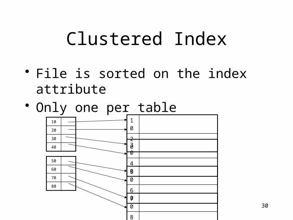
Clustered Index
• File is sorted on the index attribute• Only one per table
10
20
30
40
50
60
70
80
10
20
30
40
50
60
70
80

31
Unclustered Index
• Several per table
10
10
20
20
20
30
30
30
20
30
30
20
10
20
10
30

Dan Suciu -- CSEP544 Fall 2010
32
Clustered vs. Unclustered Index
Data entries(Index File)
(Data file)
Data Records
Data entries
Data Records
CLUSTERED UNCLUSTERED
B+ Tree B+ Tree

CSEP 544 - Spring 2009
Hash-Based Index
18
18
20
22
19
21
21
19
10 21
20 20
30 18
40 19
50 22
60 18
70 21
80 19
H1
h1(sid) = 00
h1(sid) = 11
sid
H2age
h2(age) = 00
h2(age) = 01
Another example of clustered/primary index
Another exampleof unclustered/secondary index
Good for point queries but not range queries
33

34
Alternatives for Data Entry k* in Index
Three alternatives for k*:
• Data record with key value k
• <k, rid of data record with key = k>
• <k, list of rids of data records with key = k>

35
Alternatives 2 and 3
10
10
20
20
20
30
30
30
10
20
30
…

Dan Suciu -- CSEP544 Fall 2010
36
B+ Trees
• Search trees
• Idea in B Trees– Make 1 node = 1 block– Keep tree balanced in height
• Idea in B+ Trees– Make leaves into a linked list: facilitates range
queries

37
• Parameter d = the degree• Each node has >= d and <= 2d keys (except
root)
• Each leaf has >=d and <= 2d keys:
B+ Trees Basics
30 120 240
Keys k < 30Keys 30<=k<120 Keys 120<=k<240 Keys 240<=k
40 50 60
40 50 60
Next leaf

B+ Tree Example
80
20 60 100 120 140
10 15 18 20 30 40 50 60 65 80 85 90
10 15 18 20 30 40 50 60 65 80 85 90
d = 2 Find the key 40

B+ Tree Example
80
20 60 100 120 140
10 15 18 20 30 40 50 60 65 80 85 90
10 15 18 20 30 40 50 60 65 80 85 90
d = 2 Find the key 40
40 80

B+ Tree Example
80
20 60 100 120 140
10 15 18 20 30 40 50 60 65 80 85 90
10 15 18 20 30 40 50 60 65 80 85 90
d = 2 Find the key 40
40 80
20 < 40 60

B+ Tree Example
80
20 60 100 120 140
10 15 18 20 30 40 50 60 65 80 85 90
10 15 18 20 30 40 50 60 65 80 85 90
d = 2 Find the key 40
40 80
20 < 40 60
30 < 40 40

Dan Suciu -- CSEP544 Fall 2010
42
Using a B+ Tree
• Exact key values:– Start at the root– Proceed down, to the leaf
• Range queries:– As above– Then sequential traversal
Select nameFrom PeopleWhere age = 25
Select nameFrom PeopleWhere 20 <= age and age <= 30
Index on People(age)

Dan Suciu -- CSEP544 Fall 2010
Which queries can use this index ?
43
Select *From PeopleWhere name = ‘Smith’ and zipcode = 12345
Index on People(name, zipcode)
Select *From PeopleWhere name = ‘Smith’
Select *From PeopleWhere zipcode = 12345

Dan Suciu -- CSEP544 Fall 2010
44
B+ Tree Design
• How large d ?• Example:
– Key size = 4 bytes– Pointer size = 8 bytes– Block size = 4096 byes
• 2d x 4 + (2d+1) x 8 <= 4096• d = 170

Dan Suciu -- CSEP544 Fall 2010
45
B+ Trees in Practice
• Typical order: 100. Typical fill-factor: 67%– average fanout = 133
• Typical capacities– Height 4: 1334 = 312,900,700 records– Height 3: 1333 = 2,352,637 records
• Can often hold top levels in buffer pool– Level 1 = 1 page = 8 Kbytes– Level 2 = 133 pages = 1 Mbyte– Level 3 = 17,689 pages = 133 Mbytes

46
Insertion in a B+ Tree
Insert (K, P)• Find leaf where K belongs, insert• If no overflow (2d keys or less), halt• If overflow (2d+1 keys), split node, insert in parent:
• If leaf, keep K3 too in right node• When root splits, new root has 1 key only
K1 K2 K3 K4 K5
P0 P1 P2 P3 P4 p5
K1 K2
P0 P1 P2
K4 K5
P3 P4 p5
parent K3
parent

47
Insertion in a B+ Tree
80
20 60
10 15 18 20 30 40 50 60 65 80 85 90
Insert K=19
100 120 140
10 15 18 20 30 40 50 60 65 80 85 90

48
Insertion in a B+ Tree
80
20 60
10 15 18 20 30 40 50 60 65 80 85 9019
After insertion
100 120 140
10 15 18 19 20 30 40 50 60 65 80 85 90
49
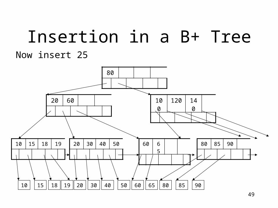
Insertion in a B+ Tree
80
20 60
10 15 18 20 30 40 50 60 65 80 85 9019
Now insert 25
100 120 140
10 15 18 19 20 30 40 50 60 65 80 85 90

50
Insertion in a B+ Tree
80
20 60
20 25 30 40 50
10 15 18 20 25 30 40 60 65 80 85 9019
After insertion
50
100 120 140
10 15 18 19 60 65 80 85 90

51
Insertion in a B+ Tree
80
20 60
10 15 18 20 25 30 40 60 65 80 85 9019
But now have to split !
50
100 120 140
20 25 30 40 5010 15 18 19 60 65 80 85 90

52
Insertion in a B+ Tree
80
20 30 60
10 15 18 19 20 25
10 15 18 20 25 30 40 60 65 80 85 9019
After the split
50
30 40 50
100 120 140
60 65 80 85 90

53
Deletion from a B+ Tree
80
20 30 60
10 15 18 20 25 30 40 60 65 80 85 9019
Delete 30
50
100 120 140
10 15 18 19 20 25 30 40 50 60 65 80 85 90

54
Deletion from a B+ Tree
80
20 30 60
10 15 18 20 25 40 60 65 80 85 9019
After deleting 30
50
40 50
May change to 40, or not
100 120 140
10 15 18 19 20 25 60 65 80 85 90

55
Deletion from a B+ Tree
80
20 30 60
10 15 18 20 25 40 60 65 80 85 9019
Now delete 25
50
100 120 140
40 5010 15 18 19 20 25 60 65 80 85 90

56
Deletion from a B+ Tree
80
20 30 60
20
10 15 18 20 40 60 65 80 85 9019
After deleting 25Need to rebalanceRotate
50
100 120 140
40 5010 15 18 19 60 65 80 85 90

57
Deletion from a B+ Tree
80
19 30 60
10 15 18 20 40 60 65 80 85 9019
Now delete 40
50
100 120 140
19 20 40 5010 15 18 60 65 80 85 90

58
Deletion from a B+ Tree
80
19 30 60
10 15 18 20 60 65 80 85 9019
After deleting 40Rotation not possibleNeed to merge nodes
50
100 120 140
19 20 5010 15 18 60 65 80 85 90
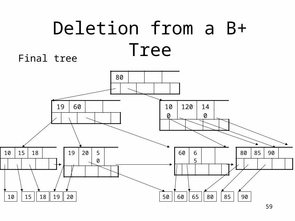
59
Deletion from a B+ Tree
80
19 60
19 20 50
10 15 18 20 60 65 80 85 9019
Final tree
50
100 120 140
10 15 18 60 65 80 85 90

Dan Suciu -- CSEP544 Fall 2010
60
Practical Aspects of B+ Trees
Key compression:• Each node keeps only the from parent
keys• Jonathan, John, Johnsen, Johnson …
– Parent: Jo– Child: nathan, hn, hnsen, hnson, …

Dan Suciu -- CSEP544 Fall 2010
61
Practical Aspects of B+ Trees
Bulk insertion• When a new index is created there are
two options:– Start from empty tree, insert each key one-
by-one– Do bulk insertion – what does that mean ?

62
Practical Aspects of B+ Trees
Concurrency control• The root of the tree is a “hot spot”
– Leads to lock contention during insert/delete
• Solution: do proactive split during insert, or proactive merge during delete– Insert/delete now require only one
traversal, from the root to a leaf– Use the “tree locking” protocol

Dan Suciu -- CSEP544 Fall 2010
63
Summary on B+ Trees
• Default index structure on most DBMS• Very effective at answering ‘point’
queries: productName = ‘gizmo’
• Effective for range queries: 50 < price AND price < 100
• Less effective for multirange: 50 < price < 100 AND 2 < quant < 20

64
Hash Tables
• Secondary storage hash tables are much like main memory ones
• Recall basics:– There are n buckets– A hash function f(k) maps a key k to {0, 1, …, n-
1}– Store in bucket f(k) a pointer to record with key k
• Secondary storage: bucket = block, use overflow blocks when needed

Dan Suciu -- CSEP544 Fall 2010
65
• Assume 1 bucket (block) stores 2 keys + pointers
• h(e)=0• h(b)=h(f)=1• h(g)=2• h(a)=h(c)=3
Hash Table Example
e
b
f
g
a
c
0
1
2
3

Dan Suciu -- CSEP544 Fall 2010
66
• Search for a:• Compute h(a)=3• Read bucket 3• 1 disk access
Searching in a Hash Table
e
b
f
g
a
c
0
1
2
3

Dan Suciu -- CSEP544 Fall 2010
67
• Place in right bucket, if space• E.g. h(d)=2
Insertion in Hash Table
e
b
f
g
d
a
c
0
1
2
3

68
• Create overflow block, if no space• E.g. h(k)=1
• More over-flow blocksmay be needed
Insertion in Hash Table
e
b
f
g
d
a
c
0
1
2
3
k

Dan Suciu -- CSEP544 Fall 2010
69
Hash Table Performance
• Excellent, if no overflow blocks• Degrades considerably when number of
keys exceeds the number of buckets (I.e. many overflow blocks).

Dan Suciu -- CSEP544 Fall 2010
70
Extensible Hash Table
• Allows has table to grow, to avoid performance degradation
• Assume a hash function h that returns numbers in {0, …, 2k – 1}
• Start with n = 2i << 2k , only look at i least significant bits

Dan Suciu -- CSEP544 Fall 2010
71
Extensible Hash Table
• E.g. i=1, n=2i=2, k=4
• Keys:– 4 (=0100)– 7 (=0111)
• Note: we only look at the last bit (0 or 1)
(010)0
(011)1
i=1 1
1
01

Dan Suciu -- CSEP544 Fall 2010
72
Insertion in Extensible Hash Table
• Insert 13 (=1101)(010)0
(011)1
(110)1
i=1 1
1
01

Dan Suciu -- CSEP544 Fall 2010
73
Insertion in Extensible Hash Table
• Now insert 0101
• Need to extend table, split blocks• i becomes 2
(010)0
(011)1
(110)1, (010)1
i=1 1
1
01

Dan Suciu -- CSEP544 Fall 2010
74
Insertion in Extensible Hash Table
(010)0
(11)01
(01)01
i=2 1
2
00011011
(01)11 2
(010)0
(011)1
(110)1, (010)1
i=11
1
01

Dan Suciu -- CSEP544 Fall 2010
75
Insertion in Extensible Hash Table
• Now insert 0000, 1110
• Need to split block
(010)0
(000)0, (111)0
(11)01
(01)01
i=2 1
2
00011011
(01)11 2

76
Insertion in Extensible Hash Table
• After splitting the block
(01)00
(00)00
(11)01
(01)01
i=2 2
200011011
(01)11 2
(11)10 2
1 became 2

Dan Suciu -- CSEP544 Fall 2010
77
Extensible Hash Table
• How many buckets (blocks) do we need to touch after an insertion ?
• How many entries in the hash table do we need to touch after an insertion ?

Dan Suciu -- CSEP544 Fall 2010
78
Performance Extensible Hash Table
• No overflow blocks: access always one read
• BUT:– Extensions can be costly and disruptive– After an extension table may no longer fit
in memory

Dan Suciu -- CSEP544 Fall 2010
79
Linear Hash Table
• Idea: extend only one entry at a time• Problem: n= no longer a power of 2• Let i be such that 2i <= n < 2i+1
• After computing h(k), use last i bits:– If last i bits represent a number > n,
change msb from 1 to 0 (get a number <= n)

Dan Suciu -- CSEP544 Fall 2010
80
Linear Hash Table Example
• n=3(01)00
(11)00
(10)10
i=2
000110
(01)11 BIT FLIP

Dan Suciu -- CSEP544 Fall 2010
81
Linear Hash Table Example
• Insert 1000: overflow blocks…
(01)00
(11)00
(10)10
i=2
000110
(01)11
(10)00

Dan Suciu -- CSEP544 Fall 2010
82
Linear Hash Tables
• Extension: independent on overflow blocks
• Extend n:=n+1 when average number of records per block exceeds (say) 80%

83
Linear Hash Table Extension
• From n=3 to n=4
• Only need to touchone block (which one ?)
(01)00
(11)00
(10)10
i=2
000110
(01)11(01)11
(01)11
i=2
000110
(10)10
(01)00
(11)00
n=11

84
Linear Hash Table Extension
• From n=3 to n=4 finished
• Extension from n=4to n=5 (new bit)
• Need to touch everysingle block (why ?) (01)11
i=2
000110
(10)10
(01)00
(11)00
11

Indexes in Postgres
85
CREATE INDEX V1_N ON V(N)
CREATE TABLE V(M int, N varchar(20), P int);
CREATE INDEX V2 ON V(P, M)
CREATE INDEX VVV ON V(M, N)
CLUSTER V USING V2 Makes V2 clustered
Database Tuning Overview
• The database tuning problem• Index selection (discuss in detail)• Horizontal/vertical partitioning (see
lecture 3)• Denormalization (discuss briefly)
86CSEP 544 - Spring 2009

CSEP 544 - Spring 2009
Levels of Abstraction in a DBMS
Disk
Physical Schema
Conceptual Schema
External Schema External Schema External Schema
a.k.a logical schemadescribes stored datain terms of data model
includes storage detailsfile organizationindexes
viewsaccess control
87

The Database Tuning Problem
• We are given a workload description– List of queries and their frequencies– List of updates and their frequencies– Performance goals for each type of query
• Perform physical database design– Choice of indexes– Tuning the conceptual schema
• Denormalization, vertical and horizontal partition
– Query and transaction tuning
88CSEP 544 - Spring 2009

The Index Selection Problem
• Given a database schema (tables, attributes)• Given a “query workload”:
– Workload = a set of (query, frequency) pairs– The queries may be both SELECT and updates– Frequency = either a count, or a percentage
• Select a set of indexes that optimizes the workload
89
In general this is a very hard problem CSEP 544 - Spring 2009

Index Selection: Which Search Key
• Make some attribute K a search key if the WHERE clause contains:– An exact match on K– A range predicate on K– A join on K
90CSEP 544 - Spring 2009

Dan Suciu -- CSEP544 Fall 2010
Index Selection Problem 1
91
V(M, N, P);
SELECT * FROM VWHERE N=?
SELECT * FROM VWHERE P=?
100000 queries: 100 queries:
Your workload is this
What indexes ?

Dan Suciu -- CSEP544 Fall 2010
Index Selection Problem 1
92
V(M, N, P);
SELECT * FROM VWHERE N=?
SELECT * FROM VWHERE P=?
100000 queries: 100 queries:
Your workload is this
A: V(N) and V(P) (hash tables or B-trees)

Dan Suciu -- CSEP544 Fall 2010
Index Selection Problem 2
93
V(M, N, P);
SELECT * FROM VWHERE N>? and N<?
SELECT * FROM VWHERE P=?
100000 queries: 100 queries:
Your workload is this
INSERT INTO VVALUES (?, ?, ?)
100000 queries:
What indexes ?

Dan Suciu -- CSEP544 Fall 2010
Index Selection Problem 2
94
V(M, N, P);
SELECT * FROM VWHERE P=?
100000 queries: 100 queries:
Your workload is this
INSERT INTO VVALUES (?, ?, ?)
100000 queries:
SELECT * FROM VWHERE N>? and N<?
A: definitely V(N) (must B-tree); unsure about V(P)

Dan Suciu -- CSEP544 Fall 2010
Index Selection Problem 3
95
V(M, N, P);
SELECT * FROM VWHERE N=?
SELECT * FROM VWHERE N=? and P>?
100000 queries: 1000000 queries:
Your workload is this
INSERT INTO VVALUES (?, ?, ?)
100000 queries:
What indexes ?

Index Selection Problem 3
96
V(M, N, P);
SELECT * FROM VWHERE N=?
SELECT * FROM VWHERE N=? and P>?
100000 queries: 1000000 queries:
Your workload is this
INSERT INTO VVALUES (?, ?, ?)
100000 queries:
A: V(N, P)

Dan Suciu -- CSEP544 Fall 2010
Index Selection Problem 4
97
V(M, N, P);
SELECT * FROM VWHERE P>? and P<?
1000 queries: 100000 queries:
Your workload is this
SELECT * FROM VWHERE N>? and N<?
What indexes ?

Dan Suciu -- CSEP544 Fall 2010
Index Selection Problem 4
98
V(M, N, P);
SELECT * FROM VWHERE P>? and P<?
1000 queries: 100000 queries:
Your workload is this
SELECT * FROM VWHERE N>? and N<?
A: V(N) secondary, V(P) primary index

Dan Suciu -- CSEP544 Fall 2010
The Index Selection Problem
• SQL Server– Automatically, thanks to AutoAdmin project– Much acclaimed successful research project from
mid 90’s, similar ideas adopted by the other major vendors
• PostgreSQL– You will do it manually, part of homework 5– But tuning wizards also exist
99

Dan Suciu -- CSEP544 Fall 2010
Index Selection: Multi-attribute Keys
Consider creating a multi-attribute key on K1, K2, … if
• WHERE clause has matches on K1, K2, …– But also consider separate indexes
• SELECT clause contains only K1, K2, ..– A covering index is one that can be used
exclusively to answer a query, e.g. index R(K1,K2) covers the query: 100SELECT K2 FROM R WHERE K1=55

To Cluster or Not
• Range queries benefit mostly from clustering
• Covering indexes do not need to be clustered: they work equally well unclustered
101CSEP 544 - Spring 2009

Dan Suciu -- CSEP544 Fall 2010
102
Percentage tuples retrieved
Cost
0 100
Sequential scan
Clustered index
Unc
lust
ered
inde
x
SELECT *FROM RWHERE K>? and K<?

Hash Table v.s. B+ tree
• Rule 1: always use a B+ tree
• Rule 2: use a Hash table on K when:– There is a very important selection query on
equality (WHERE K=?), and no range queries– You know that the optimizer uses a nested loop
join where K is the join attribute of the inner relation (you will understand that in a few lectures)

Balance Queries v.s. Updates
• Indexes speed up queries– SELECT FROM WHERE
• But they usually slow down updates:– INSERT, DELECTE, UPDATE– However some updates benefit from
indexes
UPDATE R SET A = 7 WHERE K=55

Dan Suciu -- CSEP544 Fall 2010
Tools for Index Selection
• SQL Server 2000 Index Tuning Wizard• DB2 Index Advisor
• How they work:– They walk through a large number of
configurations, compute their costs, and choose the configuration with minimum cost
105

Dan Suciu -- CSEP544 Fall 2010
Tuning the Conceptual Schema
• Denormalization
• Horizontal Partitioning
• Vertical Partitioning
106

Dan Suciu -- CSEP544 Fall 2010
Denormalization
107
SELECT x.pid, x.pnameFROM Product x, Company yWHERE x.cid = y.cid and x.price < ? and y.city = ?
Product(pid, pname, price, cid)Company(cid, cname, city)
A very frequent query:
How can we speed up this query workload ?

Dan Suciu -- CSEP544 Fall 2010
Denormalization
108
Product(pid, pname, price, cid)Company(cid, cname, city)
Denormalize:ProductCompany(pid,pname,price,cname,city)
INSERT INTO ProductCompany SELECT x.pid, x.pname,.price, y.cname, y.city FROM Product x, Company y WHERE x.cid = y.cid

Dan Suciu -- CSEP544 Fall 2010
Denormalization
109
SELECT x.pid, x.pnameFROM Product x, Company yWHERE x.cid = y.cid and x.price < ? and y.city = ?
Next, replace the query
SELECT pid, pnameFROM ProductCompanyWHERE price < ? and city = ?

Issues with Denormalization
110
• It is no longer in BCNF– We have the hidden FD: cid cname, city
• When Product or Company are updated, we need to propagate updates to ProductCompany– Use RULE in postgres (see below)– Or use a trigger on a different RDBMS
• Sometimes cannot modify the query– What do we do then ?

Dan Suciu -- CSEP544 Fall 2010
Denormalization Using Views
111
INSERT INTO ProductCompany SELECT x.pid, x.pname,.price, y.cid, y.cname, y.city FROM Product x, Company y WHERE x.cid = y.cid;
DROP Product; DROP Company;
CREATE VIEW Product AS SELECT pid, pname, price, cid FROM ProductCompany
CREATE VIEW Compnay AS SELECT DISTINCT cid, cname, city FROM ProductCompany

Dan Suciu -- CSEP544 Fall 2010
Denormalization Using Views
112
SELECT x.pid, x.pnameFROM Product x, Company yWHERE x.cid = y.cid and x.price < ? and y.city = ?
Keep the query unchaged
What does the system do ?

Dan Suciu -- CSEP544 Fall 2010
Denormalization Using Views
• In postgres the rewritten query is non-minimal:– Means: has redundant joins– To see this in postgres, type “explain . . .”– For Project 2: it’s OK to use
denormalization using views (don’t forget indexes); performance is reasonable
• SQL Server does a better job with this query
113

Dan Suciu -- CSEP544 Fall 2010
Horizontal Partition
Horizontal partition on price < 10 and price >= 10
• When few products have price < 10 but most queries are about these products
114
Product(pid, pname, price, cid)

Dan Suciu -- CSEP544 Fall 2010
Horizontal Partition
115
INSERT INTO CheapProduct . . . WHERE price<10INSERT INTO ExpensiveProduct . . . WHERE price >=10
DROP Product
CREATE VIEW Product AS (select * from cheapProduct) UNION ALL (select * from expensiveProduct)

Dan Suciu -- CSEP544 Fall 2010
Horizontal Partition
116
SELECT *FROM ProductWHERE price = 2
Which of the tables cheapProduct and
expensiveProduct does it touch ?

Dan Suciu -- CSEP544 Fall 2010
Horizontal Partition
• The query will touch both cheapProduct and expensiveProduct because we haven’t told the system the partition criteria (price < 10 and >= 10)
• We can do this in two ways:– As a predicate in the view definition– As a constraint in the table definition
117

Dan Suciu -- CSEP544 Fall 2010
Partition Criteria As View Predicates
118
CREATE VIEW Product AS (select * from cheapProduct where price < 10) UNION ALL (select * from expensiveProduct where price >= 10)
SQL Server correctly optimizes the query, but postgres doesn’t

Dan Suciu -- CSEP544 Fall 2010
Partition Criteria As Table Constraints
119
CREATE TABLE CheapProduct ( pid int primary key not null, pname varchar(20) not null, price int not null, CHECK (price < 10));
CREATE TABLE ExpesniveProduct ( . . . . CHECK (price >= 10));
If you set “constraint_exclusion = on” in postgresql.conf,then postgres optimizes this fine.

Dan Suciu -- CSEP544 Fall 2010
Updates Through Views
• Product is a view:– What should “INSERT INTO Product” do ?
• Sometime it is possible for the system to figure out which base tables to update
• If not, then use RULES or TRIGGERS120

Dan Suciu -- CSEP544 Fall 2010
RULES in Postgres
121
CREATE [ OR REPLACE ] RULE name AS ON event TO table [ WHERE condition ] DO [ ALSO | INSTEAD ] { NOTHING | command | ( command ; command ... ) }
Where name = a name for the rule event = SELECT, INSERT, UPDATE, or DELETE command = SELECT, INSERT, UPDATE, DELETE use new for the new tuple, and old for the old tuple

Dan Suciu -- CSEP544 Fall 2010
RULES in Postgres
122
CREATE OR REPLACE RULE productInsertRule AS ON INSERT TO Product DO INSTEAD (INSERT INTO cheapProducts SELECT DISTINCT new.pid, new.pname, new.price FROM anyDummyTablePreferablyWithOneTuple WHERE new.price < 10; INSERT INTO expensiveProducts SELECT DISTINCT new.pid, new.pname, new.price FROM anyDummyTablePreferablyWithOneTuple WHERE new.price >= 10);

Dan Suciu -- CSEP544 Fall 2010
RULES in Postgres
123
CREATE OR REPLACE RULE productDeleteRule AS ON DELETE TO Product DO INSTEAD (DELETE FROM cheapProducts WHERE pid = old.pid DELETE FROM expensiveProducts WHERE pid = old.pid);

Dan Suciu -- CSEP544 Fall 2010
Vertical Partition
124
Split vertically into:
Product1(pid, name, price)
Product2(pid, description)
Define Product as view
Product(pid, pname, price, description)
Varchar(500)

Dan Suciu -- CSEP544 Fall 2010
Vertical Partition
125
CREATE VIEW Product AS (select x.pid, x.pname, x.price, y.description from Product1 x, Product 2 y where x.pid = y.pid)

Dan Suciu -- CSEP544 Fall 2010
Vertical Partition
126
SELECT pid, pnameFROM ProductWHERE price > 20
Now consider a query on Product:
Which tables are touched by the system ?

Dan Suciu -- CSEP544 Fall 2010
Vertical Partition
• SQL Server does the right thing:– Touches only product1
• But postgres insists on joining product1 with product2 instead– I couldn’t figure out how to coerce postgres
to optimize this query– 10 bonus points for whoever finds out first !– In the meantime, we will cheat like this:
127

Dan Suciu -- CSEP544 Fall 2010
128
CREATE VIEW Product AS select pid, pname, price, ‘blah’ as description from Product1

Dan Suciu -- CSEP544 Fall 2010
129
NOT DISCUSSED IN CLASS

Security in SQL
• Discretionary access control in SQL
• Using views for security
CSEP 544 - Spring 2009 130

131
Discretionary Access Control in SQL
GRANT privileges ON object TO users [WITH GRANT OPTIONS]
privileges = SELECT | INSERT(column-name) | UPDATE(column-name) | DELETE | REFERENCES(column-name)object = table | attribute

132
Examples
GRANT INSERT, DELETE ON Customers TO Yuppy WITH GRANT OPTIONS
Queries allowed to Yuppy:
Queries denied to Yuppy:
INSERT INTO Customers(cid, name, address) VALUES(32940, ‘Joe Blow’, ‘Seattle’)
DELETE Customers WHERE LastPurchaseDate < 1995
SELECT Customer.addressFROM CustomerWHERE name = ‘Joe Blow’

133
Examples
GRANT SELECT ON Customers TO Michael
Now Michael can SELECT, but not INSERT or DELETE

134
Examples
GRANT SELECT ON Customers TO Michael WITH GRANT OPTIONS
Michael can say this: GRANT SELECT ON Customers TO Yuppi
Now Yuppi can SELECT on Customers

135
Examples
GRANT UPDATE (price) ON Product TO Leah
Leah can update, but only Product.price, but not Product.name

136
Examples
GRANT REFERENCES (cid) ON Customer TO Bill
Customer(cid, name, address, balance)Orders(oid, cid, amount) cid= foreign key
Now Bill can INSERT tuples into Orders
Bill has INSERT/UPDATE rights to Orders.BUT HE CAN’T INSERT ! (why ?)

137
Views and Security
CREATE VIEW PublicCustomers SELECT Name, Address FROM CustomersGRANT SELECT ON PublicCustomers TO Fred
David says
Name Address Balance
Mary Huston 450.99
Sue Seattle -240
Joan Seattle 333.25
Ann Portland -520
David owns
Customers:Fred is notallowed tosee this

138
Views and Security
Name Address Balance
Mary Huston 450.99
Sue Seattle -240
Joan Seattle 333.25
Ann Portland -520
CREATE VIEW BadCreditCustomers SELECT * FROM Customers WHERE Balance < 0GRANT SELECT ON BadCreditCustomers TO John
David says
David owns
Customers: John isallowed to
see only <0balances

139
Views and Security• Each customer should see only her/his record
CREATE VIEW CustomerMary SELECT * FROM Customers WHERE name = ‘Mary’GRANT SELECT ON CustomerMary TO Mary
Doesn’t scale.
Need row-level access control !
Name Address Balance
Mary Huston 450.99
Sue Seattle -240
Joan Seattle 333.25
Ann Portland -520
David says
CREATE VIEW CustomerSue SELECT * FROM Customers WHERE name = ‘Sue’GRANT SELECT ON CustomerSue TO Sue
. . .

140
Revocation
REVOKE [GRANT OPTION FOR] privileges ON object FROM users { RESTRICT | CASCADE }
Administrator says:
REVOKE SELECT ON Customers FROM David CASCADE
John loses SELECT privileges on BadCreditCustomers

141
Revocation
Joe: GRANT [….] TO Art …Art: GRANT [….] TO Bob …Bob: GRANT [….] TO Art …Joe: GRANT [….] TO Cal …Cal: GRANT [….] TO Bob …Joe: REVOKE [….] FROM Art CASCADE
Same privilege,same object,
GRANT OPTION
What happens ??

142
Revocation
Admin
Joe Art
Cal Bob
0
1
234
5
Revoke
According to SQL everyone keeps the privilege

Summary of SQL Security
Limitations:• No row level access control• Table creator owns the data: that’s unfair !• Today the database is not at the center of
the policy administration universe
143