1

Lecture 6.

•Maximum Likelihood

•Conditional Probability and two-stage experiments

•Markov Chains (introduction).

• Markov Chains with Mathematica

•Bayes formula.

•Student’s presentation

2

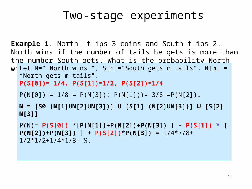
Two-stage experiments

Example 1. North flips 3 coins and South flips 2. North wins if the number of tails he gets is more than the number South gets. What is the probability North will win?

Let N=" North wins ", S[n]=“South gets n tails", N[m] = “North gets m tails".P(S[0])= 1/4. P(S[1])=1/2, P(S[2])=1/4

P(N[0]) = 1/8 = P(N[3]); P(N[1]))= 3/8 =P(N[2]).

N = [S0 (N[1]UN[2]UN[3])] U [S[1] (N[2]UN[3])] U [S[2] N[3]]

P(N)= P(S[0]) *[P(N[1])+P(N[2])+P(N[3]) ] + P(S[1]) * [ P(N[2])+P(N[3]) ] + P(S[2])*P(N[3]) = 1/4*7/8+ 1/2*1/2+1/4*1/8= ½.

3

Another form of the same equation:

P(N) = P(N*S[0]) + P(N*S[1]) + P(N*S[2]) =

Sum[ P(N*S[ n ] ), { n, 0, 2} ]

= Sum[ P(N | S[ n ] )* P(S[ n ] ), { n, 0, 2}

Probability that South gets n heads and North wins

Conditional Probability of N winning given that S has I heads

4

This formula is sometimes called the law of the total probability

We think of such an experiment as occurring in two stages. The first stage determines which of B's occur, and when Bi occurs on the first stage, A occurs with probability P(A|Bi) on the second.

Suppose that B1,B2,...Bk is a collection of k disjoined events whose union is . Using the fact that the sets A∩Bn are disjoined , and the multiplication rule

for the conditional probability , P(AB) = P(A|B) P(B), we have

)1.6()()|()()(11

nn

k

nn

k

nBPBAPBAPAP

5

Example 2. Roll a die and then flip that number of coins. What is the probability of 3H= “We get exactly 3 Heads”?

Let Bi = “The die shows i”. P(Bi) = 1/6 for i=1,2,..6.

Now find the conditional probabilities. P(3H|B1)=P(3H|B2)= 0. P(3H|B3) = 1/23; P(3H|B4)= C4,3 /24; P(3H|B5)= C5,3 /25; P(3H|B6) = C6,3 /26.

So plugging into Eq. (1) we find:

P(3H) = 1/6 [ 1/8 + 4/16 + 10/32 + 20/64] = 1/6

6

An example from Genetics

Each hereditary characteristic is carried by a pair of genes, so that each offspring gets one chromosome from its mother and one from its father. We will consider a case in which each gene can take only two forms called alleles, which we denote by a and A. An example from a pioneering work of Gregor Mendel is A="smooth skin" and a ="wrinkled skin" for the pea plants. In this case A is dominant over a, which means that Aa individuals will have a smooth skin.

Let us start from an idealized infinite population with following distribution of genotypes

AA Aa aa

0 0 0

where the proportions 0, 0 and 0 sum to 1.

7

If we assume that random mating occurs then eachnew individual picks two parents at random from population and picks allele at random from two carried by each parent.

Then, the first allele will be A with probability

p1=0+0/2 and a with probability 1-p1= 0+ 0/2 .

The second allele will be independent and have the same distribution, so that the first generation of offspring will be

AA Aa aa

1=p12 1=2p1(1-p1) 1= (1-p1)2

Note that this distribution is determined by the relative weight p1 of A (or a)

in the population ( which can be expressed through 0 and 0 ) while the original distribution (or the choice of 0 and 0) is arbitrary.

Let us now use this distribution to calculate the second generation of offspring. A will now have a probability p2 = p1

2 + p1(1-p1) = p1 (!)

AA Aa aa

0 0 0

8

, So the proportions of the second generation of offspring will be

2=p22=p1

2= 12=2p2(1-p2)= 1 2= (1-p2)2= 1

-exactly the same as in the first generation

This result is called the Hardy-Weinberg Theorem.

We can see that the distribution of genotypes reaches its equilibrium in one generation of offspring starting from an arbitrary distribution. It means that if the proportion of dominant alleles A is p then the proportion of genotypes (uniquely determined by p) will be

AA Aa aa

p2 2p(1-p) (1-p)2

9

To illustrate its use suppose that in a population of pea plant 10% have wrinkled skin (aa) and 90% have smooth skin (AA or Aa). Using the table above, we can find the proportions of three genotypes.

The fraction p of alleles we find from the condition + =0.9 leading to 2p-p2=0.9, p=0.684. As a result, the proportions are:

=p2=0.46 (AA), =2p(1-p)= 0.44 (Aa), =(1-p)2=0.1(aa).

10

Problems (working in groups):

1. You are going to meet a friend in the airport. You know that the plane is late 70% of the time when it rains, and 20 % when it does not rain. The weather forecast calls for a 40% chance of rain. What is the probability that the plain will be late?

A=“plain will be late”; R=“it will rain”; S= “it won’t rain”

2. How can 5 black and 5 white balls be put into two urns to maximize the probability that a white ball is drawn when we draw from a randomly-chosen urn (try solving it with Mathematica).

Solution: Using the law of total probability, we find:P(A)= P(A|R)*P(R) + P(A|S)P(S) = 0.7*0.4+ 0.2* 0.6= 0.28+0.12= 0.4.

11

See the solution in Mathematica/Class_2Boxes_solution.nb

12

Two-state Markov Chains

In 1907, Russian mathematician A.A. Markov began study chance processes in which the outcome of a given experiment can affect the outcome of the next experiment. We consider here a simple example of such process leaving a more detailed discussion for future

Suppose that there are two brands of bread, A and B, and that on each purchase a customer changes brands with probability p(change)=2/7 ≡ p and buys the same brand with probability p(stay)=5/7 ≡ 1-p. Let fk be the fraction that buys brand A on their k-th purchase and suppose f1=1/3.

Compute f1,f2, …

Let Ak=" a customer bought brand A on the k-th step".

We do not know explicitly the probability P(Ak), but we know that it depends on the previous step:

13

P(Ak)= P(Ak-1)(1-p)+P(Bk-1 )p = 5/7 P(Ak-1) + 2/7[1- P(Ak-1)].

Using the frequency definition of probability, we can present it as:

1 1 1 1

5 21 1 1 1

7 7( ) ( ) ( ) ( _ )k k k k kf p f p f f f Mark

This is a typical example of a "recursive equation". It can be solved step by step, but we prefer to use Mathematica

This is how the recursive equation is solved:Mathematica 4 .lnk

f[k_] := (5/7) f[k-1] + (1/7)(1 – f[k-1]);f[1] = 1/3.;

{0.333333,0.428571,0.469388,0.48688,0.494377,0.49759,0.498967,0.499557,0.49981,0.499919,0.499965,0.499985,0.499994,0.499997,0.499999}

a = Table[f[k], {k, 1, 15}]

stay change

14

0 2 4 6 8 10 12 14

0.35

0.375

0.4

0.425

0.45

0.475

0.5

The population rapidly approaches 0.5.

Group work:Why is it 0.5? Does it depend on the initial value f1 ? On the probability p? Solve the same equation with f1 =0.1, then change p to p = ¼. Does it change the results? –Practice with Markov0 and Markov1

15

As you noticed, the equilibrium population is always 0.5, regardless the values of p and f[1].

Let us now generalize the model. Consider a system that has two states: A and B, and changes its states with probabilities:

Prob(AB )= p, Prob(A A)=1-p, Prob(B A )= q, Prob(B B)=1-q.Let fk be a share of the total population belonging to the state A on the k-th step of evolution. The recursive equation for this model becomes

f[p_,q_,k_]:=(1-p)f[p,q,k-1]+q(1-f[p,q,k-1]); Mark_2

f[p_,q_,1]=1/3; Mark_3

(see Markov2.nb)

Solve this equation for ten steps, k = (1,10) , and with various combinations of probabilities: {p,q}= {0.2,0.4},{0.2,0.5},{0.3,0.6}, {0.3,0.3}. Try to figure out how the asymptotic value of fk depends on p , q and f1

16

You will find (Markob2.nb) that fkq/(p+q). This result can be derived analytically.

Assuming in Eq. Mark_2 fk-1=fk= r, we find:

r = (1-p)r +(1-r)q which leads to

r= q/(p+q).

Final comments.

The 2-state Markov chain is a simplest example of the Markov Chains.

In general, if there are m states, the transition between the states is described by a “transition matrix” pij.. For a uniform Markov process, pij does not depend on the step number (on the “discrete time coordinate”), although in the reality its not always the case.

17

Bayes Formula

Conditioning usually implies that the probability of the following step can be found given that the previous step has occurred. Very often, however, the question is reversed: given the result, find the probability that its certain precondition occurred.

18

Suppose that B can only occur in combination with one of m events A1,A2,....,Am any two of which are mutually exclusive. Suppose that P(Ai) and P(B| Ai) are known. We then have B=BA1+BA2+...+B Am and

mP(B)= P(A ) ( | )

kk=1P B A

k

2( ) ( | )

P(A |B)= ( )/ ( ) ( )n ( ) ( | )P A P B An nP A B P Bn P A P B Ai i

Then,

This is the Bayes Formula.

It allows us to estimate probabilities of occurring of any of the events Ak each of whom can lead to the event B, given that B occurred.

19

Graphical interpretation of Bayes formula.

There are m different roots leading to B. The probability of reaching B through the n-th root equals P(An)P(B|An), the probability of choosing this root by the probability that it was traveled successfully. We assume that all P(An) and P(B|An) are known. Assuming that B was reached, the Byes formula allows to calculate a probability that it was done through a certain root:

P(getting to B by the n-th root)P(n-th root was chosen | B was reached)=P(getting to B by any one of m roots)

BA1

A2

An Am

P(An|B)P(B|An)

20

Example 1.

1

2

3

Box 1 contains 2 red and 3 blue balls; Box 2, 4 red and one blue; and Box 3, 3 red and 4 blue.

A box is selected at random, and a ball drawn at random is found to be red. Find the probability that box 1 was selected.

Each box can be chosen with P(Box n)= 1/3. We are looking for the probability P(Box1|A) that Box1 was selected given A = “the ball was red”.

We will be using Eq. 2 translated into our events

First, find P(A) = 1/3*2/5 + 1/3*4/5+1/3*3/7=0.54 Second, find P(Box1*A)= 1/3*2/5 =0.13

Finally, P(Box1|A) =0.13/0.54~ 0.25

1 11 ( ) ( | )P(Box1|A)= ( )/ ( )( ) ( | )

P Box P A BoxP Box A P AP Boxj P A Boxj

21

Example 2: Exit Polls.

In the California gubernatorial elections in 1982, several TV stations predicted, on the basis of exit polls analysis, that Tom Bradley, would win the election. When the votes were counted, however, he lost by a considerable margin.

What happened?

•Suppose we chose a person at random. Let B = “The person votes for Bradley”, and suppose P(B) = 0.45 (this is the real probability which is hidden from the analyst). Then, the probability that he voted for his opponent, P(Bc) = 0.55.

•Suppose now that some voters are reluctant to answer the questions. Let A = “The voter stops and answers a question about how she voted”, and suppose that P(A|B)=0.4 and P(A|Bc)=0.3. That is, 40% of Bradley’s voters will respond compared to 30% of his opponent’s voters.

•We are interested in computing P(B|A)- a fraction of voters in our sample that voted for Bradley (this is the measured <apparent> probability available to the analyst).

22

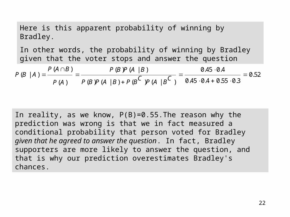
Here is this apparent probability of winning by Bradley.

In other words, the probability of winning by Bradley given that the voter stops and answer the question

0 45 0 40 52

0 45 0 4 0 55 0 3

( ) ( ) ( | ) . .( | ) .

. . . .( ) ( | ) ( ) ( | )( )

P A B P B P A BP B A

C CP B P A B P B P A BP A

In reality, as we know, P(B)=0.55.The reason why the prediction was wrong is that we in fact measured a conditional probability that person voted for Bradley given that he agreed to answer the question. In fact, Bradley supporters are more likely to answer the question, and that is why our prediction overestimates Bradley's chances.

23

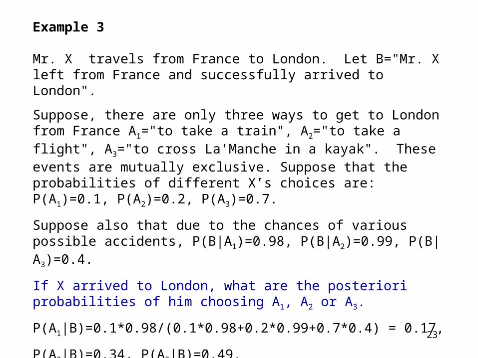
Example 3

Mr. X travels from France to London. Let B="Mr. X left from France and successfully arrived to London".

Suppose, there are only three ways to get to London from France A1="to take a train", A2="to take a flight", A3="to cross La'Manche in a kayak". These events are mutually exclusive. Suppose that the probabilities of different X’s choices are: P(A1)=0.1, P(A2)=0.2, P(A3)=0.7.

Suppose also that due to the chances of various possible accidents, P(B|A1)=0.98, P(B|A2)=0.99, P(B|A3)=0.4.

If X arrived to London, what are the posteriori probabilities of him choosing A1, A2 or A3.

P(A1|B)=0.1*0.98/(0.1*0.98+0.2*0.99+0.7*0.4) = 0.17,

P(A2|B)=0.34, P(A3|B)=0.49.

And what if X did not arrive to London? In such a case P(A1|BC)=0.047 = P(A2|BC), P(A3|BC)=0.991 (check if these values are correct).

24

Example 4 (genetics)

A woman has a brother with hemophilia, but her two parents do not have a decease. It’s known that hemophilia is caused by a recessive gene h on the X chromosome, which implies that mother is the carrier. In such case, the mother has h on one of here X chromosomes and the healthy gene H on the other X chromosome.

Since the woman received one X from her mother and one from her father, there is 50% chance that she is a carrier and 50% chance that her sons will have a decease.

If she has 2 sons without a decease, what’s the probability she is the carrier?

25

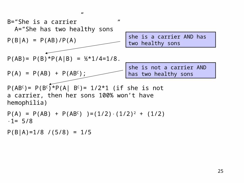
B=“She is a carrier” A=“She has two healthy sons”

P(B|A) = P(AB)/P(A)

P(AB)= P(B)*P(A|B) = ½*1/4=1/8.

P(A) = P(AB) + P(ABC); P(ABC)= P(BC)*P(A| BC)= 1/2*1 (if she is not a carrier, then her sons 100% won’t have hemophilia)

P(A) = P(AB) + P(ABC) )=(1/2)(1/2)2 + (1/2) 1= 5/8

P(B|A)=1/8 /(5/8) = 1/5

she is a carrier AND has two healthy sons

she is not a carrier AND has two healthy sons

26

Home assignment If you have any questions about the HW, please contact me.

1. Read the lecture and work on the problems at pp. 9, 20-25. Make sure you understand the solutions.

2. Solve “Self-Test 6” problems, compare with the solutions.

3. Solve the problems posted on Webct (week 6)

4. Practice with Mathematica. Make sure that everyone goes through the Steps 1-6 and the Markov0-2 files. Based on your HWs submitted lately I can tell that most of you became quite proficient with Mathematica, although some of you practically did not take time to learn this amazing tool and still are walking in darkness.

5. Read and practice with the Maximum Likelihood file (see the link on the page).

27

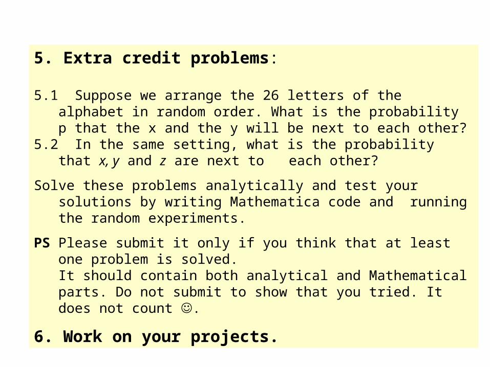
5. Extra credit problems:

5.1 Suppose we arrange the 26 letters of the alphabet in random order. What is the probability p that the x and the y will be next to each other?

5.2 In the same setting, what is the probability that x, y and z are next to each other?

Solve these problems analytically and test your solutions by writing Mathematica code and running the random experiments.

PS Please submit it only if you think that at least one problem is solved.It should contain both analytical and Mathematical parts. Do not submit to show that you tried. It does not count .

6. Work on your projects.