1

Least-Squares Regression

Lecture NotesDr. Rakhmad Arief SiregarUniversiti Malaysia Perlis

Applied Numerical Method for Engineers

Chapter 17

2

3

Curve Fitting

4

Curve Fitting

5

Curve Fitting

6

Simple Statistics

7

Regression

Experimental data

Polynomial fit

Least-squares fit

8

a0 and a1 are coefficients representing the intercept and the slope

e is the error or residual between the model and the observations

Linear Regression

The simplest example of a least-squares approximation is fitting a straight line

exaay 10

9

e is the error or residual, the discrepancy between the true value of y

a0+a1x is the approximate value

Linear Regression

By rearranging:

exaay 10 xaaye 10

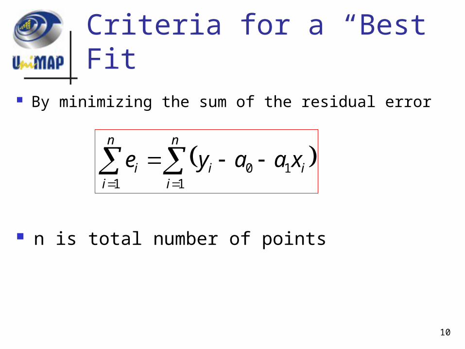
10

n is total number of points

Criteria for a “Best” Fit

By minimizing the sum of the residual error

n

iii

n

ii xaaye

110

1

11

n is total number of points

Criteria for a “Best” Fit

By minimizing the sum of absolute residual error

n

iii

n

ii xaaye

110

1

12

Criteria for a “Best” Fit

By minimizing the sum of the squares of the residuals between the measured y and the y calculated with the linear mode

n

ielimeasuredi

n

ir yyeS

i1

2mod,,

1

2

n

iii

n

ir xaayeS

i1

210

1

2

13

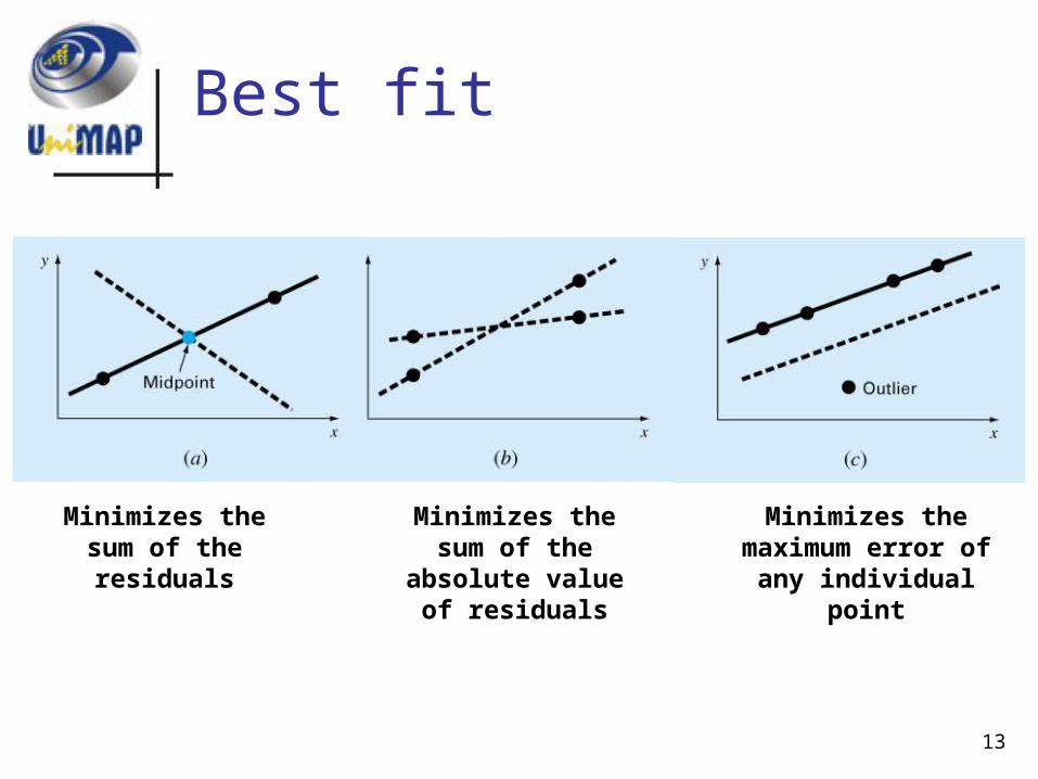
Best fit

Minimizes the sum of the residuals

Minimizes the sum of the

absolute value of residuals

Minimizes the maximum error of

any individual point

14

Least-Squares Fit of a Straight Line

Differentials:

n

iii

n

ir xaayeS

i1

210

1

2

)(2 100

iir xaaya

S

])[(2 101

iiir xxaaya

S

15

Least-Squares Fit of a Straight Line

After several mathematical steps, a0 and a1 will yields:

221

ii

iiii

xxn

yxyxna

xaya 10

Where y and x are the means of y and x, respectively

16

Ex. 17.1

Fit a straight line to the x and y values in the first two columns of Table below.

0

1

2

3

4

5

6

7

0 1 2 3 4 5 6 7 8

17

Ex. 17.1

The following quantities can be computed

5.119ii yx 1402ix

28ix

24iy

7n

47

28x

428571.37

24y

18

Ex. 17.1

a1 and a0 can be computed:

8392857.0)28()140(7

)24(28)5.119(721

a

07142857.0

)4(8392857.0428571.3

0

0

a

a

221

ii

iiii

xxn

yxyxna

xaya 10

19

Ex. 17.1

The least-squares fit is:

xaay 10 xy 8392857.007142857.0

0

1

2

3

4

5

6

7

0 1 2 3 4 5 6 7 8

yi

yi-least

20

Problem 17.4

Use least-squares regression to fit a straight line to:

0

2

4

6

8

10

12

14

0 5 10 15 20

21

Problem 17.4

y = 0.3525x + 4.8515

0

2

4

6

8

10

12

14

0 5 10 15 20

22

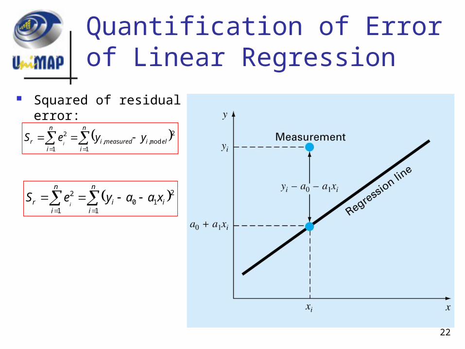
Quantification of Error of Linear Regression

Squared of residual error:

n

iii

n

ir xaayeS

i1

210

1

2

n

ielimeasuredi

n

ir yyeS

i1

2mod,,

1

2

23

Quantification of Error of Linear Regression

If those criteria are met, a “standard deviation” for regression line can be determined as:

where: Sy/x is called standard error of estimate. Subscript y/x means the error is for a predicted

value of y corresponding to a particular value of x

2/ n

Ss r

xy

24

Quantification of Error of Linear Regression

The spread of the data around the mean

The spread of the data around best fit line

n

iii

n

ir xaayeS

i1

210

1

2

n

iit yyS

1

2

25

Quantification of Error of Linear Regression

Small residual errors Large residual errors

26

Quantification of Error of Linear Regression

The difference between the two quantities, St –Sr, quantifies the improvement or error reduction due to describing the data in terms of a straight line.

The difference is normalized to St to yield:

r2 : coefficient of determination r : correlation coefficient

t

rt

S

SSr

2

2222 )()(

))((

iiii

iiii

yynxxn

yxyxnr

27

Ex. 17.2

Compute the total standard deviation, the standard error of the estimate and the correlation coefficient for the data in Ex. 17.1

28

Ex. 17.2

Solution Standard deviation:

Standard error of estimate:

The extent of the improvement is qualified because sy/x < sy the linear regression model has merit

1n

Ss ty

2/ n

Ss r

xy

9457.117

7143.22

ys

7735.027

9911.2/

xys

29

Ex. 17.2

Solution The correlation coefficient:

These results indicate 86.8 percent of the original uncertainty has been explained by the linear model

t

rt

S

SSr

2

868.07143.22

9911.27143.222

r

932.0868.0 r

30

Linearization of Nonlinear Relationships

Linear regression provides a powerful technique for fitting a best line to data.

How about data shown below?

31

Linearization of Nonlinear Relationships

Transformations can be used to express the data in form that is compatible with linear regression

A straight line with a slope 1 and intercept of ln 1

exy lnlnln 11

xey 11

1ln e

xy 11lnln

Exponential equation

By natural logarithm

32

Linearization of Nonlinear Relationships

Power equation

A straight line with a slope 2 and intercept of log 2

22 logloglog xy

22

xy By base-10 logarithm

33

Linearization of Nonlinear Relationships

The saturation-growth-rate equation

A straight line with a slope 3 / 3 and intercept of 1/3

33

3 111

xy

x

xy

33

By inverting

34

35

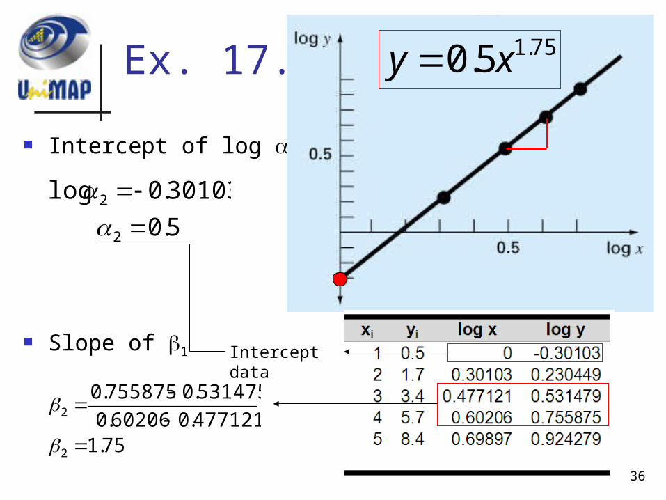
Ex. 17.4

Fit Eq. below to the data in table 17.3 using a logarithmic transformation of the data.

22

xy

36

Ex. 17.4

Intercept of log 2

Slope of 1 Intercept data

30103.0log 2 5.02

75.15.0 xy

75.1477121.060206.0

531475.0755875.0

2

2

37

Polynomial Regression

38

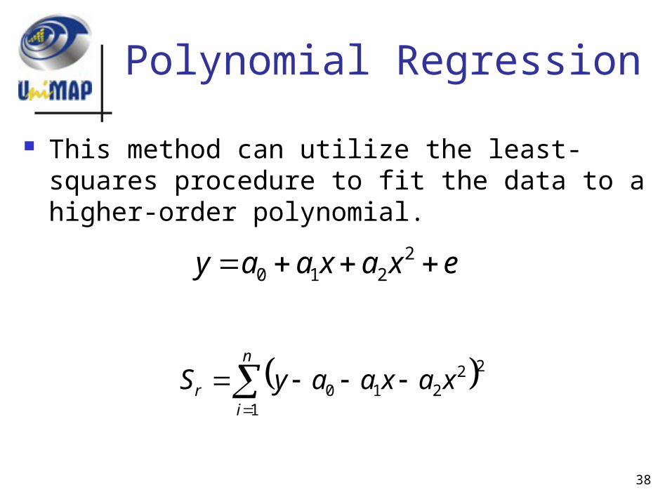
Polynomial Regression

This method can utilize the least-squares procedure to fit the data to a higher-order polynomial.

exaxaay 2210

n

ir xaxaayS

1

22210

39

Polynomial Regression

Derivation with respect to each unknown coefficients of polynomial as in

n

iir xaxaayS

1

22210

2

2100

2 iiir xaxaaya

S

2

2101

2 iiiir xaxaayxa

S

2

2102

2

2 iiiir xaxaayxa

S

40

Polynomial Regression

Derivations can be set equal to zero and rearranged as:

How to solve it?

iiiii yxaxaxax 23

12

0

iiiii yxaxaxax 22

41

30

2

iii yaxaxan 22

10)(

41

Polynomial Regression

In matrix form

What method can be used?

ii

ii

i

iii

iii

ii

yx

yx

y

a

a

a

xxx

xxx

xxn

22

1

0

432

32

2

42

Polynomial Regression

The two dimensional case can be easily extended to an m-th order polynomial as:

The standard error for this case is formulated as

exaxaxaay mm ...2

210

)1(/

mn

Ss r

xy

43

Ex. 17.5

Fit a second-order polynomial to the data in table below:

0

10

20

30

40

50

60

70

0 1 2 3 4 5 6

x

y

44

Ex. 17.5

Solution: m=2, n=6

45

Ex. 17.5

Solution: The simultaneous linear equation are:

ii

ii

i

iii

iii

ii

yx

yx

y

a

a

a

xxx

xxx

xxn

22

1

0

432

32

2

8.2488

6.585

6.152

97922555

2255515

55156

2

1

0

a

a

a

46

Ex. 17.5

Solution: By using gauss elimination it will yield:

a0=2.47857, a1=2.35929 and a2=1.86071

The least-square quadratic equation:

8.2488

6.585

6.152

97922555

2255515

55156

2

1

0

a

a

a

286071.135979.247857.2 xxy

47

12.1)12(6

74657.3/

xys

Ex. 17.5

The standard error:

)1(/

mn

Ss r

xy

48

Ex. 17.5

The coefficient of determination:

t

rt

S

SSr

2

99851.04.2513

74657.34.25132

r

49

Ex. 17.5

0

10

20

30

40

50

60

70

0 1 2 3 4 5 6

x

y

286071.135979.247857.2 xxy

99.851% of the original uncertainty has been explain by the model

50

Assignment 3

Do Problems 17.5, 17.6, 17.7, 17.10 and 17.12

Submit next week

51

Multiple Linear Regression

For this section, two-dimensional case, regression line become a plane

exaxaay 22110

52

Multiple Linear Regression

This method can utilize the least-squares procedure to fit the data to a higher-order polynomial.

exaxaay 2210

n

iiir xaxaayS

1

222110

53

Multiple Linear Regression

Derivation with respect to each unknown coefficients of polynomial as in

iiir xaxaaya

S22110

0

2

iiiir xaxaayxa

S221101

1

2

iiiir xaxaayxa

S221102

2

2

n

iiir xaxaayS

1

222110

54

Multiple Linear Regression

Derivations can be set equal to zero and rearranged as in matrix form

ii

ii

i

iiii

iiii

ii

yx

yx

y

a

a

a

xxxx

xxxx

xxn

2

1

2

1

0

22212

21211

21

55

Multiple Linear Regression

The two dimensional case can be easily extended to an m-th order polynomial as:

The standard error for this case is formulated as

exaxaxaay mm ...2

210

)1(/

mn

Ss r

xy

56

Ex. 17.6

The following data was calculated from equation: y=5+4x1-3x2

Use multiple linear regression to fit this data

57

Ex. 17.6

58

Ex. 17.6

Solution

ii

ii

i

iiii

iiii

ii

yx

yx

y

a

a

a

xxxx

xxxx

xxn

2

1

2

1

0

22212

21211

21

100

5.243

54

544814

485.765.16

145.166

2

1

0

a

a

a

59

Ex. 17.6

solution a0=5, a1=4 and a2=-3

60

Problems 17.17

Use multiple linear regression to fit.

Compute the coefficients, the standard error of estimate and the correlation coefficient

61

Problems 17.17

62

Problems 17.17

Solution

ii

ii

i

iiii

iiii

ii

yx

yx

y

a

a

a

xxxx

xxxx

xxn

2

1

2

1

0

22212

21211

21

x

x

x

a

a

a

xxx

xxx

xxx

2

1

0

63

Nonlinear Regression

The Gauss-Newton method is one algorithm for minimizing the sum of the squares of the residuals between data and nonlinear equation.

imii eaaaxfy ),...,,:( 10

iii exfy )(

For convenience

64

Nonlinear Regression

The nonlinear model can be expanded in a Tailor series around the parameter values and curtailed after the first derivative

Ex. For a two-parameter case:

11

00

1

)()()()( a

a

xfa

a

xfxfxf jiji

jiji

iii exfy )(

65

Nonlinear Regression

It needs to be linearized by substituting

into

It will yields

11

00

1

)()()()( a

a

xfa

a

xfxfxf jiji

jiji

iii exfy )(

eaa

xfa

a

xfxfy jiji

jii

11

00

)()()(

66

Nonlinear Regression

In matrix form

eaa

xfa

a

xfxfy jiji

jii

11

00

)()()(

EAZD j ][

10

1202

1101

//

..

..

..

//

//

afaf

afaf

afaf

Z

nn

j

)(

.

.

.

)(

)(

22

11

nn xfy

xfy

xfy

D

ma

a

a

A

.

.

.1

0

67

Nonlinear Regression

By applying least-square theory to

It will yield in normal equation:

By using ave Eq. we can compute values for:

EAZD j ][

DZAZZ Tjj

Tj ][][][

0,01,0 aaa jj 1,11,1 aaa jj

68

Ex. 17.9