1. radiation · latitude climatology (fig 3.2) has been constructed from hering and borden (l965)...

RADIATION1.

The parameterization of radiative processes has been prepared for NMC by Stephen B. Fels and M. DanielSchwarzkopf of GFDL and their generous contribution of time and effort is gratefully acknowledged. Thissection documents the radiation scheme as implemented at NMC in August 1987. Modeling of bothshortwave and longwave processes include the effects of the major radiatively active atmosphericconstituents - water vapor (H2O), carbon dioxide (CO2), ozone (O3), and clouds. Outputs from theparameterization are forecast model layer radiative heating rates (_K/sec), as well as downward longwave andnet shortwave fluxes (cal cm-2 min-1) at the earth's surface.

The radiation calculations are computationally quite expensive. Using compiler optimized CYBER 205coding, the average radiation computation time for one 18 layer column of atmospheric data is .0031 seconds.This requires approximately 40 seconds of computation time for a rhomboidal-40 grid array. The fastershortwave calculations account for only 18% of this time. Because of their computational expense, radiationcalculations are made only once every 12 hours. Longwave heating rates are held fixed for the entire 12hours; however, provision is made within the forecast model for an approximate diurnal cycle, so shortwaveheating rates and surface radiative fluxes are allowed to change during this interval.

The first part of this report describes the necessary alteration of model temperature and moisture data for theradiation parameterization. Then, climatological surface albedo, ozone concentration, and cloudiness arediscussed. Finally, basic techniques which are used to model both shortwave and longwave processes aredescribed. A schematic of the radiation calculations, including basic subroutine names, is shown in Fig 3.1.

Preprocessing Input DataAtmospheric Temperature1.

1.

Layer virtual temperatures, Tv, which are received from the forecast model are converted to thermodynamictemperatures, T, as in eqn (3.1):

where q is layer specific humidity. This calculation is made only for the forecast model's lower 12 moisturebearing layers. The extrapolated moisture in the upper model layers (described below) is small and isneglected in eqn (3.1).

Moisture Extrapolation1.

Specific humidities for the dry upper layers of the forecast model are obtained for radiation computations byextrapolation. First, q in moisture bearing layers of the model are adjusted in order to remove negative valuesor supersaturations. The constraint is that layer relative humidities must lie between .15 and 1.0. Thenextrapolation of q into the dry layers is made using a power law which reasonably describes the mean verticalmoisture distribution for the entire atmosphere:

where qk,pk are dry layer values and qm,pm are uppermost moist layer (currently layer 12) values of specifichumidity and pressure. The exponent, l, is computed at each model grid point by inverting eqn (3.2) ,assuming qk=3.x10-6 g/g at pk=5 cb. Moisture is assumed constant for pressures less than 5 cb. Relative

http://www.emc.ncep.noaa.gov/gmb/wd23ja/doc/web2/chap3.html

1 of 25 10/22/2010 1:17 PM

humidity is constrained to 100% to avoid excessive extrapolated q in tropical regions.

Initial Land Surface Temperature1.

There is no available analysis of land surface temperature. There are two options:

(1) Assuming an initial value of 290K at all land points, compute the radiative fluxes and, then, solve asurface energy balance equation for surface temperature. With these new land temperatures, make anotherpass through the radiation scheme.

(2) Extrapolate (linear in pressure) temperature down to the earth's surface from the lowest two forecastmodel layers.

There are several problems with the first option. The surface energy balance algorithm is not the same asbeing used in the forecast model and produces too large initial surface temperatures in regions where the sunis "high in the sky". Additionally, the process of solving for an energy balanced temperature and recomputingradiative heating rates should be iterated more than once (at least 2 or 3 iterations seem necessary).Shortcomings of both methods can be neglected in most regions, because the forecast model's "memory" ofthe initial surface temperature is quite short once the sun rises.

Climatological Input DataSurface Albedo1.

1.

Monthly values of background land surface albedo, obtained from Matthews (l985), are available on theforecast model's computational grid. Because these arrays change very slowly during the year, there is nointerpolation from monthly data to the day of the forecast. The albedo is adjusted for snow depth (see section3.3.5) prior to the computation of shortwave heating rates.

Ozone1.

Seasonal zonal mean ozone amounts are available in block data (BLCKFS) form for all model layers. The 5_latitude climatology (Fig 3.2) has been constructed from Hering and Borden (l965) and London (l962) data.Zonal mean data is horizontally interpolated to forecast model latitudes, and it changes for each radiationcomputation because the seasonal values are interpolated, in time, to the specific hour of the forecast.

Clouds1.

Three stratiform cloud types (high, middle, low) are specified (Telegadas and London, l954). Seasonal zonalmean cloud amount (Fig 3.3) and cloud top/bottom (Fig 3.4) are available at 5_ latitude intervals in block data(BLCKFS) form. Cloud amount is not horizontally interpolated to forecast model latitudes, rather the nearest5_ value is used. However, it changes for each radiation computation because there is a time-interpolationfrom seasonal data to the specific hour of the forecast. Cloud top and bottom are also obtained from thenearest 5_ latitude data, but they are not time-interpolated from seasonal data to the hour of the forecast.

Shortwave Processes1.

Incoming solar radiation is the ultimate driving force for atmospheric circulations. The major atmosphericgases which absorb shortwave solar radiation are ozone, water vapor, and carbon dioxide. Ozone absorptionis strong in ultraviolet wavelengths and weaker in the visible wavelengths, whereas water vapor absorbs in thevisible and near infrared wavelengths. Carbon dioxide absorption in the near infrared region of the solarspectrum is the smallest of the three gases. Multiplication of transmission functions for the gases accounts forthe overlapping of ozone and water vapor absorption bands and the overlap of water vapor and carbondioxide bands.


2 of 25 10/22/2010 1:17 PM

In order to model the wavelength dependent absorption coefficients for water vapor across the solarspectrum, a probability distribution, p(k), is assumed for the absorption coefficients in a manner virtuallyidentical to the work of Lacis and Hansen (l974). As in eqns (28) and (29) of Lacis and Hansen theabsorption, A, by water vapor is:

where is water vapor amount, k is the absorption coefficient for water vapor, p(k) dk is the fraction ofincident solar flux associated with an absorption coefficient between k and k+dk, p(kn) is the discreteprobability distribution for N subintervals over the solar spectrum, and kn, is the mean absorption coefficientfor each subinterval. In order to overlap ozone absorption with water vapor processes in the ultraviolet part ofthe solar spectrum, Lacis and Hansen's first subinterval is split in two, giving N=9 (table 3.1). Thus O3 andH2O overlap is assigned to the n=1 subinterval, and CO2 and H2O overlap is assigned to n=2,3,...,9. Since O3and CO2 are each relegated to intervals covering 1/2 the solar spectrum, their respective absorptions will beweighted by 1/2 (the p(kn)'s), so a compensating multiplication by 2 is necessary.

Absorber amounts (cm) for each of the three gases are computed as total amounts from top of the atmospheredown to each model level (using model layer values of H2O,O3,CO2), plus, for reflected paths from theearth's surface, additional amounts up to each model level. Thus for a model with j levels, there are (2j-1)total amounts of each absorbing gas. For the downward radiation path, total absorber amount, xl, between thetop of the atmosphere and the lth model level, traversed by the direct solar beam and by diffuse solarradiation below the top of the highest cloud (if any), lc, is:

where ak is amount of an absorber in the kth model layer, M is a magnification factor accounting for slantpath and refraction, and m is an effective magnification (diffusivity) factor for diffuse radiation. For the threeabsorbing gases, M and m are defined as:

where is the cosine of the solar zenith angle, M is from Rodgers (l967), and m is from Lacis and Hansen(l974).

For the upward returning path, where ls is the level of the earth's surface, total absorber amount is:


3 of 25 10/22/2010 1:17 PM

Transmission functions for each of the three gases are computed from the top of the atmosphere to aparticular model level. Shortwave flux at each level is obtained by weighting solar flux at the top of theatmosphere by p(kn) and multiplying it by the transmission functions. The solar flux at the top of theatmosphere is , where S=1367.4 Watts/m2, and , is the cosine of the solar zenith angle. Net fluxes(upward-downward) are computed at each model level and the layer heating rates, ,are computed fromthe vertical component of radiative flux divergence:

where F and p are level values of net radiative flux and pressure respectively.

Ozone1.

The ozone absorption of solar radiation by the weak visible (Chappius) band and the strong ultraviolet(Hartley and Huggins) bands are estimated by analytic expressions of precise frequency integrated absorptioncurves taken from Lacis and Hansen (see their eqns 8, 9, 10 and Fig. 6). Ozone amount, , is calculated fromtop of the atmosphere down to each model level as in eqns (3.4) - (3.6). Defining A, as the fraction ofabsorbed incident solar flux, the absorption in the weak visible band is:

For the ultraviolet bands:

Total ozone absorption , , is . Ozone transmission down to each model level, ,is computed and later multiplied by H2O transmission in the n=1 subinterval (table 3.1) to account forabsorption band overlap.

Ozone absorption occurs primarily in the high atmospheric layers, where molecular concentration is lowenough to neglect scattering. Most of the scattering occurs in the lower atmosphere where there is little ozoneabsorption. Thus Lacis and Hansen model the scattering process by assuming a simple 2 layer atmosphere; apurely absorbing layer on top of a purely reflecting layer. The albedo of the earth surface region, , is acombination of the reflectivity of the earth's surface, Rg, and the effective albedo of the non-absorbing loweratmosphere, , while accounting for multiple reflections between ground and the atmosphere:

where is the average of over all solar zenith angles. Simple expressions for the various reflectivitiesare obtained, in a least squares sense, for clear skies by Lacis and Hansen (their cloudy sky formulation is notused):


4 of 25 10/22/2010 1:17 PM

Water Vapor1.

The parameterization of water vapor absorption is more complicated because there are many absorbing bandsas well as significant pressure dependence of the absorption coefficients. Scattering and absorption can occurin the same atmospheric layer, thus precluding use of the simple ozone reflecting model noted in thepreceding section. Water vapor amount, , is calculated from top of the atmosphere down to each modellevel as in eqns (3.4) - (3.6). A scaling approximation is used as a correction for the pressure dependence ofthe absorption coefficients, so the layer absorber amount is pressure weighted by pk/psfc where pk is layerpressure and psfc is surface pressure. Transmission functions, Tr, for each of the 9 subintervals in the solarspectrum are computed down to each model level:

where kn is the mean absorption coefficient for each subinterval in Table 3.1.

Carbon Dioxide1.

Parameterization of CO2 absorption follows the work of Sasamori, et al. (l972). CO2 mixing ratio is 330ppmv and, similar to H2O, layer absorber amounts are scaled by pk/psfc to account for the pressuredependence of absorption coefficients along the optical path. Total carbon dioxide amount, , from the topof the atmosphere to each model level is calculated as in eqns (3.4) - (3.6). Absorption, A, is :

Transmission functions to each model level, , are computed and later multiplied by H2Otransmission functions in subintervals 2 through 9 to account for absorption band overlap.

Clouds1.

The previous sections discussed the calculation of clear sky transmission functions from top of theatmosphere to each level, however, the occurrence of cloud layers complicates the computations. Clear skytransmission is weighted by cloud effects, which are functions of cloud fraction, cloud albedo, and cloud(water) absorption. High, middle, and low clouds are assumed randomly located with respect to each otherwithin each grid box. Universal cloud radiative properties for each cloud type are listed in Table 3.2. Noprovision is made to vary cloud albedo or absorption with (estimated) cloud water content or solar zenithangle. There is no cloud absorption in the ultraviolet part of the solar spectrum (1st subinterval of Table 3.1).

For convenience, the top of the atmosphere and earth's surface are considered cloud layers. If one makes theadditional assumption that the reflectivity of both top and bottom of the 3 physical clouds are equal, then 5values of cloud reflectivity and transmissivity define the entire cloud system. Reflectivity, (CR)i, andtransmissivity, (CT)i, weighted for fractional cloudiness are defined:


5 of 25 10/22/2010 1:17 PM

where Ci is fractional cloud amount, (alb)i and (abs)i are cloud albedo and absorptivity (Table 3.2), and i iscloud type. At the earth's surface (i=5), (CR)i is calculated as in eqn (3.14); with C5=1., (alb)5=Rg for thesecond through ninth subinterval of the solar spectrum, and (alb)5= for the first subinterval (see eqn(3.10)).

The calculation of shortwave fluxes in the presence of clouds entails a computation of both upward anddownward radiative fluxes at, potentially, 8 reflecting surfaces (defined above). There is provision formultiple reflections, and, of course, the downward flux at the top of the atmosphere is known. Consider twoclouds of index i and i+1 as depicted in Fig 3.5. Assuming the downward flux at the top of ith cloud ( ) isknown, the following fluxes are defined:

where ti and bi represent model levels of top and bottom for cloud index i; and represents clear skytransmission function from level ti to level bi. Manipulation of eqns (3.15-3.18) yields equations for upwardflux at the top of cloud index i and downward flux at the top of the next lower cloud:

Now assume that the transmissivities between two surfaces are independent of direction (i.e. ) andthat (i.e. the transmissions are exponential). Both assumptions are exactly true for bands 2-9(disregarding the CO2 transmissivity) and are assumed true in the O3 band 1. Bearing this in mind, define

where (TCLU)i represents the transmission between tops of adjacent reflecting surfaces and (TCLD)i is clearsky transmission between the bottom of cloud index i and the top of the next lower reflecting surface, i+1(Fig 3.5). Using the above definitions as well as the assumption about the exponential nature of thetransmission functions, eqns ( 3.19, 3.20) may be rewritten as:


6 of 25 10/22/2010 1:17 PM

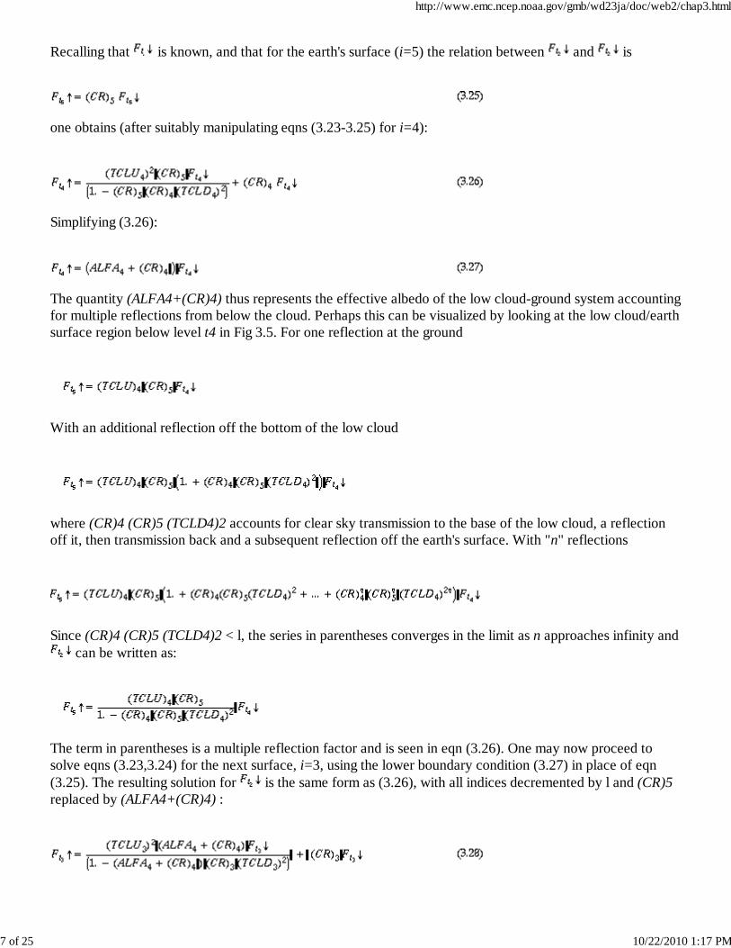
Recalling that is known, and that for the earth's surface (i=5) the relation between and is

one obtains (after suitably manipulating eqns (3.23-3.25) for i=4):

Simplifying (3.26):

The quantity (ALFA4+(CR)4) thus represents the effective albedo of the low cloud-ground system accountingfor multiple reflections from below the cloud. Perhaps this can be visualized by looking at the low cloud/earthsurface region below level t4 in Fig 3.5. For one reflection at the ground

With an additional reflection off the bottom of the low cloud

where (CR)4 (CR)5 (TCLD4)2 accounts for clear sky transmission to the base of the low cloud, a reflectionoff it, then transmission back and a subsequent reflection off the earth's surface. With "n" reflections

Since (CR)4 (CR)5 (TCLD4)2 < l, the series in parentheses converges in the limit as n approaches infinity and can be written as:

The term in parentheses is a multiple reflection factor and is seen in eqn (3.26). One may now proceed tosolve eqns (3.23,3.24) for the next surface, i=3, using the lower boundary condition (3.27) in place of eqn(3.25). The resulting solution for is the same form as (3.26), with all indices decremented by l and (CR)5replaced by (ALFA4+(CR)4) :


7 of 25 10/22/2010 1:17 PM

For the nth cloud, the ALFA term may be generalized (n=l-4):

where ALFA5=0.

The above procedure is repeated until the upward flux has been calculated for the top of the highest physicalcloud (i=2). Since is a clear sky flux, and is already known, eqns 3.30, 3.23, 3.24, 3.15-3.18, may beemployed to obtain upward and downward fluxes for all reflecting surfaces. Fluxes for a model level betweenthe clouds are easily obtained using clear-sky transmittances between the appropriate cloud top and bottomand the desired level. Finally, for cases where the cloud is more than one model layer thick (currently lowcloud), linear interpolation of transmission functions between cloud top and bottom produces values at modellevels inside the cloud. Application of eqn (3.7) results in identical shortwave heating rates for these internalmodel layers.

Surface Albedo Adjustment1.

Surface albedo is adjusted for the presence of snow at all land and sea-ice points. Poleward of approximately70_ latitude, surface albedo for snow covered land or sea ice is set to 0.75. Elsewhere the albedo, Rg is afunction of the background surface albedo, A0 (A0 = 0.5 for sea ice), and the snow depth, d (cm), as in eqn(3.31):

A zenith angle dependent surface albedo over open water is obtained from Payne's (l972) tabulated data.Payne accounts for the effect of atmospheric scattering and absorption on the surface albedo by tabulatingthe data as a function of atmospheric transmittance, TRANS, as well as zenith angle. The radiationparameterization uses a value of TRANS = .537 for all grid points, where TRANS=1. represents clearatmosphere.

Approximate Diurnal Cycle1.

Since the sun governs the diurnal cycle, shortwave (SW) processes are the most important to consider. Letting be the cosine of solar zenith angle at a point on the earth's surface, the "exact" shortwave flux, Fsw , at a

level in the atmosphere can be represented as:

where S is the solar constant, t is time, and Tr is the atmospheric transmissivity. Tr is a function of H2O, CO2,O3, other trace gases and aerosols (not considered here), and clouds. Holding these atmospheric profiles fixed( ), the SW flux integrated over a complete day is:


8 of 25 10/22/2010 1:17 PM

where the final equality exists because at night.

Ideally, one could simulate the diurnal cycle at a grid point by making radiation calculations each model timestep, thereby accounting for changes in zenith angle, H2O, temperature (for longwave computations) andclouds. This is computationally prohibitive however, so some approximations must be made. For example,one could either calculate the "less expensive" SW effects more frequently than longwave (LW) processes, orcalculate both SW and LW effects more frequently on a coarse subset of the grid and interpolate to the fullgrid. An alternative approximation, developed by Ellingson (U of Md) and Campana, for SW processes addslittle computational overhead (Campana, l986). A mean cosine of the solar zenith angle, , computed for eachmodel latitude as in eqn (3.34) of Manabe and Strickler (1964), and is used to calculate the SW fluxes at eachmodel "grid point".

Shortwave radiative fluxes are computed every 12 hours at all grid points using this mean cosine of the zenithangle, , as well as atmospheric transmissivities valid at those times (eqn (3.36)).

For the nondiurnal option these fluxes are fixed, but for the diurnal cycle option, grid point values of SWfluxes (and thus heating rates) are weighted by the exact cosine of the zenith angle, , at each forecastmodel time step, as in eqn (3.35):

where

and where represents grid point transmissivity at the beginning of a 12-hour interval. Though changes inH2O will occur during the 12-hour interval, a (reasonable) assumption is made that changes in are muchmore important than changes in water vapor profiles in determining SW fluxes. Integration of this SW fluxover 24 hours, again holding fixed, yields the same result as eqn (3.33)

Longwave Processes1.

Longwave radiative processes occur in a region of the electromagnetic spectrum distinct from shortwaveinfluences; at wavelengths greater than 4 ( =10-4 cm). In general, longwave effects are more difficult to


9 of 25 10/22/2010 1:17 PM

model than those in the shortwave part of the spectrum since both absorption and emission occur alongoptical paths and effects from all atmospheric layers must be included. The parameterization scheme, whichhas been developed by Fels and Schwarzkopf at GFDL, includes radiative effects of the ozone 9.6 band,the carbon dioxide 15 band, the water vapor band at 6.3 , the H2O "rotational " bands at wavelengthsgreater than 12 , and weak continuous H2O absorption in the 8 - 18 range. The 8 - 12 regioncontains virtually no specific H2O absorption bands and the weak continuous absorption is thought to be due,in part, to effects from strong H2O absorption outside this "window". Radiative effects from this "continuum"region occur primarily in the lower moist tropical atmosphere.

As in the parameterization of shortwave processes, the desired output from the longwave scheme are netradiative fluxes at all model levels which then are used to compute model layer heating rates (eqn (3.7)).Appropriate radiative transfer equations for the calculation of upward (F" ) and downward (F# ) longwaveflux at a specified atmospheric level, z, are (see Stephens, l984, p. 828):

where n is wavenumber (i. e., wavelength-1), Bn is the Planck function, zT is top of the atmosphere, and is the longwave transmission function between level and z . is defined over all zenith angles along

an optical path, du, in eqn (3.40):

where is cosine zenith angle and is the absorption coefficient (for an absorber concentration, u) whichvaries with pressure, p, and temperature, T, along the path from to z. The four integrals imbedded in eqns(3.38) - (3.40) make the numerical calculation of longwave effects quite expensive.

One can rewrite the radiative flux equations in a more convenient form by integrating eqns (3.38) - (3.39) byparts to obtain:

The net flux at level z, using eqns (3.41) - (3.42) is:

Changing vertical coordinate from z to pressure, p, noting that p=0 at z=zT and p=psfc at z=0, the net


10 of 25 10/22/2010 1:17 PM

longwave flux equation (3.44) is virtually identical to eqn (1) in Fels and Schwarzkopf (l975):

Computation of net flux at each model level requires the evaluation of integrals in eqn (3.40) and (3.44) for

1. zenith angle ( ),2. absorber optical path ( ),3. spectral interval ( ), and4. transmission from all levels ( ).

Fels and Schwarzkopf parameterize longwave processes using techniques designed to reduce thecomputational overhead inherent in these integrals, while, at the same time, retaining accuracy in thecalculations. The integral over zenith angle ( ) is removed by scaling the gaseous absorber path (i.e.,amount) by a diffusivity factor of 1.66. In this manner diffuse transmission from to p is represented, withlittle loss of accuracy (Rodgers and Walshaw, l966), as a beam of radiation along a path whose zenith angle,

, is approximately 53_.

The integral over optical path (du in eqn (3.40)) is difficult to compute because the absorption coefficientdepends upon pressure and temperature, both of which can change rapidly along du. There are techniqueswhich account for these inhomogeneous paths by adjusting pressure and path length to create a homogeneouspath having a mean absorption coefficient. Fels and Schwarzkopf use two methods for their water vaporcalculations. A simple scaling of the optical path by is used in their emissivity heating rate computations(discussed below), where =1013.25 mb. A more accurate scaling is the 2 parameter Curtis-Godsonapproximation where both pressure and absorber amount are adjusted to create the homogeneous path. Felsand Schwarzkopf employ this technique with the H2O random band model used for their exact heating ratecalculations (discussed below).

The integral over spectral interval ( in eqn. (3.44)) is quite difficult to calculate because the fine scale of theabsorption lines must be multiplied by the vertical derivative of the much smoother Planck function, Bn.Typically, methods are used which separate the longwave spectrum into spectral intervals small enough bothto consider the Planck function a constant and to produce transmission functions which are exponential innature (Stephens, l984). Though O3 and CO2 are evaluated as one band, H2O processes are complex enoughto require the smaller intervals. Using statistical properties for groups of absorption lines, an absorptioncoefficient can be defined as a function of the strengths, separations, and positions of the detailed linestructure within each spectral interval (or band). In "exact" calculations for water vapor, Fels andSchwarzkopf use the Rodgers and Walshaw (1966) random band model distribution of absorption lines andspectral intervals. In order to simplify the overlapping region of H2O and CO2 absorption (15 ), theRodgers and Walshaw bands 6,7,and 8 have been restructured to place all of the CO2 effects in band 7 (seetable 3.3, where, is mean line strength, is mean distance between absorption lines, and is (Lorenz) linewidth).

A less accurate but computationally more efficient alternative to the band model approximation for isthe emissivity approximation (see Stephens, l984; Paltridge and Platt, l976, p. 173). This treats the absorptionas a constant for all wavelengths within each spectral band and allows the integral over the entire spectrum tobe performed once, thus saving computer time. Fels and Schwarzkopf apply the emissivity approximation toeqn (3.44) and obtain the following flux equation (for H2O):


11 of 25 10/22/2010 1:17 PM

where are pre-calculated tables for temperature between 100K - 370K (every 10K) and for watervapor amount between 10-16 and 102 g/cm2 (180 values, equal spacing in ln u):

where n is the number of spectral intervals for H2O and is the transmission function for each band. Theintegral in eqn (3.45) is evaluated as

where j, j+1 refer to model levels and j+1/2, i+1/2 refer to model midlayers. For nearby layers, where , aprecomputed array, G3, is used to evaluate the integral:

Further details may be found in Fels and Schwarzkopf (l975).

One integral remains to be discussed - the integration over all atmospheric layers ( in eqn (3.44)). Fels andSchwarzkopf simplify this integration by separating the net radiative flux equation (3.44) into two terms(Green, l967):

1. Cooling to space (CTS), which is longwave emission from level p directly to space , and

2. Internal EXCHANGE between atmospheric levels, accounting for absorption and re-emission. Stephens(1984) notes that this process primarily occurs in "nearby" layers, because at greater distances its importancedrops with the exponential decrease of the transmission function.

In an isothermal atmosphere , and eqn (3.44) can be written as:

where Bn is the Planck function for each spectral interval, n, in the band model representation of thelongwave spectrum. The CTS approximation assumes that (3.48) can be used to calculate flux at all modellevels even though the atmosphere is not isothermal. The simplicity of this scheme can be seen in therepresentation of transmission functions in (3.44) and (3.48); the matrix calculation implied by in (3.44)is replaced by a function in (3.48) which depends only on absorber amount above level p. Of course, the CTSapproximation is not accurate enough by itself and the EXCHANGE term must be added.


12 of 25 10/22/2010 1:17 PM

Fels and Schwarzkopf treat the cooling-to-space and exchange calculations in different manners in order toobtain quite accurate results with a computationally efficient method. Recall from eqn (3.7) that the heatingrate, Q, is the vertical component of the radiative flux divergence. Computation of F(p) from eqn (3.44)produces a total heating rate, QTOTAL. Separation of the flux calculation into two terms can be used to obtaina CTS heating rate, QCTS (using eqn 3.48) and an exchange rate, QEXCHANGE (ie. the integral term in eqn3.44). Thus

Noting that the latter term is simply

Fels and Schwarzkopf find that the EXCHANGE is relatively insensitive to the method of calculation. Thusthey compute QEXCHANGE using the computationally more efficient emissivity ( ) method (3.45). Thecalculation of QCTS (in eqn (3.49) however is done more accurately - via either the Rodgers and Walshawrandom band (RB) model for H2O or accurate pre-calculated transmission functions for CO2. The "exact"CTS calculation adds relatively little overhead to the efficient computation for the EXCHANGE termbecause the former is a vector, not matrix, operation. The approximation to total longwave heating rate foreach model layer, using (3.49, 3.50), now becomes:

Heating rate calculations for both H2O and CO2 employ equation (3.51), however O3 processes arecalculated exactly, using eqn (3.44), for a one band model.

Water Vapor1.

For the "exact" CTS calculations (i.e., in eqn 3.51), the Rodgers and Walshaw random band model (Table3.3) is used. The transmission function, in eqn (3.48), is computed for each spectral interval as:

where , is absorber amount and (the diffusivity factor). More details can befound in Paltridge and Platt (l976), chapter 7. For the water vapor rotation bands (1-10), the Curtis-Godsonapproximation is employed to remove the effects of pressure on the transmission function along the opticalpath, du (see eqns (7.47) - (7.51) Paltridge and Platt, l976). An additional term is added to eqn (3.52) forbands 7-11, which partially covers the region of the water vapor continuum (band 21 completes thecontinuum region but is not included here, see section 3.4.2),

Note that the first term in (3.53) is zero for n=11, because A11=0. Eqn (3.53) is equivalent to a multiplicationof exponential transmission functions, where the pressure weighting accounts for pressure effects on the


13 of 25 10/22/2010 1:17 PM

continuum absorption coefficient along the optical path and

where (SK)n = 38.483, l6.288, 11.312, 7.428, 4.913 , for n=7,...,11. Equation (3.54) is from Roberts, et al.(l976) and accounts for the temperature, T, dependence of the absorption coefficient.

For the emissivity calculations ( in eqn 3.51), equations (3.45) - (3.47) are used, where G1, G2, G3are precomputed in tabular form using the Rogers and Walshaw parameters in Table 3.3 for strong absorptionline transmission (see Paltridge and Platt, l976, eqn 7.38):

Water vapor amount scaled by is used during the table "look-up" for G1, G2, and G3. Water vaporrotational band 7 for these emissivity calculations is handled in the CO2 overlap (section 3.4.3). Thecontribution due to lines in bands 8-11 and 21 is neglected in eqn (3.55), however the effect of lines in bands8-11 is included in the "exact" CTS computation (eqn 3.53). For the emissivity calculations, the continuumeffects in bands 8-11 are included as a one broad band calculation and added to and , after the G1,G2, G3 table "look-up". Transmission in this one band continuum is:

where 8.6658 is a frequency weighted mean of the (SK)n (n=8-11) in eqn (3.54). Emissivity calculations forthe continuum in band 7 are included in the CO2 overlap (section 3.4.3).

Ozone1.

Ozone processes are not split into CTS and EXCHANGE terms. Parameterization of O3 effects is "exact"using the one interval random band model of Rodgers (l968). The transmission function in eqn (3.44) iscomputed for band 21 (table 3.3) as:

where p is pressure in units of atmospheres, =1.66, and and are absorber amounts. Using Rodgersnotation


14 of 25 10/22/2010 1:17 PM

with =.28 cm-1, =.1 cm-1, k=208. cm g-1. The overlap with water vapor continuum (thus treated"exactly") is included as the last term in eqn (3.56) where

Carbon Dioxide1.

Transmission functions for carbon dioxide are precomputed using techniques described by Fels andSchwarzkopf (l981), as updated in Schwarzkopf and Fels (l985). Detailed "line by line" procedures are usedto obtain CO2 (330ppmv) transmission functions and their first and second temperature derivatives for theforecast model's vertical coordinate. Standard atmosphere temperature profiles and two specified surfacepressures (1013.25 mb, 810.6 mb) are used. The CO2 transmission and derivatives are available in block data,BD2. Interpolation of the transmission, , and its derivatives to the vertical structure of each model grid pointis simply:

where and represent the two model profiles available in block data. The interpolation of transmissionfunctions to the temperature profile of the particular grid point is made from a second order expansion below:

where is from (3.57) and (eqn (33) in Fels and Schwarzkopf (1981)) is

Numerical experimentation shows that

where po=30 mb and p is model level pressure using psfc=1013.25 mb. The function G(p) is precomputed andresides in block data, BD2 (GTEMP).

A temperature correction to in (3.58) is necessary because the spectral interval (band 7) is not really narrowenough to consider the Planck function a constant. The final transmission function, is (eqn (7) inSchwarzkopf and Fels (l985)):


15 of 25 10/22/2010 1:17 PM

where

For the "exact" CTS heating rate calculation, in eqn (3.51), CO2 transmission is multiplied by the H2Oband transmission (eqn 3.53)) to account for absorption overlap. For the emissivity EXCHANGE heating ratecalculation, , in eqn (3.51), a one band version of eqn (3.44) is used. Overlapping H2Otransmission is computed as (see eqn (3.54) and (3.55)):

where C7 is defined in eqn (3.54), and the strong line approximation is used for H2O band 7.

Clouds1.

Three types of stratiform cloud are allowed (section 3.2.3) and for longwave processes all are consideredblackbodies. Model levels are vertical boundaries for the clouds; however, unlike the shortwaveparameterization, the bounding surfaces are considered to be in clear sky (Fig 3.6a). The longwave radiativeflux at a particular level, p, is weighted by the percentage of clear sky in the optical paths from allatmospheric levels to level p. When more than one cloud type exists in a path, the clouds are randomlyoverlapped (Fig 3.6b).

In the case of thick (i.e., greater than one model layer) low cloud, longwave processes result in strong coolingin the upper cloud layer and much less cooling in the lower cloud layer. This produces a strong destabilizingeffect, which could be harmful when used with the fixed zonal mean cloud climatology. An adjustment ismade to the vertical gradient of longwave flux in the thick cloud (a smoothing!) so that it is constant for thecloudy part of the column. For completely overcast low cloud situations (i.e., cloud fraction =1), the resultingmodel layer longwave heating rates within the cloud will be identical.

Adjustment to the Surface Downward Flux1.

When the approximate diurnal cycle is used for SW processes (section 3.3.6), changes to model temperatureand H2O profiles in the lower atmosphere can be large. Since longwave heating rates are held fixed for each12-hour interval, they could be seriously in error during parts of the model-day. There is, however, anadjustment to downward LW flux at the earth's surface ( ), for these large diurnal changes, whichreduces the potential "12-hour shock" to the land surface temperature. Changes to are computed byassuming that the ratio is constant at each forecast model time step, where T1 is lowest modellayer temperature. Thus when T1 increases (decreases) during the forecast, an estimate of the increase(decrease) of is obtained. The downward longwave flux is computed as in eqn (3.62), where ( )odenotes values at the beginning of each 12-hour radiation computation interval and ( )n are values at each


16 of 25 10/22/2010 1:17 PM

model time-step.

Table 3.1

Discrete probability distribution,, of water vapor absorption coefficients, kn, for N=9 subintervals of the solarspectrum (see Lacis and Hansen (l974), table 1)

Table 3.2

Shortwave radiative properties of clouds for the 9 subintervals of the solar spectrum

Table 3.3

Water vapor band parameters used for exact CTS calculations. Bands (7-11,21) are H2O continuum and band21 is for exact O3 computation, but neither is part of Rodgers and Walshaw (1966) model. H2O rotationbands (1-10) and 6.3 bands (12-20) from Rodgers and Walshaw. Adjustments made to bands 6-8 so thatCO2 effects lie entirely within band 7.


17 of 25 10/22/2010 1:17 PM

Campana, K. A., l986: "An Approximation to the Diurnal Cycle for use in NMC's Medium-Range ForecastModel", Medium-Range Modeling Br. Note, unpublished.

Fels, S. B. and M. D. Schwarzkopf, l975: "The Simplified Exchange Approximation - A New Method forRadiative Transfer Calculations", J. of Atmos. Sci., pp.1475-1488.

Fels, S. B. and M. D. Schwarzkopf, l981: "An Efficient, Accurate Algorithm for Calculating CO2 15 BandCooling Rates", J. of Geophys. Res., pp. 1205-1232.


18 of 25 10/22/2010 1:17 PM

Green, J. S. A, l967: "Division of Radiative Streams into Internal Transfer and Cooling to Space", Quart. J. ofRoy. Met. Soc., pp. 371-372.

Hering, W. S. and T. R. Borden, Jr., l965: "Mean Distribution of Ozone Density over North America,l963-l964", Environmental Research Papers, Report 162 USAF Cambridge Research Laboratory.

Lacis, A. A. and J. E. Hansen, l974: "A Parameterization for the Absorption of Solar Radiation in the Earth'sAtmosphere", J. of Atmos. Sci., pp. 118-133.

London, J., l962: "Mesospheric Dynamics, 3, the Distribution of Total Ozone in the Northern Hemisphere,Final Report", Dept. of Meteorology/Oceanography, New York University.

Manabe, S. and R. F. Strickler, l964: "Thermal Equilibrium of an Atmosphere with a Convective Adjustment",J. of Atmos. Sci., pp. 361-385.

Matthews, E., l985: "Atlas of Archived Vegetation, Landuse, and Seasonal Albedo Data Sets", NASATechnical Memorandum 86199, Goddard Institute for Space Studies, New York.

Paltridge, G. W. and C. M. R. Platt, l976: "Radiative Processes in Meteorology and Climatology, ElsevierScientific Publishing Company.

Payne, R. E., l972: "Albedo of the Sea Surface", J. of Atmos. Sci., pp. 959-970.

Roberts, R., J. Selby, and L. Biberman, l976: "Infrared Continuum Absorption by Atmospheric Water Vaporin the 8-12 Window", Applied Optics, pp. 2085-2090.

Rodgers, C. D. and C. D. Walshaw, l966: "The Computation of Infrared Cooling Rate in PlanetaryAtmospheres", Quart. J. of Roy. Met. Soc., pp. 67-92.

Rodgers, C. D., l967: "The Radiative Heat Budget of the Troposphere and Lower Stratosphere", Report No.A2, Planetary Circulations Project, Dept. of Meteorology, M. I. T.

Rodgers, C. D., l968: "Some Extensions and Applications of the New Random Model for Molecular BandTransmission", Quart. J. of Roy. Met. Soc., pp. 99-102.

Sasamori, T., J. London and D. Hoyt, l972: "Radiation Budget of the Southern Hemisphere", MeteorologicalMonagraphs, vol. 13, number 35, pp. 9-23.

Schwarzkopf, M. D. and S. B. Fels, l985: "Improvements to the Algorithm for Computing CO2Transmissivities and Cooling Rates", J. of Geophys. Res., pp. 10541-10550.

Stephens, G. L, l984: "The Parameterization of Radiation for Numerical Weather Prediction and ClimateModels," Mon. Wea. Rev., pp. 826-867.

Telegadas, K and J. London, l954: "A Physical Model of the Northern Hemisphere Troposphere for Winterand Summer," Sci. Rpt. 1, Research Division, College of Engineering New York University, 55 pp.


19 of 25 10/22/2010 1:17 PM

Fig 3.1 Schematic of radiation calculations, with subroutine names.


20 of 25 10/22/2010 1:17 PM

Fig 3.2 Seasonal zonal mean ozone (parts per million) in upper nine layers of the 18 layer model. Mean layerpressure (mb) for surface pressure=1000 mb. Contour interval = 0.5 ppm.


21 of 25 10/22/2010 1:17 PM

Fig 3.3 Seasonal zonal mean cloud fraction for high, middle, and low cloud climatology. (a) Northernhemisphere winter. (b) Northern hemisphere spring. Values hemispherically flipped for opposite season.


22 of 25 10/22/2010 1:17 PM

Fig 3.4 Seasonal cloud thickness in model sigma layers (surface pressure = 1000 mb). High and middle cloudsare one layer thick. (a) Northern hemisphere winter. (b) Northern hemisphere spring. Data hemisphericallyflipped for opposite season.


23 of 25 10/22/2010 1:17 PM

Fig 3.5 Multiple reflections for the short wave cloud calculation. Subscripts for TCLU and TCLD are invertedin subroutine SWR983 ; i.e. TCLU4 becomes TCLU1 , etc...


24 of 25 10/22/2010 1:17 PM

Fig 3.6 Model clouds. (a) Schematic representation of cloud bounding surfaces for short wave (SW) and longwave (LW) processes. (b) Cloud overlap, where H, M, L are cloud fraction for high, middle, and low cloudrespectively.


25 of 25 10/22/2010 1:17 PM

1. radiation · latitude climatology (fig 3.2) has been constructed from hering and borden (l965)...

Documents