1. Introduction: why molecular astrophysics?

1.1 Motivation for studying molecules 1.1.1 Widespread occurrence of molecules A wide variety of molecules are found in a wide variety of astrophysical environments:

• Interstellar medium • Circumstellar outflows • Cometary comae • Accretion disks • High-z galaxies

(Also, stellar and planetary atmospheres, not considered in this course.)

List of ~ 100 molecules detected in the ISM: some familiar, some very exotic (V1.1) 1.1.2 Importance of molecules as probes a) As a probe of excitation conditions: thanks to the rich spectrum of rotational, vibrational and electronic transitions Examples: CN as a probe of the CMB (V1.2) High-J CO as a probe of shocked

regions (V1.3) H2 fluorescence as a probe of UV

continuum radiation (V1.4)

b) As a chemical probe: Examples:

Cosmic ray ionization rate (V1.5) Water in NGC 4258 disk (V1.6) c) As a kinematic probe: thanks to the high brightness temperature of maser spots Example: Water masers in Galactic sources (V1.7) d) As a probe of isotopic abundances: thanks to the large isotopic shift Example: Galactic 12C/13C ratio (V1.8)

e) As a magnetic probe: thanks to the Zeeman shift Example: OH masers, H2O masers 1.1.3 Importance of molecules as coolants

i. in gas in galaxies (V1.9) ii. in pre-galactic gas (V1.10)

1.2 Observations of molecules 1.2.1 Electronic transitions (UV/Visible lines) First known interstellar molecules detected by visible wavelength absorption line spectroscopy towards background stars: CH, CH+, and CN In UV, also observe absorption by: CO, OH, H2 , HD (Copernicus, IUE, HST, HUT, FUSE) High spectral resolution => rotational spectrum

In certain circumstances (especially reflection nebulae and cometary comae), we also see emission. Emission in electronic transitions is never collisionally-excited: molecules cannot survive at temperatures that would be required. Emission is pumping fluorescently by interstellar (or solar) UV radiation. 1.2.2 Vibrational transitions (Visible/Infrared) Fundamental vibrational modes often observed in 2 - 7 micron region. Can be observed in absorption toward sources of higher extinction.

Examples: CO, H2O, H2 (even though it has no dipole moment). Emission is also observed, particularly from H2 in the 2 micron region. Origin can either be collisional excitation (in T ~ 2000 K gas) or fluorescent pumping. Use line ratios as a discriminant. 1.2.3 Rotational transitions (Radio/Far-Infrared) (also inversion, hyperfine transitions) Before 1964, only three known molecules. Enormous progress in molecular astrophysics has resulted from low noise radio receivers operating at ever higher frequencies.

See a forest of rotational lines (V1.11) Low-frequency: low-lying transitions of heavy molecules Examples: CO J=1-0 115 GHz CO J=2-1 230 GHz High-frequency: low-lying transitions of hydrides, or high-lying transitions of heavy molecules Examples: HCl J=1-0 626 GHz HF J=2-1 2463 GHz Many high-J CO lines Observations at submillimeter (300-1000 micron) and far-infrared (30-300 micron) wavelengths are often significantly affected by atmospheric absorption

Submm/Far-IR Instruments:

• CSO and JCMT (10 and 15m telescopes in Mauna Kea)

• ASTRO (1.8m at South Pole) • KAO (0.91m in C-141 at 45,000 ft) • Balloons (up to 130,000 ft) • Infrared Space Observatory

(0.6m FIR telescope in space) • SWAS (0.6m submm. telescope in space) • SOFIA (Boeing 747 at 45,000 ft) • SMA and ALMA (submm. arrays) • FIRST (4m in space)

2. Diffuse Molecular Clouds 2.1 Overview Cold dense clouds make up most of the mass of the ISM.

Typical temperature ~ 100 K Typical density ~ 100 - 1000 cm-3 Typical size ~ 1 - few pc AV ~ 3.1 E(B-V) ~ 0.59 NH / 1021 cm-2

in range 0.3 - 2

Clouds with column density greater than ~ 5 x 1020 cm-2 show a significant molecular content (V2.1, V2.2 from Savage et al. 1977)

2.2 The molecular hydrogen problem Seek to explain formation of H2 and non-linear dependence on column density 2.2.1 Formation and destruction of H2 H2 has a dissociation energy of 4.48 eV, so at 100 K (equivalent to ~ 0.01 eV) in thermal equilibrium the ISM would be all molecular. But, interstellar H2 is destroyed by photodissociation caused by the UV background.

The photodissociation rate due the mean interstellar radiation field (Draine 1978) is n(H2) ζH2 per unit volume.

For typical interstellar radiation field, ζH2 = 5 x 10-11 s-1 in the limit of no shielding

H2 formation via gas-phase reactions: possible mechanisms

1) Three-body formation H + H + H à H2 + H Important only at high density

(nH > 1015 cm-3)

2) Radiative association H(1s) + H(2s,2p) à H2 + hν

Slow, and requires H in n=2

3) Formation via H- H + e à H- + hν H- + H à H2 + e Slow, and requires electrons (d) Formation via H2

+ H + H+ à H2

+ + hν H2

+ + H à H2 + H+ Slow, and requires protons In cold neutral clouds, none of these processes is nearly fast enough to account for the observed abundance of H2.

Only viable mechanism: GRAIN CATALYSIS Picture (from Shu’s The Physical Universe)

Maximum rate per unit volume ~ ½ n(H) Σd nH <vth> = kf n(H) nH

Mean thermal velocity

Grain surface area per H nucleus ~ 10-21 cm2

Maximum kf ~ 7 x 10-17 T2

1/2 cm3 s-1 To account for the observations, kf ~ 3 x 10-17 T2

1/2 cm3 s-1 is required, so the process must be fairly efficient. In equilibrium (for nH = 100 cm-3, T=100K, Mean IS UV field), ζH2 n(H2) = kf n(H) nH è n(H2)/n(H) = kf nH/ζH2 = 6 x 10-5

2.2.2 Destruction of H2 Many diffuse clouds with Av < 1 show n(H2)/n(H) > 1

Explanation: H2 self-shielding Outer skin shields interior from photodissociation Outer skin of H with trace of H2 H2

Self-shielding is very effective because H2 photodissociation occurs following line absorption. Once the lines get optically-thick, the photodissociation rate starts to drop rapidly.

Picture (from van Dishoeck 1988 review)

Derive dependences on N(H2) in one-line approximation Rate, ζ, roughly proportional to dW/dN(H2), where W is the line equivalent width a) Small N(H2): ζ = constant b) Intermediate N(H2):

ζ ∝ N(H2)-1 [ ln (N(H2)/N0) ] -1/2 c) Large N(H2): ζ ∝ N(H2)-1/2 d) Very large N(H2): ζ ∝ exp[-c N(H2)] due to line overlap and dust

2.2.3 Theoretical models for molecular fraction Simple isodensity slab models IUV W(N(H2)) proportional to nH N(H) ---> non-linear growth (V2.4) Three Dimensional Models Use 26-ray approximation. Compare prediction with excess I100/N(H) ratio (V2.5-2.9) Ref: Spaans and Neufeld (1997)

2.2.4 H2 level populations Need to solve equations of statistical equilibrium for level populations. Let fi be the fraction of H2 in state i 0 = dfi/dt = ∑ fj (Aji + Cji + Rji)

− fi ∑ (Aij + Cij + Rij) where Aij, Rij, and Cij are the rates of transitions from i to j that result from spontaneous radiative decay, pumping via the Lyman and Werner bands, and collisional excitation. This is a matrix equation of the form df/dt = M f

Two methods of solution: 1) integrate in time until f converges

(NB: stiff equations) 2) solve M f = 0 subject to

(1 1 1 1 .... 1) . f = 1 Compare with observations of 1) fluorescent emission at UV, IR and visible wavelengths e.g. Neufeld and Spaans (1996) (V2.10) 2) absorption from various rotational states J = 0 through 5 Typical result: J = 0, 1, 2 populated by collisions; higher J populated by pumping (V2.11)

2.3 Gas-phase chemistry Ref: van Dishoeck (1997) Elemental abundances: (V2.12) 2.31 Observed molecules in diffuse clouds: Optical absorption: CH, CH+, CN UV absorption: H2, HD, CO, OH, HCl? (Federman et al. 1995) Infrared absorption: C2 Radio emission: CS, CO, CN Radio absorption: NH3, H2CO, HNC, C2H, C3H2, HCN, HCO+, SO, H2S (Lucas and Liszt 1997)

2.32 Deuterium chemistry: proof of the importance of gas phase chemistry. If HD were formed on dust grains, like H2, would expect: n(HD)/nH = k n(D) / ζ0 ~ 10-9 (if n(D)/n(H) ~ few x 10-5) Typical value in substantially molecular gas: 10-6 ==> formed by exchange reaction D+ + H2 <---> HD + H+ Tends to equilibrate towards n(HD)/n(H2) = nD/nH ~ 10-5

Why reaction with D+? Because reaction with D is too slow. Where does D+ come from? Cosmic ray ionization: CR ==> H ----> H+ + e H+ + D <---> H + D+ Required c.r. ionization rate for nD/nH ~ 10-5: ζcr = several times 10-17 s-1 So, observations of HD ==> importance of gas phase chemistry importance of cosmic ray ionization

2.33 Types of reactions Endothermic versus exothermic: plot E versus “reaction coordinate” Molecular processes Name Example “Typical” rate

coeff (cm3 s-1) Ion-neutral H2 + D+ --> HD + H+ 10-10 - 10-9 Neutral-neutral H2 + D --> HD + H 10-11 - 10-9

x exp (-EA/kT) Grain catalysis gr-H + H --> gr + H2 3 x 10-17 Photodissociation H2 + hν --> H + H 10-10 (units = s-1) Cosmic ray CR: H2 --> H2

+ + e few x 10-17 ionization (units = s-1) Dissociative H3O+ + e --> OH + H + H few x 10-7 recombination Radiative C+ + H2 --> CH2

+ + hν 10-15 association

2.34 Oxygen chemistry 2.341 Formation of OH Simplest oxygen-bearing molecule is OH. OH is less strongly bound than H2, so the obvious reaction O + H2 --> OH + H is endothermic. Reaction barrier is EA/k ~ 3000 K, so important only at high temperature. (Actually, can be important in mainly molecular gas at T > 300 K, but not in 100 K diffuse clouds)

Like deuterium chemistry, oxygen chemistry is initiated by cosmic rays, The OH abundance, like the HD abundance, probes the cosmic ray ionization rate. CR: H --> H+ + e H+ + O --> H + O+ (EA/k ~ 230 K) Then O+ + H2 --> OH+ + H (exothermic, no barrier) Further reactions with H2: OH+ --> H2O+ --> H3O+

[If a molecular ion can react rapidly with H2 it will: kin n(H2) > kdr n(e) ] H3O+ does not react with H2, so it is most likely to undergo dissociative recombination: H3O+ + e --> OH + H + H fOH OH + H2 or H2O + H fH2O or O + H + H2 fO O + H + H + H

Controversy over branching ratio. Two recent experiments: 1) Nigel Adams’ group:

5% water, 65% OH, 30% O 2) Danish group:

25% water, 74% OH, 1.3% O Search for water using HST in cloud of Av = 2.5 mag in front of HD 154368 (2 lines around 1240 Angstrom; see Spaans et al. 1998, ApJ, 503, 780) N(OH) = 1.4 x 1014 cm-2 N(H2O) < 0.9 x 1013 cm-2 (3 σ limit) è N(H2O)/N(OH) < 0.07

Plot from Marco Spaans diffuse cloud code (vary f and ζcr): results consistent with Adams’ small value for fH2O However, recent submillimeter/radio absorption line studies obtained a different result toward the W51 (HII region/dust continuum source) - see Neufeld et al. 2002, 580, 278 N(OH) = 8 x 1013 cm-2 N(H2O) = 2.5 x 1013 cm-2 è N(H2O)/N(OH) ~ 0.3

If OH and H2O are formed exclusively by dissociative recombination of H3O+ and are destroyed exclusively by photodissociation, then we expect a ratio

where

ζH2O = 3.5 × 10-10G0 exp(-1.7AV) s-1 ζOH = 5.1 × 10-10G0 exp(-1.8AV) s-1 are the photodissociation rates for OH

and H2O (Roberge et al. 1991, Here, G0 is the strength of the interstellar radiation field relative to the “mean value” (Draine 1978). Yields N(H2O)/N(OH) = 0.17 and 0.05 for Adams’ and Danish groups respectively.

More detailed theoretical calculations confirm the “toy model” results given above, and the W51 results would seem to imply a large value of fH2O

(see figure) However, fH2O is determined by quantum mechanics, of course – it cannot vary from cloud to cloud. Different values of N(H2O)/N(OH) in different clouds must imply some additional formation (or destruction process) Possibilities under consideration:

• Neutral-neutral reactions in an enhanced temperature component (see figure from Neufeld et al. 2002)

• Grain surface reaction to produce H2O

High-T calculations for 100, 300, 400, 450, 500, 550, 600, 700, 800,

and 1500 K.

2.342 Reactions of OH 1) OH destruction is dominated by UV photodissociation. 2) OH is an important intermediary in the production of CO and HCO+ through reactions with C

OH + C --> CO + H (believed to be rapid at low temperature)

and especially with C+

OH + C+ --> CO+ + H CO+ + H --> CO + H+

CO+ + H2 --> HCO+ + H HCO+ + e --> CO + H

2.35 Carbon chemistry 2.351 Formation & destruction of CH Crucial difference between O and C: Ionization potential of C < 13.6eV => not shielded by H C+ is therefore the dominant form of C: cosmic ray ionization irrelevant. But 2nd crucial difference:

C+ + H2 à CH+ + H is endothermic Formation of carbon hydrides is probably initiated by a (slow) radiative association reaction (upper limit on rate from laboratory measurements) C+ + H2 --> CH2

+ + hν

Then CH2+ + H2 --> CH3

++ H CH3

+ + e --> CH, CH2 CH destroyed primarily by UV photodissociation For reasonable values of the radiative association rate, models match the observed CH abundance 2.352 Other carbon molecules CO and HCO+ Formed primarily by reaction of OH with C+ (see section 2.343 above) CO photodissociation follows line absorption like H2

==> self-shielding and shielding by H2.

Models tend to underpredict CO abundance (assume too much radiation below 1000 Angstrom?) CN, C2, and C2H More complex formation mechanisms Models tend to underpredict CN 2.353 The CH+ problem The CH+ abundance, however, is seriously underpredicted (by a factor ~ 100). Problem: C+ + H2 --> CH+ + H is endothermic

Alternate routes are inefficient (photoionization of CH, reaction of C with H3

+) Maybe this is telling us something interesting: some fraction of gas is warmed so that the energy barrier is overcome? Suggested as evidence for shock heating. Problem: models with warm gas may overproduce OH and J > 3 H2. Possible solution: MHD shocks with ion-neutral drift could preferentially drive endothermic ion-neutral reactions.

2.354 Large molecules/small grains Observational evidence for polycyclic aromatic hydrocarbons: IRAS cirrus observations, infrared emission bands, extended red emission Consequences for the chemistry: ionization level reduced PAH + X+ ---> PAH+ + X (charge transfer) PAH+ + e ---> PAH* (rapid recombination) PAH* ---> PAH + hν

3. Dense molecular clouds 3.1 Astrophysical overview By convention (and somewhat arbitrarily), dense clouds are taken here to mean molecular clouds of Av > 2. Note that column density rather than physical density defines the distinction between diffuse and dense molecular clouds.

3.1.1 Translucent clouds have Av in the range 2 - 5 mag. • Observable by means of both visible/UV

absorption lines and millimeter wave emission lines. Emission lines ==> mapping, but column densities more model-dependent.

• Higher molecular abundances than

diffuse clouds, but UV photodissociation still important.

• Somewhat higher densities (several

hundred cm-3) as self-gravity starts to be important.

Example: cloud in front of HD 169454 (see van Dishoeck review article).

3.12 Dark clouds • Readily apparent in star maps (V3.1). • nH ~ 103 cm-3; Av ~ 10 ==> interstellar

UV field negligible • Heated and ionized mainly by cosmic

rays: T ~ 10 K, fractional ionization ~ 10-7

Example: Taurus Molecular Cloud 1 (TMC-1)

3.13 Molecular cloud cores • Dense (nH > 104 cm-3), self-

gravitating clumps of size ~ 0.1 pc within dense molecular clouds.

• Stand out in observations of

molecular lines with high critical density (e.g. NH3 transitions).

• Sites of star formation

3.14 Effect of star formation on molecular clouds (to be considered further in Sect. 4) • Protostars: central source of L = 10 -

105 solar luminosities heats cloud core from inside ==> “hot core” with warm gas up to 1000 K (V3.2, V3.3, V3.4 from Doty and Neufeld 1997 models)

Example: Orion IRC 2

• Bipolar outflows: mass loss in

disk/stellar wind (up to 200 km/s) creates shocks at interface with ambient cloud material

Example: Orion, NGC 2071 (V3.5, V3.6)

• Young massive stars: O or B stars ==> very high UV field (IUV up to 105)

Example: Kleinman-Low nebula in Orion

3.2 Chemistry of cold, quiescent dense clouds. Key differences from diffuse cloud case: 1) Temperature lower (except due to effects described in 3.14)

==> some reactions much slower, e.g. O + H+ --> O+ + H

2) Interstellar UV field weak or absent ==> ionization much lower (very little C+)

photodissociation rates much smaller

3.21 Steady state models 3.211 Overview Chemistry driven by cosmic rays. Formation of molecules typically involves the key molecule: H3

+ H3

+ is produced in the sequence: CR: H2 ---> H2

+ + e H2

+ + H2 ---> H3+ + H

H3

+ can then transfer a proton to any of C, O, S, Si, Cl (but not N or F) initiating the ion-neutral chemistry.

Nitrogen chemistry is initiated by the unusual reaction N + H3

+ ---> NH2+ + H

(May alleviate the NH3 problem described by Millar.) Fluorine might react with H3

+ in an analogous reaction, but fluorine is unique in reacting exothermically with H2 to form HF (only interstellar hydride that is more strongly bound than H2) F + H2 ---> HF + H

Laboratory measurements show that the F + H2 reaction has a barrier EA/k ~ 500 K. At temperatures below ~ 30 K, reaction with water (no barrier) dominates F + H2O ---> HF + OH Models ==> HF dominant reservoir of fluorine over a wide range of conditions. (HF first observed with ISO) Destruction of many molecules also often involves cosmic rays. Cosmic rays penetrate deep into dense clouds and dense cloud cores.

Cosmic rays create a local UV field because the 30eV secondary electrons excite Lyman and Werner band transitions. Intensity ~ N(H2)τ =1 ζcr hν/4π Typical photodissociation rate

~ 4π x intensity/hν . σ ~ N(H2)τ=1 σ ζ cr ~ 1021 10-17 10-17 s-1 ~ 10-13 s-1 The internal UV field is larger than interstellar radiation field if extinction factor greater than about 1000 (corresponding to 7.5 mag)

3.212 Model Calculations There are typically many routes to the formation of a specific model, so complex numerical calculations are needed. The chemical rate equations have the form

dY/dt = F(Y),

where F is a non-linear function of Y with a large number of terms of the form k Yi Yj In steady-state, we look for a solution to 0 = dY/dt, subject to a series of constraints on the total number of nuclei for each element (we consider chemical reactions not nuclear reactions!)

Most robust method of solution is to integrate the time-dependent equations until dY/dt reaches zero. Two important differences with the level-population rate equations.

1) Chemical timescale can be long relative to astronomical timescales, so time-dependence may be important 2) Rate equations are non-linear ==> no guarantee that there is a unique steady-state solution (c.f. 3.23 below)

3.213 Model Results

Several complex models involving thousands of reactions and hundreds of species have been constructed. The most complete reaction set is the UMIST compilation, available in computer-readable form. The most noteworthy shortcomings of steady-state models is that they predict too little C and too much O2.

Carbon I Models predict that CI will be abundant only in an interface zone at Av ~ 4 (V3.7) Observations show widespread and spatially extended emission in the 609 micron fine structure line of CI (V3.8) Molecular oxygen Models predict large O2 abundances (> 10-5) produced by O + OH ---> O2 + H

Searches for 16O18O emission or 16O2 emission/absorption in redshifted galaxies had placed upper limits as small as 10-6 for some sources. SWAS limits now imply O2 abundance < few x 10-7 in many sources Suggested solutions: 1) Internal sources of UV radiation: violated by bolometric luminosity of several sources 2) Carbon/oxygen ratio > 1: astrophysically implausible unless oxygen highly depleted as water ice. Observed strength of IR water ice features argues against high depletion (but could be selection effect)

Would also explain low water vapor abundances derived by SWAS for cold quiescent clouds 3) Bistability (section 3.22) 4) Time-dependent chemistry (section 3.23)

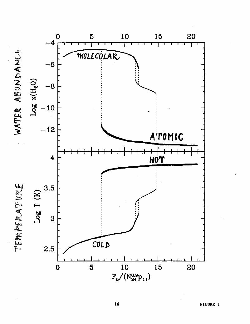
3.22 Bistable solutions Non-linear rate equations ==> possibility of multiple solutions. Le Bourlot et al. found that if the sulphur depletion is 10 or greater, two stable solutions can exist over a limited range (~ factor 4) of densities and temperatures (V3.9, V3.10). The higher ionization phase has larger CI and lower O2 abundances than the lower ionization phase solution.

3.23 Time dependent models Timescale for H2 formation ~ 1/(k nH) ~ 1 Myr (103 cm-3/nH)

Timescale for ion-molecule chemistry

~ 0.1 Myr (V3.11) Time dependence important if molecules destroyed by shocks or brought by turbulence to cloud surface on shorter timescales.

3.24 Deuterium fractionation At low temperatures, thermodynamics can significantly favor deuterated species so that n(MD)/n(MH) >> D/H. Effectiveness of ion-neutral exchange reactions in fractionating deuterium probes the cosmic ray ionization rate.

4. Regions of star-formation The star-formation process itself has a feedback effect on the surrounding molecular gas, causing regions of active star-formation to be profoundly different from cold, quiescent clouds. 4.1 Cloud cores with embedded protostars Protostars are sources of substantial luminosity which heat the surrounding molecular gas.

4.11 Physical conditions Start by considering the physical conditions in a star-forming cloud core. 4.111 Density Hydrostatic equilibrium Molecular cloud cores have substantial self-gravity, so they are centrally-condensed. Consider equations of hydrostatic equilibrium for the simplified case of an isothermal, non-magnetic, spherically symmetric core (isothermal sound speed a = constant). Equation of state: p = ρa2

Hydrostatic equilibrium:

dP/dR = -GM(<R)ρ/R2 Mass equation:

dM(<R)/dR = 4πR2ρ Boundary conditions:

M(<R) = 0 at R = 0 P = Pext at R = Rext The nature of the solution depends upon the outer boundary condition: the entire family of solutions is referred to as the Bonner-Ebert spheres.

Simplest cases are (1) the singular isothermal sphere (SIS), obtained if Pext Rext

2 = a4/2πG (minimum value for which a solution can be obtained) ρ = a2/2πG R-2 M=2a2/G R P=a4/2πG R-2 (2) the isobaric sphere, obtained in limit Pext Rext 2 >> a4/2πG (negligible self-gravity) ρ = a2 Pext M= 4πR3 a2 Pext/3 P = Pext

The general solution has ρ approximately proportional to R-2 in the outer regions but leveling off to some maximum value at the center (V4.1) Inside-out collapse Key point: not all solutions to the Bonner-Ebert problem are stable equilibria. In particular, the solution is unstable if Pext Rext

2 < 1.5 a4/2πG. The SIS solution is therefore unstable. Shu (1977) showed that it is subject to an “inside-out” collapse.

Obtained self-similar solution, with expansion wave propagating out at speed a

Outside R = a t, we have the (unperturbed) SIS solution, r ~ R-2. Inside R = a t, we have r approximately proportional to R-1.5 and an infall velocity ~ (a3 t / R)0.5 The mass accretion rate is dM/dt = 0.975 a3/G ~ 1.3 10-6 (a/0.17 km/s)3 Msolar yr-1

Observational constraints Density profile can be deduced

(1) from measurements of the dust continuum spectrum, and (2) from high-resolution observations of the spatial distribution of H2CO emission

Typical result:

d log ρ/ d log R = -1 to -2 (V4.2)

4.112 Temperature Absent any central source of luminosity, the temperature equilibrates to ~ 10 K, with cosmic ray heating in balance with CO cooling. However, protostars are substantial sources of luminosity:

Stellar luminosity (nuclear reactions) up to 105 Lsolar Accretion luminosity ~ G M (dM/dt) / R* ~ 25 (M/Msolar) (Rsolar/R) x (dM/dt /10-6 Msolar yr-1) Lsolar

Dust temperature obtained by solving the continuum radiative transfer problem. If temperature exceeds ~ 1000-2000 K, grains vaporize ==> “opacity gap” at center of core. Typical temperature profile:

d log T / d log R ~ -0.5 Gas temperature coupled to dust temperature in inner regions but falls below in outer regions. (V4.3 - 4.5)

4.12 Chemistry In inner regions, gas temperature can significantly exceed the 100 K temperatures considered previously in diffuse clouds. Two important effects: high-temperature reactions in the gas-phase, and grain mantle vaporization. 4.121 High temperature reactions Inner regions of “hot cores” can contain gas at temperatures as large as 1000 K. In small volume, at least, neutral-neutral reactions with large EA can be important.

Expect profound effect on oxygen chemistry (V4.6) Copious OH and water production via O + H2 --> OH + H EA/k = 3940 K OH + H2 --> H2O + H EA/k = 1210 K Above ~ 400 K, expect H2O to be dominant reservoir of gas-phase O not in CO (V4.7) 4.122 Grain mantle vaporization While “refractory” grain cores (silicate, graphite) have vaporization temperatures of 1000-2000 K, in dense clouds we find that they are coated with “volatile” icy mantles.

IR absorption line spectroscopy toward IR continuum sources reveals the presence of “ices” composed of CO, H2O, CH3OH, and CO2. Vaporization temperatures are typically < 100 K, so expect release of H2O, CH3OH and CO2 in hot core regions. 4.123 Observations Methanol, deuterated species and CO2 Evidence for grain mantle release is provided by observations of CH3OH and deuterated species.

1) CH3OH abundances very high in hot core regions (No plausible gas-phase production route.) 2) Deuterated species (e.g. NH2D) show large fractionation (expected for cold gas) even though temperature in hot cores is high. ==> recent release of grain material with fractionation reflecting temperatures at earlier time of freeze out? 3) CO2 ice and gas observed for the first time with ISO, but gas-phase CO2 has a very low abundance in hot cores.

(from Boonman et al. 2003, A&A 399, 1063–1072)

CO2 gas/solid ratio is only ~ 0.01 to 0.1 (Destruction in shocks via CO2 + H2 à CO + H2O ?? ; see Charnley & Kaufman 2000, ApJ, 529, L111)

Water ISO: ν2 absorption band of water (6.3 micron) observed towards several hot core sources

(from Boonman & van Dishoeck 2003, A&A, 403, 1003)

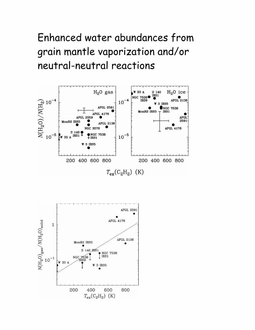
Enhanced water abundances from grain mantle vaporization and/or neutral-neutral reactions

4.13 Kinematics Protostellar outflows easily detected, but how about infall? Evidence from line profile modeling of Evans’ group (V4.10). 4.2 Bipolar outflows and shocks Key motivations for study of shock waves 1) Outflow velocities measured to be supersonic.

(Additional source of shock waves - SN explosions c.f. IC 443)

2) H2 vibrational and high-J CO emissions imply the presence of hot 500 - 2000 K gas in several sources at locations widely removed from an IR continuum source (i.e. a protostar) 4.21 Physics of molecular shocks Shocks compress and heat the gas through which they propagate, converting the kinetic energy of bulk motion into random thermal energy. See review of Draine and McKee 1993, ARAA

Key parameters in shock models: 1) Preshock density 2) Preshock magnetic field ---> 3) Shock velocity 4.211 Fast, dissociative shocks

(see Neufeld 1990 review) Shocks faster than ~ 40 - 50 km/s destroy all molecules that enter them ==> cooling time long: shock front can be viewed as thin adiabatic region within which conversion of bulk k.e. to random thermal energy takes place.

Assume that the “single-fluid” approximation applies: all particles characterized by a common bulk velocity Consider 1-D, steady-state shock wave Jump conditions Equate mass, momentum, and energy fluxes on either side of the shock front. Strong shock limit: preshock gas is highly supersonic, with ρ1v1

2 >> P1, B12/8π

Find that post-shock gas has

ρ2 = 4ρ1 v2 = v1/4 T2 = 3 µv1

2 / 16k ~ 5800 (v1 /10 km/s)2 (for molecular preshock gas)

For v1 > 50 km/s, T2 > 1.5 x 105 K ==> rapid collisional dissociation of molecules

• Subsequent evolution of shocked gas

is governed by radiative cooling, initially by atoms and atomic ions.

• Once temperature drops below 1000

K, molecule reformation takes place. Release of chemical energy associated with H2 formation --> temperature plateau around 500 K (V4.11, 4.12)

4.212 Slow, non-dissociative shocks If molecules survive, the picture can be very different. Molecular cooling is efficient and the ionization is fairly low ==> cooling length << ion-neutral coupling length. Implications: • Ions and neutrals must be treated as

two separate fluids, interpenetrating but weakly coupled. Only the ions are directly coupled to the magnetic field.

• Disturbance can be subAlfvenic with

respect to the ionized fluid: preshock medium “forewarned” and shock discontinuity avoided ==> ‘C’- versus ‘J’-type shocks (Draine 1980).

• `C*’-shocks very similar to ‘C’-shocks

except that there is a sonic point which complicates the computation.

• Peak post-shock temperature can be

considerably smaller than 3µv12 / 16k

Example calculations from Kaufman and Neufeld (1996) (V4.13, V4.14)

4.213 The Wardle Instability To date, nearly all shock modeling involves 1-D simulations. However, Wardle 1990 pointed out that in 2-D or 3-D an instability results in the deformation of the magnetic field (V4.15) Numerical modeling recently carried out by Stone (1997) and by MacLow and Smith (1997) with the ZEUS MHD code. Resultant temperature structure computed by Neufeld and Stone (1997) (V4.16). Can now address the question of whether 1-D, steady-state models are adequate for predicting the emission line spectrum (see 4.3 below). 4.22 Chemistry in molecular shocks

• Elevated temperatures drive neutral-

neutral reactions with large EA • Ion-neutral drift in C-type shocks

preferentially drives ion-neutral reactions with large EA

4.221 J-type shocks Key endothermic reaction is collisional dissociation: H2 + H2 à H2 + H + H - 4.48 eV H2 + H à H + H + H - 4.48 eV

Complete dissociation occurs very rapidly in the very hot region immediately behind the shock front, and the gas is largely ionized. The gas then cools by atomic line emission. Small amounts of H2 (via the H- route) and HeH+ (via radiative association of He+ + H) are expected to form in the warm, ionized gas. Hydrogen molecules reform mainly via grain catalysis gr-H + H à H2 + 4.48 eV and then react with atomic oxygen to form OH

O + H2 < -- > OH + H OH + H2 < -- > H2O + H (back reactions important due to atomic hydrogen, so OH abundance high). OH then reacts further with several species : OH + (S, S+, Si, Si+, N) à (SO, SO+, SiO, SiO+ , NO) + H 4.222 C-type shocks Peak temperatures < 4000 K are not sufficient to significantly dissociate the gas. The composition is nevertheless significantly modified.

Diffuse clouds: Endothermic ion-neutral reactions driven preferentially: Production of CH+ via

C+ + H2 --> CH+ + H - 0.4 eV may explain the “CH+ problem”. SH+ produced by the analogous sulphur reaction, but higher endothermicity makes this effective only at higher shock velocities (and searches for SH+ have always failed)

Dense clouds: Copious water production via

O + H2 --> OH + H OH + H2 --> H2O + H

For shock velocities < 15 km/s (c.f. Kaufman and Neufeld 1996, V4.14), water becomes the dominant reservoir of O not in CO and the dominant coolant of the gas.

4.23 Emission from dense molecular shocks 4.231 Infrared/far-IR line emission Observations: Bipolar outflows often emit:

1) H2 vibrational lines 2) H2 pure rotational lines 3) High-J CO lines 4) H2O rotational lines

Line ratios imply the presence of 500-2000 K gas. OI and SiII fine structure lines are also seen, e.g. towards Orion-KL

J-type shocks Fast, dissociative shocks are fairly weak sources of molecular line emission: most of the cooling occurs before molecules reform. They are luminous sources of OI and SiII fine structure emission, such those observed in the Orion-KL region. C-type shocks Molecules never destroyed, so most of the emission emerges in molecular lines, especially H2 vibrational emissions and H2O rotational emissions.

Models invoking ~ 40 km/s C-type shocks can explain the H2 and CO line strengths observed in Orion-KL (model predictions of Kaufman and Neufeld 1996, V4.17) They can also account successfully for recent ISO observations of

1) water rotational line emission from Orion-KL

2) a non-equilibrium ortho-to-para

H2 ratio in HH54

(indicating that the gas was previously cooler than it is now)

4.232 Water maser emission Although the far-infrared water transitions that dominate the cooling of C-type shocks are observable only from space, several longer-wavelength rotational transitions of H2

16O can be observed from the ground. The first of these was detected thirty years ago by the Townes group:

the 616 - 523 transition at 22 GHz It was quickly realized that this transition exhibited remarkable properties.

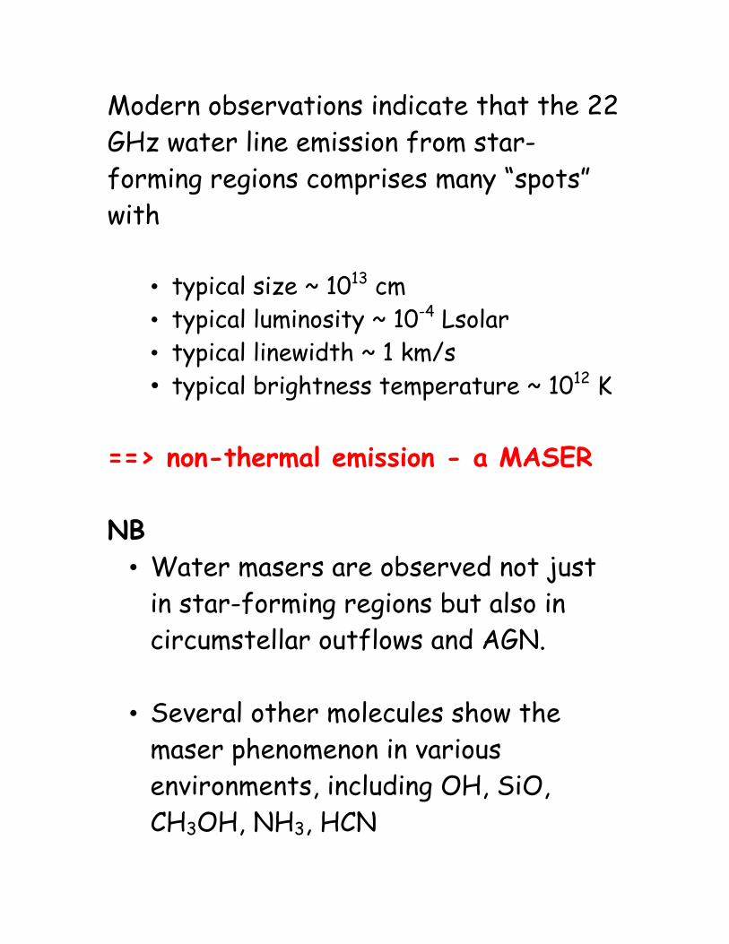
Modern observations indicate that the 22 GHz water line emission from star-forming regions comprises many “spots” with

• typical size ~ 1013 cm • typical luminosity ~ 10-4 Lsolar • typical linewidth ~ 1 km/s • typical brightness temperature ~ 1012 K

==> non-thermal emission - a MASER NB

• Water masers are observed not just in star-forming regions but also in circumstellar outflows and AGN.

• Several other molecules show the maser phenomenon in various environments, including OH, SiO, CH3OH, NH3, HCN

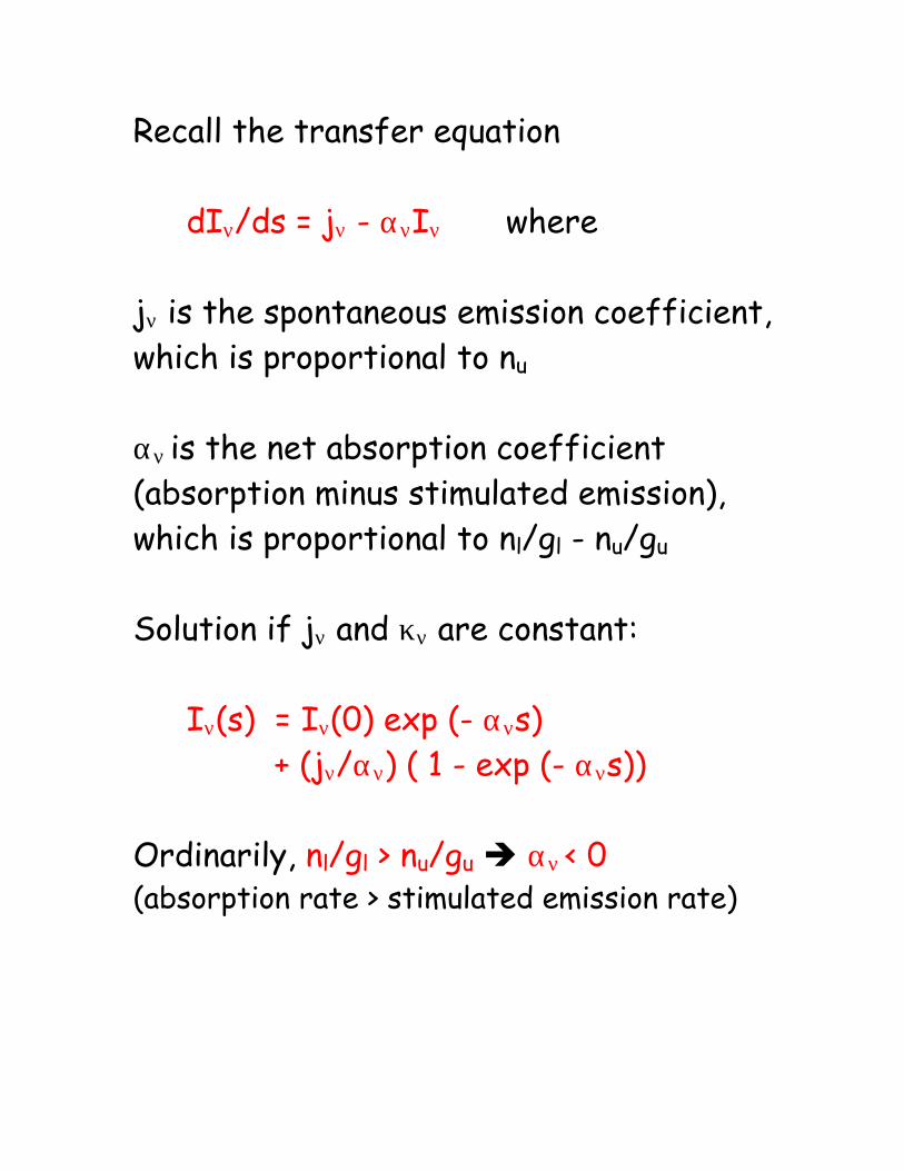
Recall the transfer equation

dIν/ds = jν - ανIν where jν is the spontaneous emission coefficient, which is proportional to nu αν is the net absorption coefficient (absorption minus stimulated emission), which is proportional to nl/gl - nu/gu Solution if jν and κν are constant:

Iν(s) = Iν(0) exp (- ανs) + (jν/αν) ( 1 - exp (- ανs))

Ordinarily, nl/gl > nu/gu è αν

< 0 (absorption rate > stimulated emission rate)

But in unusual circumstances, nu/gu > nl/gl (population inversion) è αν

< 0 (absorption rate > stimulated emission rate) => exp (- ανs) terms grow exponentially Key question: how does the population inversion arise? Amazing result: even though careful arrangements must be made to “pump” the population inversion in laboratory masers and lasers, population inversions arise quite naturally in warm (T > 400 K) interstellar gas (V3.25, V3.26)

Origin of water maser emission in star-forming regions A shock origin is suggested by

1) the temperatures > 400 K needed to form water and excite the masing transitions 2) maser spot proper motions of several x 10 km/s away from the outflow source

Elitzur, Hollenbach and McKee (1989) suggested that the “plateau” region behind a dissociative J-type shock could produce the conditions necessary for water masers.

However, observations of high-lying maser transitions require temperatures hotter than those attained in the plateau region. Kaufman and Neufeld (1996) showed that C-type shocks could account for the relative strengths of the various maser transitions. 4.233 Other radio observations There is also a wealth of radio data on emission from other molecules. Outflow regions typically show enhanced abundances of SiO, H2CO, CH3OH, HCN, SO … and a reduced abundance of HCO+

4.3 OB stars and photodissociation regions Dense molecular clouds are always irradiated by UV radiation, either from the ISRF or a nearby O or B star. Values of IUV as large as 105 have been inferred, leading to “Photodissociation Regions” or “Photon Dominated Regions” (PDRs). Schematic model shown in V4.27 from the review article of Hollenbach and Tielens 1997,ARAA, 35, 179

4.31 Temperature structure Temperature structure determined by the balance between heating and cooling. Heating (V4.28) 1) Photoelectric heating by grains/PAHs Grain + hν --> Grain+ + e + k.e.

with k.e. = hν - φ Grain+ + e --> Grain 2) FUV pumping of H2 H2(X,v=0) + hν --> H2(B,C) H2(B,C) --> H2(X,v=v’) + hν’

with ν’ < ν H2(X,v=v’) + H --> H2(X,v=0) +H + k.e.

Cooling Mainly by atomic fine structure emission:

[CII] 158 micron [OI] 146 micron [SiII] 35 micron [CI] 609, 370 micron

and by H2 and CO rotational lines. At high density, gas-grain cooling can be important Model calculations for the resultant temperature profile from Hollenbach and Tielens shown in V4.29

4.32 Chemistry

Detailed discussion in Sternberg and Dalgarno (1995) (much of which has already been considered in Section 2 above). Two features unique to high-radiation environments are:

• In outer regions, temperatures sufficient to drive reactions of significant endothermicity (e.g. C+ + H2).

• Reactions with vibrationally-

excited H2 also important

e.g. O + H2* à OH + H C+ + H2* à CH+ + H

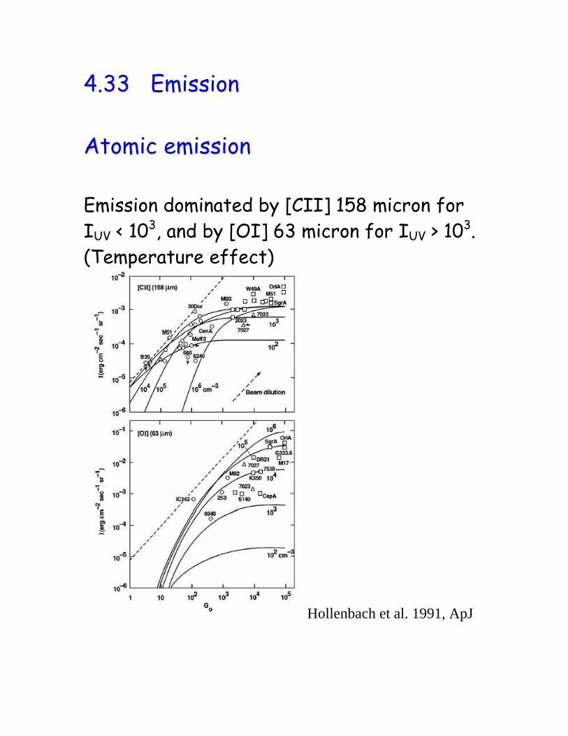
4.33 Emission Atomic emission Emission dominated by [CII] 158 micron for IUV < 103, and by [OI] 63 micron for IUV > 103. (Temperature effect)

Hollenbach et al. 1991, ApJ

FIRAS spectrum of the galaxy shows the dominance of CII

Molecular emission Dominated by mid-J CO lines (e.g. J=7-6) and H2 vibrational lines. Black & van Dishoeck 1989, ApJ

How can be discriminate between H2 vibrational emission from shocks and from PDRs? • In low-density PDRs (nH < 105 cm-3),

vibrational line emission is dominated by fluorescence ==> line ratios independent of gas temperature: based on detailed modeling, we expect [v=1-0 S(1)]/[v=2-1S(1)] ~ 2

• In shocks, we expect “thermal line

ratios” with

[v=1-0 S(1)]/[v=2-1S(1)] ~ exp (6000K/T) ~ 10

Observations: Ratio ~ 10 in some localized regions but ~ 2 over large scales

Luhman & Jaffe 1996, ApJ

Caveat: In high-density PDRs (nH > 105 cm-3), collisional excitation becomes important and drives the ratio upward.

(Sternberg & Dalgarno 1989, ApJ)

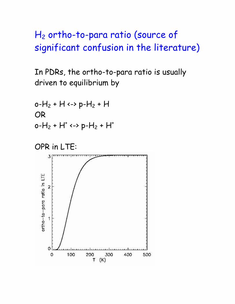
H2 ortho-to-para ratio (source of significant confusion in the literature) In PDRs, the ortho-to-para ratio is usually driven to equilibrium by o-H2 + H <-> p-H2 + H OR o-H2 + H+ <-> p-H2 + H+ OPR in LTE:

However, the OPR in excited vibrational states does not equal the overall OPR Why? Because ortho-states are pumped less effectively than para-states Recall that the pumping rate in very optically-thick lines is proportional to dW/dN(H2) ∝ N(H2)-1/2 Thus, if the true OPR is 3, the vibrational states of ortho-H2 are pumped a factor of √3 less rapidly than those of para-H2.

è column density of vibrationally-excited ortho-H2 is a larger than that of para-H2 by a factor OPR/√3 = 3/√3 = √3 This is confirmed by detailed calculations (Sternberg & Neufeld 1998, ApJ)

5. Circumstellar envelopes 5.1 Astrophysical context All stars lose mass at some level, but mass-loss rates are largest from evolved stars. In particular, Asymptotic Giant Branch (AGB) stars have the largest mass-loss rates (up to 10-4 Msolar yr-1) and are therefore surrounded by the largest, densest, and most molecule-rich envelopes.

Stellar evolution for low-mass stars • Main sequence stars (H burning in core) • Red giants (H burning in shell) • Horizontal branch stars (He burning in core) • AGB stars (He burning in shell)

5.2 Overview Characteristics of AGB stars:

• R ~ 4 x 1013 cm • L ~ 104 Lsolar • Teff ~ 2000 K

Mass loss rate ~ 10-7 - 10-4 Msolar yr-1 Variability on period > 150 days

(pulsational instability)

Circumstellar shell highly optically thick (Av to up to several x 100 mag) Key physics:

• Cool photospheric temperature ==> grain formation at a few stellar radii from surface • Large grain cross-section ==> radiatively-driven wind • Wind reaches terminal velocity at ~

few x 10 stellar radii • Extent of molecular zone limited by

photodissociation by ISRF

Structure:

1) stellar interior 2) stellar photosphere 3) transition zone 4) circumstellar envelope

(Glassgold 1996, ARAA)

5.3 Physical conditions Adopt an idealized, spherically-symmetry and steady-state picture Outflow velocity Dynamics determined by radiation pressure and gravity: Newton’s Law ==> v dv/dR = κ L/(4 π R2c) - GM/R2

The opacity κ can change due to dust formation and to the reddening of the stellar radiation. However, if we adopt a constant κ beyond some dust formation radius Rd, we find that the terminal velocity is given by vt

2 = 2 [(κ L / 4 π c) - G M ]/Rd For L = 104, M = 1 Msolar, Rd = 10 a.u., and κ = 10 cm-1 g-1, we obtain vt = 25 km/s

Comparison of detailed theory and observation (Zubko and Elitzur 2000)

Gas density In steady flow, conservation of mass ==> ρ = dM/dt / (4 π r2 v) ==> nH = 2 x 105 cm-3 (dM/dt)-5 / r16

2 v6 Temperature

Heating processes: gas-grain drift, radiative heating Cooling processes: adiabatic expansion, radiative cooling (by CO or H2O) Result dlnT/dln R ~ - 0.5

Detailed calculation (Zubko & Elitzur 2000)

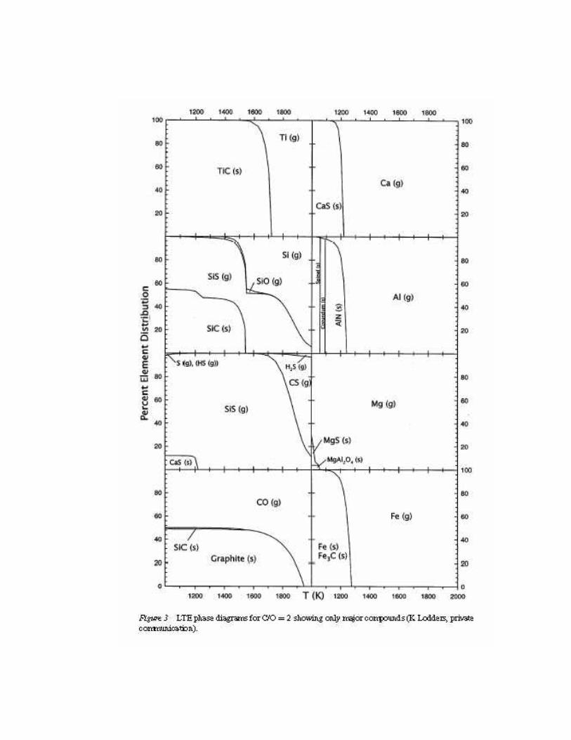
5.4 Circumstellar chemistry Key features 1) Stellar photosphere: thermochemical equilibrium

Chemical state completely determined by thermodynamics for given conditions of ρ and T

2) Outer regions: photodissociation by interstellar radiation field (ISRF)

ISRF important outside radius ~ few x 1016 cm M-5/v6

3) Time dependence important but well defined Flow time = R/v = 317 R16/v6 years

4) Gas phase carbon abundance can be < or > than that of oxygen

Depends on evolutionary phase of star

Carbon-rich envelopes Prototypical example: IRC+10216, a highly-reddened AGB star at a distance of ~ 170 pc. The envelope shows a rich collection of molecular species (Glassgold 1996, ARAA)

Inner envelope: abundances reflect “frozen in” relic of thermochemical equilibrium. Three species dominate:

CO Contains almost all of the O (to be discussed in greater detail soon!)

HCN Contains most of the N C2H2 Contains most of the

remaining C

Outer envelope: photodissociation creates the radicals CN and C2H

HCN + hν --> CN + H C2H2 + hν --> C2H + H

Neutral-neutral reactions involving radicals produce larger species: e.g. C2H2 + CN --> HC3N + H

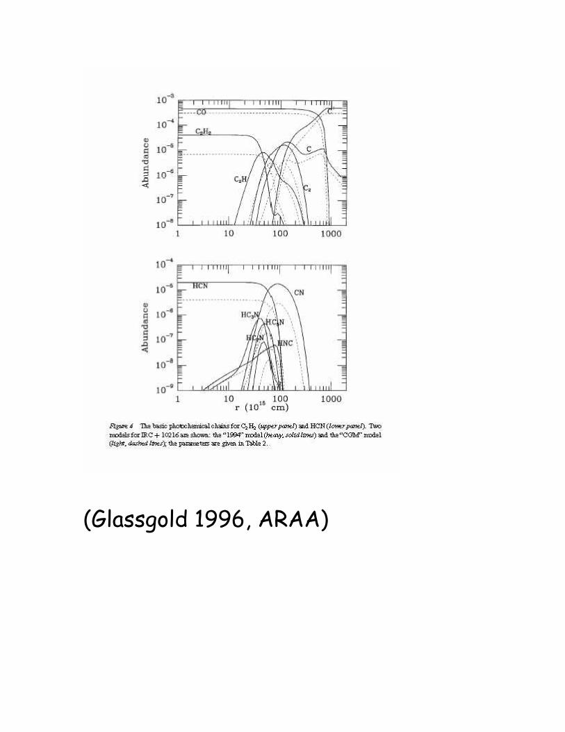
(Glassgold 1996, ARAA)

Oxygen-rich envelopes Prototypical examples:

VY CMa at 1300 pc W Hya at 100 pc Inner envelope: thermochemical equilibrium implies

CO Contains almost all of the C H2O Contains most of the

remaining O

Outer envelope: photodissociation creates a shell of OH

H2O + hν --> OH + H

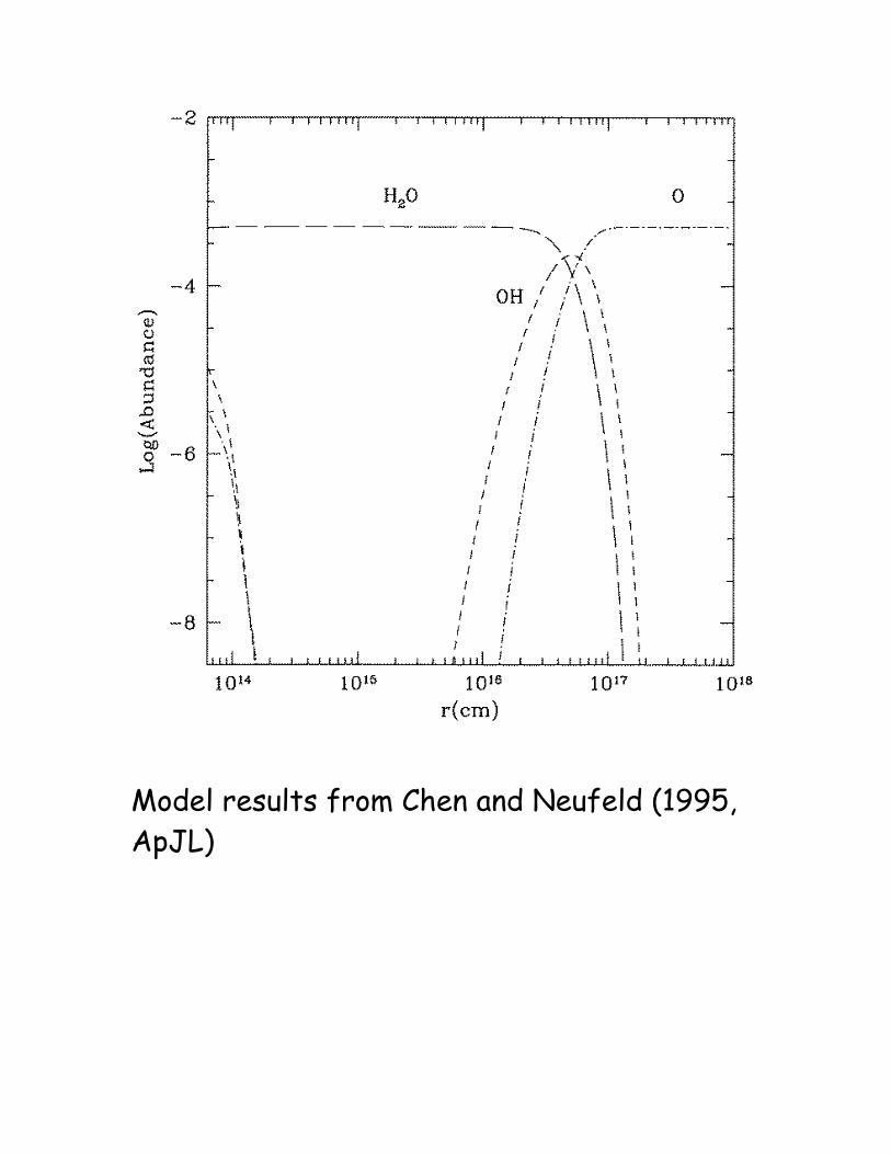
Model results from Chen and Neufeld (1995, ApJL)

5.5 Observations 5.51 Dust continuum observations Dust continuum observations provide a probe of the total amount of ejected material --> dust mass loss rate as a function of time. For constant mass loss rate, intensity inversely proportional to projected distance Example: IRAS observations of W Hydrae (from Hawkins 1990, A&A)

5.52 Radio emission lines Provide information about abundances, given an excitation model. Interferometry --> angular resolution ~ 1 arcsec, equivalent to 3 x 1015 cm for source at 200 pc. Example: molecular rings in observations of IRC+10216 (Guelin and Lucas)

5.53 Maser emission lines In oxygen-rich stars, see shells of maser emission from SiO at R ~ 1014 cm H2O at R ~ 1015 cm OH at R ~ 1016 cm Difference between SiO and H2O maser radii result from differences in critical densities at which the maser transitions are ``quenched’’. Location of OH masers reflects radius at which H2O is photodissociated. Beaming can be radial or tangential.

5.54 Far-infrared emission lines New spectral window opened up by ISO contains the dominant cooling lines for oxygen-rich stars: non-masing rotational transitions of water. First observations carried out toward W Hydrae using the Short Wavelength Spectrometer in Fabry-Perot mode (Neufeld et al. 1996, A&A) Model: observed line fluxes agree with predictions for mass-loss rate ~ few x 10-6 Msolar yr-1

Total luminosity in water lines predicted to be ~ 0.3 Lsolar !! ----> Confirmed by LWS grating scan (Barlow et al. 1996)

6. Comets 6.1 Astrophysical context Small (1 - few x 10 km diameter) mainly icy bodies in orbits beyond ~ 30 a.u. Unprocessed interstellar ices? Small fraction are perturbed onto elliptical orbits that bring them close to the Sun: solar heating à sublimation

Short period comets (P < 200 yr) have prograde orbits with small inclinations to the ecliptic è origin: the Kuiper belt, a flattened belt at 30-100 a.u. from the Sun Recent searches have allowed relatively large objects (D > 50 km) to be detected directly Size distribution: dn/dr ∝ r–4 (1 km < r < 1000 km; Luu and Jewitt 2002, ARAA) Long period comets have an isotropic distribution of orbits è origin: the Oort cloud at ~ 105 a.u. These objects were scattered out of the Uranus/Neptune region early in the history of the solar system

Close to Sun, comets surrounded by a roughly spherical coma (radius ~ 105 km) of gas and dust, and a reflective tail that is driven back by solar radiation pressure. Dirty snowball picture: possible origin of water on Earth. 6.2 Overview Key parameter: Mass outflow rate, typically measured as a water production rate, QH2O, which can be as large as 1031 s-1 The water production rate can be a strong function of heliocentric distance.

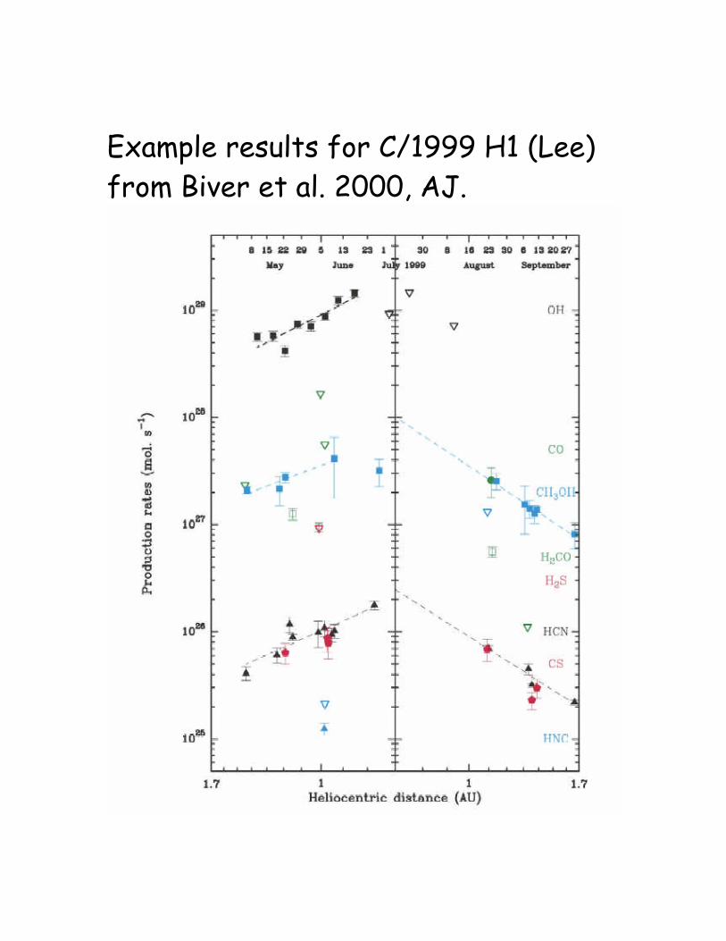
Example results for C/1999 H1 (Lee) from Biver et al. 2000, AJ.

6.21 Physics of cometary comae Key features: • Gas and dust emitted on ballistic

trajectories with at velocity ~ 1 km/s

• Molecular emissions typically

dominated by radiative pumping not collisional excitation, except in the inner coma (D < 100 km)

• Chemistry dominated by

photodissociation with typical destruction timescale ~ 1 day.

• Outer coma is typically optically-thin

to solar UV continuum radiation

6.22 Density profile Density profile of parent molecules typically described by a “Haser” profile, e.g. n(H2O) = (QH2O/4 π r2 v) x exp (-r / [vτH2O]) where τH2O = 1/(photodissociation rate) ~ 105 (R/a.u.)2 sec is the timescale for photodissociation of water by the solar UV field.

Photodissociation timescales depend upon 1) Heliocentric distance (proportional to R2) 2) Solar activity (solar maximum versus minimum) 3) Heliocentric velocity for molecules (such as OH) that are photo-dissociated as a result of line absorption Density distributions for daughter molecules modeled using a “vectorial model” that includes the velocities imparted by photodissociation.

6.3 Cometary molecules 6.31 Atomic and molecular emissions Traditionally (< mid-80s) molecules studied primarily via UV line emissions (IUE and rocket observations). Either:

• pumped directly by solar UV radiation, or

• upper state of daughter

populated following photodissociation of parent

Dominant parent molecule, water, “detected” by means of its photodissociation product OH; CO2 “detected” via CO2

+ and CO. 1986: in situ observations of P/Halley > mid-80’s: observations at radio and infrared wavelengths of transitions that are pumped vibrationally by solar IR radiation; opens up observations of parent molecules. Observations carried out from a variety of telescopes, including KAO, IRTF, ISO, SWAS and ODIN.

Direct observations of water vapor have now been carried out è old method of observing OH works quite well Example: SWAS observations of C/1999 H1 (Lee) – Chiu et al. 2000, Icarus

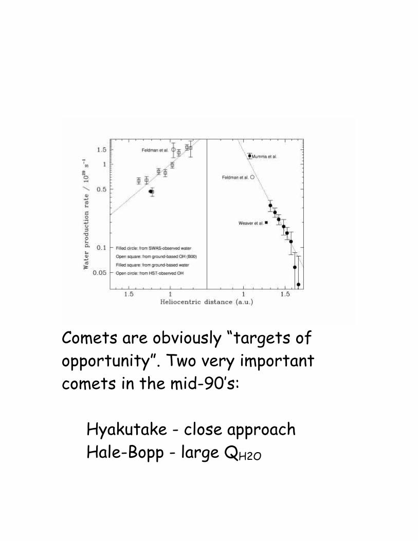
Comets are obviously “targets of opportunity”. Two very important comets in the mid-90’s:

Hyakutake - close approach Hale-Bopp - large QH2O

6.32 Cometary composition Very hard to observe ices directly: so observe molecules in gas phase after they have been vaporized. Summary of results in Bockelee-Morvan table, with production rates normalized w.r.t. water = 100 Important point: production rates determined by sublimation temperatures as well as cometary composition e.g. CO/H2O and CO2/H2O larger when comet is further from Sun

Major components: H2O CO CO2

CH3OH Bottom line: nuclear composition does appear to reflect that of interstellar ices, with coma composition reminiscent of hot core regions. Caveat: There is clearly evidence for some processing – presence of crystalline silicates (narrow 11.2 micron feature) implies annealing at high temperature (T > 1000 K)

Crovisier et al. (1996, A&A)

Other evidence: Water ortho-to-para ratio ~ 2.5 è water ice originally froze out from water in LTE at ~ 30K Detection of HDO implies HDO/H2O ~ 3 x 10-4, very similar to hot core regions (and 2 x Earth’s oceans).

Cometary origin for Earth’s oceans? HDO/H2O ratios measured in Halley, Hale-Bopp and Hyakutake seem to high for Earth’s oceans to have been delivered primarily by comets However, Mumma (2001, Science) has pointed out that a separate class of comets (“Jupiter-family”) has a markedly different composition C/1999 S4 LINEAR: CO, CH4, C2H6, C2H2 are significantly underabundant compared to most short-period comets è suggests a warmer formation temperature that might give less HDO fractionation

6.4 Comets around IRC+10216? Very surprising result from SWAS: detection of water vapor toward IRC+10216 (Melnick et al. 2000) Required VERY long integration – testament to the stability of the SWAS receivers

• Dredge-up” of carbon from the

core has made the entire star “carbon-rich”, with a carbon/oxygen ratio ~ 1.4 to 2

- Chemical models predict almost

all oxygen in form of CO - Predicted water abundance,

H2O/H2, is ~ 10-12, far below the SWAS detection threshold

• Yet the H2O abundance implied by

SWAS observations is ~ 10-6

Favored explanation of water vapor detected in IRC+10216 (Ford & Neufeld 2000, ApJL): a collection of orbiting icy bodies, analogous to the Solar System’s Kuiper Belt, is being vaporized by the large luminosity of the star.

Current stellar luminosity is ~ 104 Lsolar è even objects as large as Pluto will have been vaporized if they lie within ~ 75 AU of the star

Objects at distances ~ 75 – 300 AU (distance of Sedna) are currently being vaporized and are dumping water vapor into the outflow

Vaporization wave spreads outwards as stellar luminosity increases

Required mass of water ice ~ 10 Earth masses, comparable to the initial mass inferred for our KB

Alternative explanations appear to be unsuccessful 1) Shocks in the inner envelope? Might break apart CO, producing O that could react with H2 to form H2O But would also break apart H2, producing H which is not seen (21 cm upper limits) and which would destroy H2O Photodissociation in the outer envelope

2) Ambient Galactic UV field eventually destroys CO But only in outer region where conditions are unfavorable for H2O formation peak water abundance ~ 10-11 according to model of Millar & Herbst Also, water in outer region is excited much less effectively – this outbalances the larger beam filling factor since volume emissivity dL/dV ∝ n2 ∝ r–4 è dL/dlogr ∝ r–1

Summary Water detection toward IRC+10216 argues for the presence of a planetary system around another star SWAS observations demonstrate the potential of molecular spectroscopy as a probe of extra-solar planetary systems

Method is complementary to the now standard method of searching for periodic Doppler shifts in stellar spectra

• Doppler shift method: sensitive only to discrete large bodies (mass ~ MJ) at small distances (< few AU).

• Water observations: sensitive to populations of small icy bodies (comet-sized) at large distances (~ 100 AU) around carbon-rich AGB stars

Ground-based observations

• Detection of OH (Ford et al. 2003) – the expected photodissociation product of water

• Line flux agrees with expectations, but absence of red “horn” is unexpected:

- Asymmetric vaporization? - Maser amplification?

• Detection of H2CO (Ford et al. 2004) – another cometary volatile that is not expected in a C-rich environment

Derived H2CO/ H2O ratio ~ 4% is comparable to the value typically measured in solar system comets As in comets, H2CO appears to be a daughter (photodissociation) product Key tests of the comet vaporization hypothesis

1) Detection of deuterated species would clinch the cometary origin (HDO, HDCO) 2) Line strengths of far-IR transitions (Herschel Space Observatory)

Significance of Herschel • Herschel/HIFI is ~ 1000 times more

sensitive than SWAS to emission from unresolved sources è significant expansion of discovery space: ~ 10 candidate C-stars will be targeted

• HIFI can detect far-IR water lines: line

ratios probe the spatial distribution of the water and provide a test of the comet vaporization hypothesis (preliminary results below from Ford et al. 2001)

Transition Wavelength

(mm) Flux (W cm-2) Rw= 0

Flux (W cm-2) Rw=100 AU

F/F(110-101) Rw= 0

F/F(110-101) Rw =100 AU

110-101 * 538.27 1.404 (-20) 1.137 (-20) 1.000 1.000 212-101 179.53 1.311 (-19) 6.420 (-20) 9.335 5.647 221-212 180.49 4.049 (-20) 1.012 (-20) 2.884 0.8900 303-212 174.62 9.508 (-20) 2.463 (-20) 6.772 2.166 312-221 259.99 1.839 (-20) 1.636 (-21) 1.310 0.1439 312-303 273.20 1.031 (-20) 1.726 (-21) 0.7346 0.1518 321-312 257.79 7.092 (-21) 5.808 (-22) 0.5052 0.05109 523-514 212.52 6.262 (-21) 4.111 (-24) 0.4461 3.616 (-4) 532-523 160.51 1.604 (-20) 1.217 (-24) 1.143 1.071 (-4) 734-725 166.81 7.727 (-21) 9.008 (-27) 0.5504 7.923 (-7)

7. Accretion disks Reference: Accretion power in astrophysics by Frank, King and Raine (Cambridge 1985, 1992) 7.1 Astrophysical context The accretion process is central to astrophysics. For accretion onto an object of mass, M, and radius, R, an accretion disk forms if the the accreting material has specific angular momentum > (GMR)1/2.

Examples:

• Binary stars, especially X-ray binaries (atomic)

• Protostars

(molecular)

• Active Galactic Nuclei (AGN) (molecular)

For protostar case, see Cassen & Moosman infall solution (V7.1) with rd ~ 100 a.u.

7.2 Physics of thin accretion disks In many astrophysical systems, we expect an accretion disk that is thin and nearly-Keplerian; this is the case we will consider here. Thin ç turbulent + thermal motions << orbital velocity Nearly-Keplerian ç disk mass << central mass

7.21 The Physics of Accretion Keplerian motion è differential rotation, with dΩ/dR < 0 Without dissipation, material would remain in circular motion at fixed radius: vφ = (GM/R)1/2

= 30 km/s (M/Msolar)1/2 Ra.u.-1/2

vr = 0 But, due to viscosity, outer parts of disk exert retarding torque on inner parts.

Definition of viscosity: Torque per unit area = ν ρ dvy/dx (in plane-parallel symmetry) Consequences:

• Frictional energy dissipation heats disk

• Angular momentum transported outwards

• Material transported inwards in tight spiral (vr < 0)

Key unknown: origin and magnitude of viscosity (involves magnetism?)

Shakura-Sunyaev parameterization: ν = α cs H where H is the disk thickness and α is a dimensionless number (~ 1 ??) In steady-state solution to disk, it can be shown from considerations of mass and momentum conservation that: vr = 3ν/2R far from the inner boundary è mass accretion rate

= 2πRvrΣ = 3πνΣ = 3παcsΣH

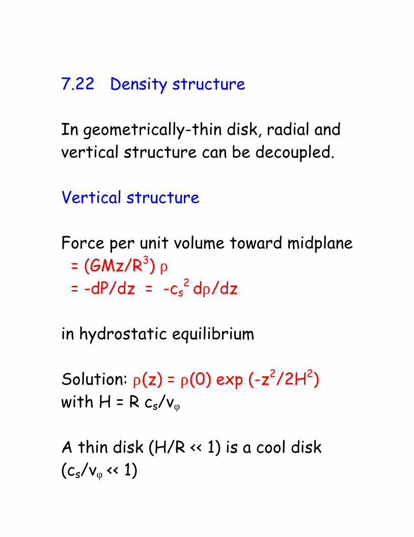
7.22 Density structure In geometrically-thin disk, radial and vertical structure can be decoupled. Vertical structure Force per unit volume toward midplane = (GMz/R3) ρ = -dP/dz = -cs

2 dρ/dz in hydrostatic equilibrium Solution: ρ(z) = ρ(0) exp (-z2/2H2) with H = R cs/vφ A thin disk (H/R << 1) is a cool disk (cs/vφ << 1)

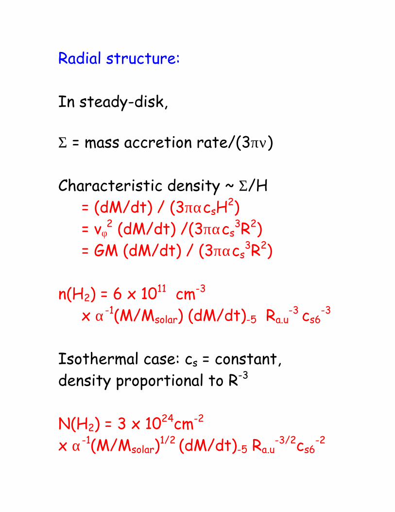
Radial structure: In steady-disk, Σ = mass accretion rate/(3πν) Characteristic density ~ Σ/H

= (dM/dt) / (3παcsH2) = vφ

2 (dM/dt) /(3παcs3R2)

= GM (dM/dt) / (3παcs3R2)

n(H2) = 6 x 1011 cm-3

x α-1(M/Msolar) (dM/dt)-5 Ra.u-3 cs6

-3

Isothermal case: cs = constant, density proportional to R-3 N(H2) = 3 x 1024cm-2 x α-1(M/Msolar)1/2 (dM/dt)-5 Ra.u

-3/2cs6-2

7.23 Disk heating Conservation of energy ==> viscous dissipation rate per unit area, D(R) = GM(dM/dt)/(4πR3) (average over disk) Disk may also be heated by external irradiation (optical, X-ray)

7.3 Molecules in protostellar accretion disks Disk temperature is conducive to existence of molecules In protostellar accretion disks, illumination by the central protostar dominates the heating. Disk is highly-optically thick, so σT4 = F Note that F decreases as R-3 not R-2, because of obliquity factor (so heating rate coincidentally shows same dependence as viscous heating). T ~ few x 100 K (R/a.u.)3/4 Over a wide range of radii, gas is warm, dense and molecular.

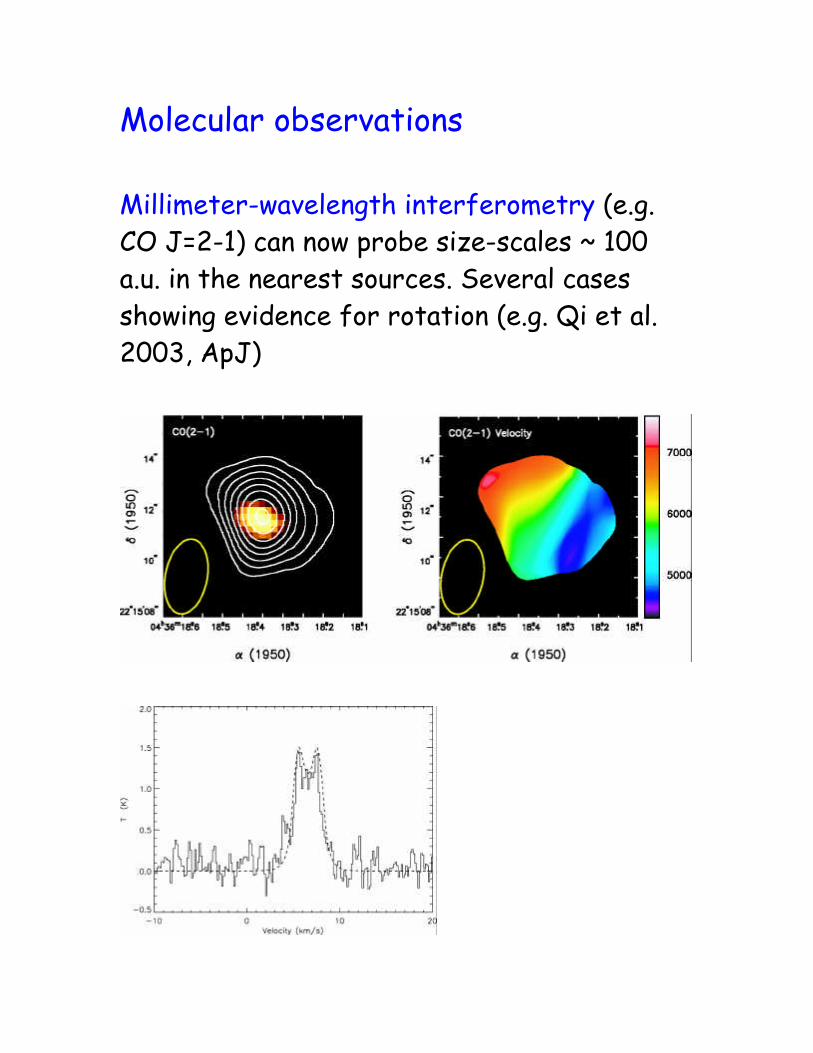
Molecular observations Millimeter-wavelength interferometry (e.g. CO J=2-1) can now probe size-scales ~ 100 a.u. in the nearest sources. Several cases showing evidence for rotation (e.g. Qi et al. 2003, ApJ)

Alternative method: use spectral line profiles to probe rapidly-rotating inner regions. CO vibrational transitions widely observed from protostars - likely disk origin. From ground, easiest to observe CO v = 2-0. High critical density and high excitation energy (E/k ~ 6000 K) make this transition a good tracer of the warm, dense inner disk.

Band profile represents convolution of vibrational band shape with kinematic profile for Keplerian disk of inner radius, Rin

Good fit to WL 16 and 1548C27 (Najita et al. 1996).

(WL16 example) Caveats: 1. Emission lines è temperature inversion in disk (dT/dz < 0) (like chromospheric lines in stars) External irradiation does not appear to produce a sufficient temperature inversion. Other possibilities: disk-wind interaction, heating by MHD waves

2. Other possible sources of CO vibrational lines: a) Accretion shocks (Neufeld and Hollenbach 1994):

• Yield narrower lines (as indeed

observed in some sources e.g. SVS 13)

• Can only match CO v=2-0 luminosities of some sources

• Possible explanation of cm

wavelength Bremsstrahlung (Neufeld and Hollenbach 1996, ApJL)

b) Stellar winds (Ruden, Glassgold & Shu 1990)

• Only bright enough if mass

outflow rate large • Expect asymmetric line profiles

due to occulation of receding lobe and absorption of stellar radiation by approaching lobe

Administrator

8. Molecules in the Early Universe Here we consider possible effects of molecules at z = 10 - 1000 prior to the first generation of stars. 8.1 Motivation Prospects for observing molecules at this epoch are dim. However, even small amounts of molecules can be important for cooling.

1) Molecules are potentially important coolants because they alone have low-lying energy states in gas of primordial composition. Baryonic content of Early Universe: H: D: He: Li ~ 1: 10-4: 0.1: 10-10 None of these atoms (or their ions) have low-lying transitions => atomic cooling always dominated by H Lyα which is ineffective below ~ 10,000 K (since ∆E/k ~ 158,000 K) However, H2 has a lowest excitable state (J = 2) at ∆E/k ~ 500 K (and HD and LiH have lower states still).

2) Temperature is critical in regulating gravitational collapse Collapse is resisted by thermal pressure. Jeans criterion: Jeans wavelength:

λJ = (π γ k T / m G ρ)1/2 ==> Jeans Mass = (π λJ

3/6) ~ 56 (T/K)3/2

(n/cm-3)-1/2 solar masses

Jeans mass is 1000 times smaller if T=100 K instead of 10000 K

Note that for adiabatic collapse in γ = 5/3 gas, T increases as n-2/3 è MJ increases at n-1/2 è collapse stabilized Collapse is impossible without cooling.

8.2 Formation of molecules in gas of primordial composition 8.21 Molecular hydrogen No grains! è normal grain-catalysed H2 formation is impossible However, H2 can be produced in the gas-phase via two routes: 1) Formation via H- H + e --> H- + hν

(radiative attachment) H- + H --> H2 + e

(associative detachment)

At z > 200, this route is strongly inhibited by photodetachment (only requires hν > 0.75 eV): H- + hν --> H + e 2) Formation via H2

+ H + H+ --> H2

+ + e (radiative association)

H2+ + H --> H2 + H+ (charge transfer)

Destruction Radiation field: pure blackbody at T = 2.73(1+z) K (at least until first generation of stars forms) ==> no UV capable of photodissociating H2 Result: Molecular hydrogen abundance reaches few x 10-6 by z = 100 (c.f. Lepp and Shull 1984; Latter 1989)

Once stars form, several new effects (e.g. Haiman et al. 1997)

1) Heavy element and dust formation

2) Ionization increases gas-phase H2 formation rate

3) Photodissociation by stellar UV

8.23 Other molecules HD HD forms via reactions entirely analogous to those that form H2

(Radiative association also possible but negligible.) HD abundance reaches ~ 10-9

LiH LiH can form via Li- route (analogous to H- route) or via radiative association of Li and H. LiH abundance reaches ~ 10-16 (Stancil et al. 1996)

8.3 Cooling and temperature evolution Even though HD and LiH have 1) lower energy states 2) higher critical densities H2 cooling usually dominates due to its much larger abundance. Old Lepp and Shull (1984) results show evolution of cloud that starts collapsing at z=50

Without any cooling, T would increase as n2/3

Without molecular cooling, H Lyα would stabilize the temperature around 10,000 K. With molecules, temperature limited to several hundred K.

è Jeans mass reduced by factor ~ 100