1 introduction - universit degli studi di padova

0

UNIVERSITÀ DEGLI STUDI DI PADOVA

Dipartimento di Ingegneria Industriale

Tesi di laurea

ESTIMATION OF ECONOMICAL AND ENVIRONMENTAL BENEFITS FROM

DEPLOYMENT OF MICRO CHP TECHNOLOGIES IN A DETACHED HOUSE IN

ITALIAN CLIMATIC CONDITIONS

RELATORE: PROF. MICHELE DE CARLI CORRELATORE: PROF KHAMID MAHKAMOV

LAUREANDO: GIACOMO TAVERNARO

Anno Accademico 2012/2013

1

CONTENTS

1 INTRODUCTION....................................................................................................................7

1.1 RESEARCH BACKGROUND..................................................................................................7

1.2 PROJECT DESCRIPTION......................................................................................................8

2 LITERATURE REVIEW............................................................................................................9

3 TIPE OF MCHP TECHNOLOGIES..........................................................................................18

4 COMMERCIALY AVAILABLE SYSTEMS................................................................................20

4.1 RECIPROCATING INTERNAL COMBUSTION ENGINE........................................................20

4.2 MICRO GAS TURBINE.......................................................................................................23

4.3 MICRO RANKINE CYCLE (MRC) ........................................................................................25

4.4 STIRLING ENGINE.............................................................................................................28

5 CURRENT STATES OF INVESTIGATIONS.............................................................................33

5.1 SISTEMA TERMOFOTOVOLTAICO TPV.............................................................................33

5.2 CELLE A COMBUSTIBILE FC..............................................................................................36

6 THEORETICAL BACKGROUND OF MODELLING SOFTWARE...............................................40

7 DWELLING DESCRIPTION...................................................................................................43

7.1 DOMESTIC AND OCCUPANCY CHARACTERISTICS............................................................43

8 MODELLING OF THE HOUSE WITH A BOILER.....................................................................49

9 MODELLING OF THE HOUSE WITH A ICE...........................................................................53

9.1 INTERNAL COMBUSTION ENGINE PLUS AUXILIARY BOILER WITH GAS FIRED BOILER FOR

DHW......................................................................................................................................53

9.2 INTERNAL COMBUSTION ENGINE PLUS AUXILIARY BOILER SPLIT GENERATION

STRATEGY..............................................................................................................................56

9.3 NETWORK INTERACTION.................................................................................................59

10 MODELLING OF THE HOUSE WITH A STIRLING ENGINE..................................................64

10.1 STIRLING ENGINE PLUS AUXILIARY BOILER WITH GAS FIRED BOILER FOR DHW...........64

10.2 STIRLING ENGINE PLUS AUXILIARY BOILER SPLIT GENERATION STRATEGY..................68

2

10.3 NETWORK INTERACTION...............................................................................................70

11 ANNUAL SUMMARY.........................................................................................................75

11.1 ECONOMIC PERFORMANCE...........................................................................................75

11.1.1 Analysis without parasitic electric load and all taxes excluded price........................76

11.1.2 Savings with parasitic electric load and all taxes excluded price...............................78

11.1.3 Analysis without parasitic electric load and all taxes included price.........................78

11.1.4 Savings with parasitic electric load and all taxes included price...............................80

11.2. CARBON SAVINGS.........................................................................................................80

12 CONCLUSIONS..................................................................................................................82

13 REFERENCE.......................................................................................................................84

APPENDIX I............................................................................................................................88

APPENDIX II...........................................................................................................................89

APPENDIX III..........................................................................................................................90

APPENDIX IV.........................................................................................................................91

3

FIGURES

Figure 3.1: Energy flows of alternative (MCHP) and conventional (power plant and boiler)

systems..................................................................................................................................18

Figure 7.1.1: design of single house......................................................................................43

Figure 7.1.2: electrical load distribution in a typical weekday..............................................46

Figure 7.1.3: electrical load distribution in a typical weekend day.......................................47

Figure 7.1.4: temperature zones profile with no heating systems........................................48

Figure 8.1: weekday electrical demand, boiler gas consumption, water heater gas

consumption, cookers gas consumption profile...................................................................49

Figure 8.2: weekend day electrical demand, boiler gas consumption, water heater gas

consumption, cookers gas consumption profile...................................................................50

Figure 8.3: DHW during weekday..........................................................................................51

Figure 8.4: DHW during weekend day...................................................................................51

Figure 8.5: boiler operation and temperature zones profiles during a winter weekday......52

Figure 9.1.1: fuel consumption and thermal energy produced for mCHP and boiler for a

winter weekday.....................................................................................................................54


warm weekday......................................................................................................................54

Figure 9.1.3: boiler and mCHP operation and temperature zones profiles during a winter

weekday................................................................................................................................55

Figure 9.1.4: mCHP operation and temperature zones profiles during a winter weekday

without boiler........................................................................................................................56

Figure 9.2.1: operation characteristics of the mCHP and boiler and the dhw profile in a

winter weekday.....................................................................................................................57

Figure 9.2.2: temperature inside the tank and consumption of hot water in a winter

weekday................................................................................................................................57

Figure 9.2.3: operation of mCHP and dhw heating demand during a weekday....................58

Figure 9.2.4: operation of mCHP and dhw heating demand during a weekend day.............58

Figure 9.3.1: electricity produced by mCHP unit, surplus, energy purchased and electric

demand in a winter weekday................................................................................................59

Figure 9.3.2: electricity produced by mCHP unit, surplus, energy purchased and electric

demand in a winter weekend day.........................................................................................60

4

Figure 9.3.3: electricity produced by the mCHP unit under split pattern, surplus, energy

purchased and electric demand in a winter weekday...........................................................61


purchased and electric demand in a winter weekend day....................................................61

Figure 9.3.5: annual export proportion for mCHP plus boiler for DHW................................62

Figure 9.3.6: annual export proportion for mCHP with split generation strategy.................62


winter weekday.....................................................................................................................65


warm weekday......................................................................................................................66


weekday................................................................................................................................67


without boiler........................................................................................................................67


winter weekday.....................................................................................................................68


weekday................................................................................................................................69

Figure 10.2.3: operation of mCHP and dhw heating demand during a weekday..................69

Figure 10.2.4: operation of mCHP and dhw heating demand during weekend day.............70

Figure 10.3.1: electricity produced by the mCHP unit, surplus, energy purchased and,

electric demand in a winter weekday...................................................................................71

Figure 10.3.2: electricity produced by the mCHP unit, surplus, energy purchased and

electric demand in a winter weekend day............................................................................71


purchased and electric demand in a winter weekday...........................................................72


purchased and electric demand in a winter weekend day....................................................73

Figure 10.3.5: annual export proportion for mCHP plus boiler for DHW..............................73

Figure 10.3.6: annual export proportion for mCHP with split generation strategy:.............74

5

TABLES

Table 3.1: characteristics of mCHP systems..........................................................................19

Table 4.1.1: Testing of the Micro-CHP ‘‘Dachs”.....................................................................22

Table 4.1.2: Testing of the Micro-CHP ecopower..................................................................22

Table 4.2.1: features of micro gas turbine............................................................................25

Table 4.3.1: features micro Rankine units.............................................................................28

Table 4.4.1: Testing of the Micro-CHP SOLO Stirling 161. ....................................................31

Table 4.4.2: Testing of the Micro-CHP SM5A........................................................................32

Table 5.1.1: TPV costs............................................................................................................35

Table 5.2.1: principal features of fuel cells............................................................................37

Table 5.2.2: mian available prototypes.................................................................................38

Table 7.1.1 Table 7.1.7: construction details............................................................4447

Table 11.1.1.1: annual economic performance for all scenarios with feed-in-tariff of 50 % of

the purchase price.................................................................................................................76



Table 11.1.1.3: annual economic performance for all scenarios with feed-in-tariff of 100 %

of the purchase price.............................................................................................................77

Table 11.1.2.1: annual economic savings for all scenarios taking into account the parasitic

electric load...........................................................................................................................78





Table 11.1.3.3: annual economic performance for all scenarios with feed-in-tariff of 100 %

of the purchase price.............................................................................................................79

Table 11.1.4.1: annual economic savings for all scenarios taking into account the parasitic

electric load...........................................................................................................................80

Table 11.2.1: annual carbon emissions predicted for all scenarios without parasitic electric

load........................................................................................................................................81

6

Table 11.2.2: annual carbon savings predicted for all scenarios with parasitic electric

load........................................................................................................................................81

NOMENCLATURE

°C Temperature in Celsius

kWh Energy in kilo Watts

kW Power in kilo Watts hours

e Electric

th Thermal

L Volume in litres

y Year

m Metres

7

1 INTRODUCTION

CHP is the acronym of cogeneration heat and power. It means the instantaneously

production of heat and electrical power. Indeed CHP systems are developed to produce

electric power with the advantage of supplying thermal energy for heating and cooling [1].

The first and more interesting advantage is the high efficiency which can achieve around

85-90 % [2]. Lately the micro CHP technologies, applied to the domestic uses, arouse

interest. There is no agreed size limit but 10 kW of electrical power may be appropriate for

domestic sector [3]. Some papers report that in the smallest size, fuel cells and Stirling

engines are viewed as the most applicable technologies. The future market developments

will be different depending on the countries. Three countries, Germany, UK and The

Netherlands, will become the largest market installations; this is favoured by the climate,

and a developed gas connection rate. A second group of countries, composed of Italy,

Switzerland, Austria and Belgium, will play an important role in the mCHP diffusion. The

rest of the Europe, are not interested in this solution due to the lack of gas connection and

the moderate climate [4].

1.1 RESEARCH BACKGROUND

The mCHP is become an important part of the daily day, both for the social and the

economic aspect. In fact in the last 20 years the attention has been focused to find new

energy systems, trying to combine the request of environment friendly technology and

customer demand.

In particular the new technologies and energy engineer studied are developed in order to

find a successful combination between low energy consumption and low energy

dispersion.

These aspects have started to have a big impact not just in industrial field, but also in the

economic and social one, since the petrol crisis has started in the 90’s.

The source of new energy device has been pushed further in the last 10 years, by the

industry and the European governments as well. In particular the attention is focused to

find a way to decrease the consumption of primary energy and to decrease the carbon

emissions by using opportune structure and CHP system.

8

Since the beginning of the 2000 various studies about the factors affecting the operational

environment and obstacles limiting the market of small-scale have been done. Thus have

permitted to amply the study of this field and finally to find the way to improving the

situation. Many studies have tried to compare different mCHP prime mover, in order to

find the best solution taking into account economic and environmental benefits. The

climatic conditions and dwelling characteristics affected the results.

The importance of the discovery and the development of new energy system have an

important impact in everyday life, in economics and in politics.

1.2 PROJECT DESCRIPTION

A detached house in Italian climatic condition had been modelled using a free software

called Energy Plus. Three different prime mover had been taken into account to cover the

thermal demand for the space heating and hot domestic water: a conventional boiler, an

internal combustion engine and a Stirling engine. Annual and daily simulations were carried

out and the results were compared. At the end economical and environmental benefits

were determined for each system.

9

2 LITERATURE REVIEW

Nelson Fumo et al. [1] (2009) presented a mathematical analysis. They demonstrated that

CHP systems increased the energy consumption on-site. After a little description of

different CHP systems it was demonstrated the increasing for three different operation

modes: the first was cooling, heating, and power; the second was heating and power; and

the last was cooling and power. In the first operation the building–CHP system increased

the site energy consumption, also in the second, where the operation was made for

recovered thermal energy equal recovered and available thermal energy for heating

(Qr=Qra), but usually Qr>Qra, so the site energy consumption increased. Kari Alanne and

Arto Saari [2] (2004) showed factors affecting the operational environment, obstacles

limiting the market of small-scale and they tried to delineate how improving the situation.

At the end there is a little description of different CHP systems and a confront of these

devices. They affirmed that for a detached house is better to install Stirling engines or fuel

cells, and not reciprocating engines or gas micro-turbines. Mark Hinnells [3] (2008) spoke

about the UK situation. In UK the situation regarding the mCHP market was not just

affected by a lack of improve of technological changes, but by political factors. Indeed the

policy plays an important role as CHP typically could save around 500000-760000 tonnes of

carbon per 1000 MWe installed capacity. In the paper the mCHP technology was called

Cinderella technology in term of sustainable energy policy and it means that the UK

Government has not supported this type of thecnology. M. Dentice d’ Accadia et al. [4]

(2003) presented the state of art of the principal mCHP technologies and the market

prospects for the European countries. They developed two different tests, consisted of two

different sections: the first outdoor unit contained the mCHP module while in the second

all the thermo-electric house system were arranged, permitting the simulation of thermal

and electrical loads. The performance of mCHP system and the optimum operation mode

were evaluated in order to match the user’s thermal and electrical loads. Peter Asmus [5]

(2001) offered a unusual point of view concerning the energy, connected with the

terrorism. The central power plant presented in the paper was affected by some problems

like the losses and a way to fix the problem will be the installation of cleaner and smarter

power sources. It has been shown how the costs of fossil and nuclear generators continue

to add up. Therefore the costs increase while national security decreases. In the author’s

opinion a new smarter and cleaner distributed model, like microgenerators, could mitigate

10

also this problem. R. Possidente, et al. [6] (2006) at the beginning spoke about the

European market restriction which did not allow to the mCHP technologies to be available

in the market. The paper showed an experimental analysis conducted in a several ranges of

operating conditions performed on three different mCHP prototypes. The energetic,

environmental and economic performances were studied and compared with a reference

scenario consisted of a boiler to cover the heating demand. The mCHP systems studied

were three, with a electrical power respectively of 3 kW 1.67 kW and 6 kW. The

comparison with conventional system showed that the first mCHP system allowed a

reduction of gas emission of 20 %. The third device had always a lower emissions than the

conventional system, reaching also 40 % of the avoided emissions. The results savings

demonstrated how it was possible saving up to 25 %, of energy using primary source. M.

Bianchi and P. R. Spina [7] (2010) focused the attention in the small size micro CHP,

excellent systems for residential heating. They studied general operations and

performances of the most important devices for the domestic application in Italy, focusing

the attention in the evaluation of primary energy saving compared to conventional

systems. They also investigated the problems caused by the connection between the micro

CHP systems and the grid and the restrictions to the market availability. M. Bianchi et al.

[8] (2009) also wrote about other mCHP technologies, in particular those characterized by

nominal electrical power under 1 MW. This size has been chosen because it corresponds

to the maximum nominal power by law for the micro CHP systems in Italy (D. Lgs. n.

20/07). In the paper all systems have been investigated and described, paying more

attention to the operation rather than the energetic and environmental performance.

Furthermore little information have been given about the market potentiality and the

principal using. In fact there is lack of a practical analysis of the technologies that showed

relevant features, since few real plants built in Italy have been described. Bernd Thomas [9]

(2008) showed in this paper the test results made on two different types of cogeneration

engines. The devices studied were: two internal reciprocating engines (SenerTec ‘‘Dachs”

and Micro-CHP ecopower by PowerPlus Technologies) and two Stirling engines (SOLO

Stirling 161 Micro-CHP unit and Micro-CHP SM5A by Stirling Denmark). The paper gives an

exhaustive description and comparison between the two systems regarding the

performance, electrical efficiency, thermal efficiency, and the CO and NOx emissions. At the

end the different systems were compared. The commercially available units (SenerTec

11

‘‘Dachs”, SOLO Stirling and ecopower unit) seemed well developed and suitable to cover

the demands of the customers. For economic consideration, the cost was around 3000

€/kWe, too high to allowed beneficial operation for single family users. E. S. Barbieri et al.

[10] (2012) at the beginning of the paper tried to calculate: thermal energy demand,

cooling demand, and the electrical energy demand for a single family. The range of primary

energy for hot water was considerably large and it ranged from 10 to 300 kWh/(m2y),

instead electric energy demand was slightly higher than 25 kWh/(m2y) in Italy. In the

second part the economical point of view was evaluated. It was shown the primary energy

saving and CO2 savings for two different house: the first smaller ( 96 m2) than the second

(200 m2), where several different types of micro CHP systems were installed. It was noted

that the marginal cost per unit of installed electric power was in the range of: 600–1800

€/kWe for the first building and PBP (payback period) = 10 years and 2200–6600 €/kWe for

the second building and PBP = 10 years. C. Roselli, et al. [11] (2011) examined the

performance of different micro CHP systems. It was taken into account internal

reciprocating engines and Stirling engines. Typical heating systems composed of boiler that

cover the thermal demand was compared. In the reference scenario the electricity was

taken by the grid. Also they compared the primary energy saving and CO2 savings. The

primary energy saving was evaluated by the PES index. Those were the values: for boiler

the efficiency is 85.0 %, CO2 equivalent emission = 0.20 kgCO2/kWhp (“p” refers to the

primary energy input of the boiler); for electric grid the efficiency was 46.0 % (including

transmission and distribution losses), CO2 equivalent emission = 0.53 kgCO2/kWhe. The PES

ranged between 10 % and 27 %. At the beginning of his paper H. Leibowitz [12] (2006)

described the screw expander and compressor. It was noted that if liquid was inside the

machine, plus vapour or gas being compressed or expanded, affect the operation and the

efficiency. The rotor profile is a very important features of this device which determines

flow rates and efficiencies. Then was explained the advantages of ORC (Organic Rankine

Cicles). At the end was shown two different cycles: one composed of a boiler, and one

composed of a evaporator and feed heater. The results of the study showed that the ORC

system operated in best conditions if the fluid entered the expander 88 % dry at a

temperature of 90.4 °C and left it as dry saturated vapour at 31.3 °C. J.Harrison [13]

presented what is micro CHP and illustrated environmental and economical advantages. He

found as micro CHP will reduce a typical household’s annual CO2 emissions by between 1.7

12

tonnes and 9 tonnes. Then the characteristics of the Stirling engines and other prime

mover technologies were considered, in order to evaluate their use in the domestic

applications. Particular reference was given to the WhisperTech WG800. At the end there

was two examples of micro CHP systems installation for two different heat demand. It is

worth mentioning that the simple pay back was around 3-4 years. J. J. Hwang and Meng Lin

Zou [14] (2010) tried to achieve the objective of design, fabricate, and demonstrate a fuel

cell cogeneration system. Two different solutions were investigated: stand-alone

cogeneration, where the production of DHW was too much (about 1830 L on a daily basis),

and grid-connected cogeneration, where about 300 L hot water was produced by the fuel

cell cogeneration system. In the results it can be see that the maximum electric efficiency

could reach 40 %, the heat recovery efficiency 48 % and total efficiency was up to 81 %.

A.D. Peacock and M. Newborough [15] (2004) focused their attention on the problem of

carbon emission. The UK Government tried to reduce the pollution by the Royal

Commission on Environmental Pollution. In the paper they studied the mCHP solution

regarding the carbon emission. They tried to demonstrate the savings to reduce the UK

carbon footprint by 2050. They concluded saying that the potential carbon savings from

Micro-Energy Systems in the UK residential sector is 21 %. A. Arteconi et al. [16] (2009)

investigated the savings achieving by the use of micro-combinated heat and power systems

in residential sector. They focused the attention in a Stirling engine with an electrical

capacity of 0.01-25 kW. The environmental evaluation was made by primary energy saving

factor, PES, and CO2ER (CO2 emission reduction indicator). They concluded that the Stirling

engine was an interesting option when operating on heat demand, with a high PES factor

and CO2ER indicator, while the economical situation was negative because of the high cost

of investment. M. Bell et al. [17] described a Stirling systems testing in a house under

typical Canadian condition. The engine delivered heat and domestic water on demand. The

manufacturer’s specifications were 750 kWe, producing 6,5 KWth and heating water at the

temperature of 80 °C. The performance of CHP systems and of the thermal utilization

module were investigated. Regarding the CHP efficiency there was not many difference

between the minimum and maximum value. Two simulations were made, the first for a

cold day and the second for a milder day. The 94 % and 98 % respectively of the electricity

produced went to the house, and 43 % and 25 % of the electric demand was supplied by

the unit. V. Dorer and A. Weber [18] (2009) compared different cogeneration technologies

13

to the reference system with a gas boiler and electricity supply from the grid. The

simulations were run by dynamic building simulations tool. Also a ground-coupled heat

pump system was analysed in order to evaluate some comparisons. The mCHP systems

were installed in single and multi-family houses. Indeed these two different solutions

allowed to study the unit with different energy demand. It was shown like all the systems

achieved non renewable primary energy (NRPE) demand less than the gas boiler reference

system. The ground-coupled heat pump systems achieved a NRPE reductions up to 29%.

Regarding the cogeneration system the largest NRPE reductions was 14%. Also A.D.

Peacock and M. Newborough [19] (2005) compared different cogeneration technologies (1

kWe Stirling engine system and 1 kWe fuel cell system) to the reference system with a gas

boiler and electricity supply from the grid. In this case the results were different from [18].

Indeed the Stirling engine increased the annual CO2 emissions when compared with the

non-CHP base case, unless the production of a thermal surplus was limited. Applying this

limit the estimates of the annual savings amount to 574 kg CO2. On the other hand for the

fuel cell system the annual savings amount to 892 kg CO2. Increasing the capacity of the

fuel cell from 1 kWe to 3 kWe the savings achieved 2300 kg CO2. For the economical

analysis the annual savings varied from £ 52 to £ 273, if compared to the non-CHP base

case. M. Newborough [20] (2004) discussed about the feasibility of applying combined heat

and power in the UK domestic sector, especially the transient variations for heat and

power. The paper showed that for different configurations of 1kWe micro-CHP system it

was possible to achieve an economical annual costs savings between 16 %-39 %. Carbon

savings in influenced by the transient heat-and-power demand variations and was around

1000 kg/CO2. In the author opinion both energy-cost and carbon savings were influenced

by several and different factors including the import electricity tariff, the export electricity

tariff and the feasible operating period per day/year. A.D. Peacocka and M. Newborough

[21] (2008) studied the CO2 emissions savings for different UK domestic building variants.

Different mCHP systems were evaluated with an electric capacity ranged between 0.75–5

kW and compared to a reference system constituted by a conventional boiler. In the

baseline condition the CO2 saving attributable to mCHP system with an efficiency of 15 %

and a capacity of 1 kWe ranged from 187 kgCO2/y to 558 kgCO2/y. The CO2 emission savings

were influenced by the thermal and electrical demand according to [20]. It is worth

mentioning that for the systems with an electric efficiency up to 15 %, the effect of

14

increasing electric power was to increase the emission savings. Kris R. Voorspools and

William D. D’haeseleerz *22+ (2002) studied at the beginning the performance of the

system to set the transient and stationary behaviour. The system was composed by a

cogeneration unit, back-up boiler and heat storage. It was demonstrated how after 1 hour

the cold engine only produces 80 % of the heat it would have at full power, therefore the

transient operation was very slow. Then was studied the primary energy savings and

emission benefits in case of massive installation of mCHP systems in the residential sector.

Several scenarios were calculated. The impact of micro cogeneration was evaluated by two

different methods: a simplified static method and a more dynamic method and was

concluded that the second was preferable. At the end two important conclusions were

achieved. If the annual demand increased also the benefits increased in terms of emissions

and primary energy savings. The massive installations could prevent the commissioning of

new gas-fired plants; it entailed that the environmental and economical benefits of the

mCHP decreased. In this paper [23] was given a summary of the whole set of standards

regarding to the buildings like ventilation rates for the residences. This standards can be

used, for example, to energy performance calculations, to evaluation of the indoor

environment and they are suitable for the residential sector. In this paper [24] was shown

how to calculate the value of the electric energy produced by a mCHP system, the primary

energy saving and the total efficiency. Subsequently Italian standard factor for the mCHP

system were reported like the default electricity/thermal ratio. It have to be used if the

effective value is not known. According to the Italian law the mCHP system is called “high

efficiency co generation”. The devices included in this group have to be a primary energy

saving up to 10 %. If the mCHP system is used for domestic application the saving has to be

positive and not greater than 10 %. Bancha Kongtragool and Somchai Wongwises [25]

(2006) focused the attention in thermodynamic analysis of a Stirling engine. At the

beginning was shown the Stirling cycle with the ideal value of efficiency and operative

temperatures. Particular attention was given to the equations. For examples it was shown

how to calculate the heat exchanged in every transition. To evaluated the equations a non-

pressurized air engine was used and some numerical examples were reported. At the end it

was taken into account the results about the efficiency. The thermal efficiency is affected

by the dead volume and regenerator effectiveness. It is preferable that the dead volume is

small and the regenerator effectiveness high. In this paper [26] was defined the Net

15

Metering service for the Italian legislation. This service allows to the producer of electricity

to use the grid like lung. It means that during the period of high production when the

demand is less than the output the electricity feeds the grid. On the contrary during a

period of high demand the user can withdraw the energy from the grid. At the end of the

year if the production is greater than the consumption the user can use the surplus during

the next year. Therefore the service does not provide direct economic advantage because

the producer does not collect money. M.A. Ehyaei and A. Mozafari [27] (2009) studied the

micro gas turbine system to find out the minimum energy production costs in terms of

economical costs and social costs. Three systems were investigated: a gas turbine system

that produced electrical power for the building, a gas turbine system that produced

electrical power for the building and the power for heat pump and mechanical refrigerator

needed for heating, cooling and domestic hot water, a gas turbine system that produced

electrical power for the building and part of the power required by heat pump and

mechanical refrigerator needed for heating, cooling and domestic hot water. The number

of units needed to meet the requests of building was calculated and it was respectively 2,

34 and 30. The results showed that in the third case there was the optimum energy usage.

On the other hand the first case had the lowest cost connected to the lower cost of initial

investment. T.J. Hammons [28] (2006) studied the greenhouse gas emission by the power

plants in Europe. It was shown the solutions implemented to achieve the commitments of

the Kyoto protocol. It was focused the attention on three European countries: Russia,

Greece, Italy. Three mechanisms to meet commitments were described. These were joint

implementation, clean development mechanism and emission trading. Regarding the

Italian situation the civil sector should reduce the greenhouse gas emissions of 6.1 Mton

corresponding to 15 % of the total reduction. F. Di Andrea and A. Danese [29] (2004)

monitored the consumption of 110 different houses in Italy. The majority of those was in

the north of Italy. During the tests it was collected: the electricity demand and the power

required by the principal electrical equipments, the electricity demand and the power

required by the lighting equipments, the electricity consumption and the power demand of

the general meter and at the end the temperature in the kitchen. The method adopted was

to collect one value every 10 minutes. Thus it was possible to know the electricity

measured in the 10 previous minutes. The load duration curve for all the main electrical

equipments was drawn and the daily and annual consumption was calculated. M. De Carli

16

[30] 2012 reported the state of art of the studies regarding the environmental comfort. The

thermal balance of the human body was showed. Then a research was described where

was studied a qualitative criterion to describe the thermal environment. 1300 subjects

were put inside a climatic chamber and they had to expressed a vote (PMV: Predicted

Mean Vote) about the thermal conditions on the 7-point scale. At the end of this paper was

reported the indoor temperatures recommended for a residential building. S. Graci [31]

(2012) showed different solutions to produce the Domestic Hot Water (DHW). He

investigated: the instantaneous system to heat the water that it consumed gas or

electricity and the systems that use a water tank. In every solution was reported the

equations to calculate the most important values like the thermal power required to heat

the water, or the surface of the heat exchanger. In the second part was reported the

regulations about the DHW in Italy. G. Gkounis [32] evaluated the performance of the

Wispergen mCHP installed in a test ring and of the SenerTech mCHP. The results of the first

unit were used to model the heating systems of UK dwellings and to compare to a

conventional space heating. Several different operations were investigated to cover the

space heating and DHW demand. It is worth mentioning that the most powerful systems

was Wispergen mCHP plus 150 L water tank driven by a split generation strategy for the

DHW and space heating. It achieved economic savings up to 20 % if they are compared to

boiler. Regarding to the carbon emissions it reached savings around 9 %. At the end he

studied and compared several prime mover technologies, taking into account a the fuel cell

system. The study was conducted with a specific software Energy Plus. An important point

of view was given by the Carbon Trust field test results report [33]. In this report were

tested different mCHP systems and then the results were compared to condensing boiler,

in order to demonstrate benefits achieving by the mCHP technology regarding carbon

emissions. The Stirling engine performances seemed to be better in households with higher

heat demands. It means a heat demand of more than 15000 kWh/y. In this case the overall

saving was around 9 %, equivalent to around 400 kg per year for a large house. For this

type of dwellings it was noticed that the payback time was around 10 years. The domestic

micro-CHP systems monitored in the field trial, based on Stirling engine, had a average

thermal efficiency of 71 % and annual electrical efficiency around 6 %. Also small

commercial micro-CHP systems were monitored based on internal combustion engine. The

mean thermal and electrical efficiency were respectively 52 % and 22 %. No clear seasonal

17

variation in performance was observed, unlike domestic cases. Regarding the electricity

exported to the grid the mean proportion was around 65 %, but the single values were very

different to each other. Tie Li et al. [34] (2012) focused on the mCHP system that can utilize

clean energy in order to reduce the carbon emissions. It was investigated the waste gases

that can be recover as the heat sources to drive CHP systems. In order to achieve this

purpose a single-cylinder, beta-type Stirilng engine prototype was developed. The

combustion chamber was adapted for waste gases. It is worth mentioning that at the end

the output real power was in accordance to the designed value, it was concluded that

Stirling engines driven by waste gases could be used for engineering applications. J.

Milewski et al. [35] (2012) described the internal combustion engines in the distributed

generation system. It was analyzed Dachs piston engine made by SenerTec company. It was

noted that it was better for economic reasons if the engine does not react too rapidly to

load changes. It was noted that a value of 10 % Pmax/1 min could be considered as a good

reaction. Different control strategies were investigated and the most appropriated was

maximum profit strategy.

18

3 TYPE OF MICRO-CHP TECHNOLOGIES The common solution for the buildings is to cover the electrical demand by the connection

to the grid, while a boiler is generally used to meet the thermal energy demand which

includes the demand for domestic hot water and for the heating system.

Figure 3.1: Energy flows of alternative (MCHP) and conventional (power plant and boiler) systems[11]

If the users install a mCHP system, usually the micro CHP system is not the only heating

system in a house. It is possible to couple it with an auxiliary boiler to cover the peak

thermal demand. Furthermore the buildings are connected to the grid to feed the grid

when the electricity demand is minor than the electricity production and to cover the peak

when the users’ request is high. There are also the possibilities to use these systems in

standalone applications.

The types of micro CHP technologies are:

1. RECIPROCATING INTERNAL COMBUSTION ENGINE;

2. MICRO GAS TURBINE;

3. MICRO RANKINE CYCLE;

4. STIRLING ENGINE;

5. THERMOPHOTOVOLTAIC SYSTEM;

6. FUEL CELL.

19

The opportunity for these technologies to become available on the market is due to factors

connected with operational environment of energy generation. These factors includes

political, economical, social and technological aspects and in literature they are called

PETS-factors.

For the Political environment the two most important factors are taxation policy and

legislation and regulations. For the Economic environment is important to emphasize the

price of energy, fuel and technology and the standard of living. These are only some of the

total factors, it is explained in [2, 4].

The availability of these systems on the market is impeded by other factors. The most

important is certainly the role of public administrations. There are also obstructions that

could result on the other hand as advantages. For example, even though the liberalization

of the electricity markets should contain or reduce the electricity prices, creating some

inconveniences for micro CHP technologies at the same time the liberalization has caused

poor electricity price predictability in the long run [2]. This in turn diminishes interest in

new large scale plant investments opening, as a consequence, new opportunities for small-

scale CHP [2].

In the literature there are some possible solutions to problems constraining diffusion of

small-scale CHP, like optimization of heat and electricity tariff usage, or development of

modularity and improved integration into building energy system. These are only some of

the total factors, as it is possible to observe in [2, 5].

The underlying table shows few information about the micro CHP systems and in the

following pages they will describe more thoroughly [2, 39, 40].

Electrical

power (kW)

Electrical

efficiency,

(%)

Electrical

power/heat

flow (–)

ICE 10-200 25-45 0.5–1.1

MGT 25-250 25-30 0.5–0.6

MRC 1-2000 10-20 0.1-0.5

SE 1-50 15-35 0.3–0.7

TPV 0.1-1.5 1-15 0-0.15

FC 2-200 40 0.9–1.1

Table 3.1: characteristics of mCHP systems

20

4 COMMERCIALLY AVAILABLE SYSTEMS

4.1 RECIPROCATING INTERNAL COMBUSTION ENGINE The reciprocating internal combustion engines, called with the acronym ICE, utilized to

produce heat and power, have a capacity from few kWe to some MWe. Relating to the

high-size the technologies are mature and the efficiency up to 45% [8]. Relating to the

small-size used for applications that suit domestic installations, the electric efficiency

changes from 20% to 26%. Latter can achieve a potential CHP efficiency up to 90% [10].

The most important mechanical parts included on ICE are: connecting rod, crank shaft and

piston. The piston is inside the cylinder block and in this the fuel burns, in a place called

combustion chamber. There are two different valves: an intake valve and an exhaust valve.

When the intake valve is open a mixture of fuel and combustive agent enter the

combustion chamber. Then through the exhaust valve, the exhaust gases are discharged.

Part of the chemical energy of the fuel is transformed into mechanical energy. This energy

moves the piston, which transfers the energy to the crank shaft. Then there is another

energy transferred to the electricity-generating device such as an alternator or generator.

Here the mechanical energy is transformed into electricity.

The high-size engines usually have more than one cylinder. On the contrary the small-size

engines used for applications that suit domestic installations can have one cylinder. This

solution allows to reduce the system complexity and the system costs [7].

During the operation the engine produces a lot of thermal energy. Indeed the chemical

energy of the fuel passes into thermal energy of the exhausted gases, of the cooling water

and lubricating oil. The exhausted gases achieve a temperature around 350-450 °C; the

engine cooling water reaches a temperature around 90-100 °C and lubricating oil arrive at

90 °C [7]. There is also the opportunity to recover and re-use the heat, which otherwise it

would be lost. A water loop allows to recover the thermal energy and make it available for

domestic use.

In thermodynamic terms the ICEs can follow the Otto engine cycle or the Diesel cycle. In

the first case there is a controlled ignition, then they need a separate ignition system which

starts the combustion. In the second case there is a spontaneous ignition. The engine relies

solely on heat and pressure created by the engine in its compression process for ignition.

21

This technology seems to be very flexible indeed it allows to use a lot of different fuels. The

engines used in the field of propulsion with controlled ignition burn petrol, LPG or

methane; while the engines, used in the field of energy generation, employ natural gas

even though recently it is possible to find in the market some devices that burn bio fuels

like biogas and ethanol [5].

Internal combustion engines produce air pollution emission due to incomplete combustion

of the fuel. This is a drawback and if it is compared to other mCHP technologies these

devices produce more NOx and CO emissions.

The initial investment cost for the small-size systems, which have a capacity from 1 kWe to

5 kWe, is included from 2000 to 5000 €/kWe. The maintenance costs are high, on average

around 7-10 €/kW referred to the electric power, and around 8-25 €/kWh referred to the

electricity producible [7].

An advantage of these engines is the high value of the load factor that is around 85%. It

means that the system is available 7500 h/y [8]. They have a long lifetime, around 40000–

60000 h, corresponding to about 10 years [11].

To tell the truth the internal combustion engines are not so widespread for domestic

applications even if recently Honda, Aisin and Senertech make available in the market

machines whit a small capacity, from 1 to 10 kWe. These systems are perfect for

cogeneration applications. For instance the engine Ecowill Honda have a capacity of 1 kWe.

All over the world 30000 models were sold and 17000 Dachs Senertech models are used

only in Europe [8, 9]. There are a lot of different models available in the market; below

some characteristics of the most important engines studied in literature are listed.

Honda and Osaka Gas developed the Ecowill model. This has an electrical capacity

of 1kW and thermal of 2.80 kW, designed for domestic applications with an overall

energy efficiency of 85 %. During the period 2003–2009 about 86,000 units were

sold in Japan, with the introduction of a new model in the North American market

in 2006 capable of providing 1.2 kW of electric power [11].

Tokyo Gas and Aisin (Toyota group), in February 2002, made available a mCHP in

Japan. The same unit has also been available in the European market since 2006.

The model had an electric output of 6 kW and thermal power of 11.7 kW, with a

total efficiency, at full load, equal to 85 % [11].

22

The Senertech, a German manufacturer, developed a cogeneration unit called

Dachs. This device has a capacity of 5.5 kW electric and 12.5 kW thermal. This unit

is based on a one-cylinder four-stroke sachs engine and can burn different fuels

such as natural gas, LPG, fuel oil or biodiesel. The total efficiency at full load is lower

than 90 %. The thermal power could achieve 13.3 kW if optional exhaust gas heat

exchanger is installed. The total efficiency achieves 92 % [11].

PowerPlus Technologies developed the Ecopower module, an mCHP that can burn

natural gas or propane, with a capacity of 4.7 kW electrical and 12.5 kW thermal.

The unit presents an overall energy efficiency up to 92 %. The electric power can be

modulated by the co generator between 2.0 kW and 4.7 kW [11].

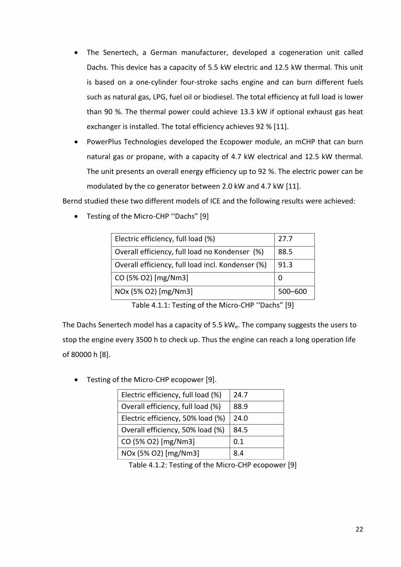
Bernd studied these two different models of ICE and the following results were achieved:

Testing of the Micro-CHP ‘‘Dachs” *9+

Table 4.1.1: Testing of the Micro-CHP ‘‘Dachs” [9]

The Dachs Senertech model has a capacity of 5.5 kWe. The company suggests the users to

stop the engine every 3500 h to check up. Thus the engine can reach a long operation life

of 80000 h [8].

Testing of the Micro-CHP ecopower [9].

Table 4.1.2: Testing of the Micro-CHP ecopower [9]

Electric efficiency, full load (%) 27.7

Overall efficiency, full load no Kondenser (%) 88.5

Overall efficiency, full load incl. Kondenser (%) 91.3

CO (5% O2) [mg/Nm3] 0

NOx (5% O2) [mg/Nm3] 500–600


Overall efficiency, full load (%) 88.9

Electric efficiency, 50% load (%) 24.0

Overall efficiency, 50% load (%) 84.5

CO (5% O2) [mg/Nm3] 0.1

NOx (5% O2) [mg/Nm3] 8.4

23

4.2 MICRO GAS TURBINE The micro gas turbines with a high capacity between 25-30 kWe and 200-250 kWe

represent a mature technology [9, 10]. This system has electric efficiency around 25%-30%

[8].

There is a substantial difference in the plant between the small-size systems and high-size

systems. The small-size systems have simple components not expensive to achieve an

optimal compromise between the costs and the efficiency. Exactly the costs are one of the

most important obstacles that limit the development of the small-size systems in the

residential sector [10].

The main components consist of generator, compressor, combustion chamber, turbine and

recuperator. The turbine is connected to each part by a shaft and the recuperator is used

to recovere the heat of exhaust gases. This device stays in an external casing.

The operation process follows the Brayton Cycle. At the beginning an external air flow

undergoes an isentropic compression by the compressor. Then the air flow runs through

heat exchanger and the combustion chamber where the air is heated. In the combustion

chamber the air is heated by fuel and the turbine subsequently expands the gases. The

exhausted gases go through the heat exchanger to recover the heat and then they are used

to heat the water which suited domestic applications.

The chemical energy of the fuel is converted into mechanical energy. A portion of this

energy is used by the compressor and the remaining energy is converted into electricity by

the generator.

The generator produces a high frequency alternating current. For this reason a rectifier and

a transformer are also needed to produce direct current for electrical devices [6].

Regarding the cogeneration system, the exhausted gases have a temperature of 200-300 °C

in the second heat exchanger and these temperatures allow to heat a water flow.

Therefore the water can achieve the temperature required for the domestic applications,

that is around 70-90 °C. At the end the gases are released in the atmosphere and their

temperature is about 100 °C [7]. If all the heat inside the gases is recovered the thermal

efficiency can achieve the value of 45-55 %. Indeed the total efficiency can reach values

around 80-90 % and the electric/power ratio is equal to 0.55-0.65 [8]. The principal fuel

burned is natural gas. It is also possible to burn other fuels as: diesel oil, gasoline,

methanol, ethanol, LPG. For instance the company Capstone produced models that are

24

able to use different fuels. The models called C30, C65 and C200 are produced in two

versions; the first version burns natural gas or LPG and the second burns biogas.

The micro gas turbine systems are very flexible in operation. They can operate in:

1. thermal follow mode. It means that the system tries to follow the thermal demand

and the electric power changes accordingly;

2. electrical follow mode. It means that the system operation is driven by the

electrical demand and the thermal power changes accordingly;

3. by-pass mode, partial or total. It means that part of the exhausted gases are directly

expelled in the atmosphere in order to limit the thermal output.

These systems are influenced by the outdoor climate conditions, especially by the air

temperature. Indeed when the air temperature increases the air density decreases and this

is the cause of the power produced reduction.

Regarding to the costs the micro gas turbine systems have a price around 1000-2000 €/kW

[7]. The manufacturers guarantee 6000-8000 hours of operation during one year. It means

that the load factor is between 70 % and 90 %. The device has an operating life of 60000-

80000 hours, corresponding to 7-8 years. However some parts have to be changed as the

combustion chamber. This piece is usually replaced every 30000 hours [8].

The payback time of the system depends on outside temperatures and operating profile. It

is between 2 and 5 years. It can achieve an economic savings around 20-25 % and CO2

savings around 6 tons per year [47].

Currently the principal companies that produce these systems are [7]:

− Capstone Turbine Corporation

− Turbec

− Elliott Energy System, Inc. (Ebara Group)

− Ingersoll Rand Company

− Bowman Power System Inc.

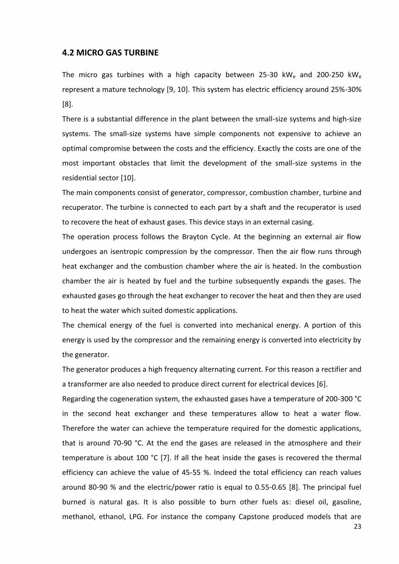
The following table resumes the most important features of some models available in the

market [7, 8].

25

Pel

[kW]

Electric

efficiency [%]

Thermal

efficiency [%]

NOx

[mg/kWhe]

CO

[mg/kWhe]

CapstoneC30

30

26 / 215 582

Ingersoll

Rand MT70

70

28 40 200 122

Bowman

TG80CG

80

26 48.8 597 /

Elliott TA80

80

28 60 555 405

Turbec T100

100

30 46.5 311 189

Table 4.2.1: features of micro gas turbine

As it can be seen the capacity is relatively high. Indeed these micro gas turbine systems are

not installed in a single family house; very well they are used in large buildings where the

thermal and electrical demand is high. For instance this solution is often installed in

hospital, airport and university.

4.3 MICRO RANKINE CYCLE (MRC) The Rankine cycle is based on an external combustion cycle [38]. The Rankine cycle

technologies are usually used to produce electricity in power generation plants. The

capacity is variable; there are small-size systems, typically few kW, and high-size systems,

typically some MW. It is possible to use the first machines in the residential sector. They

can produce the electricity and the thermal power for the heating system and domestic hot

water making available the water at the temperature of 60-90 °C [8]. The thermodynamic

cycle, when an efficient turbine is used, is similar to the Carnot cycle. The ideal cycle is

composed of a pump, a turbine, a boiler and a condenser. The working fluid enters in the

pump where it is pumped from low to high pressure. After that the high pressure liquid

enters a boiler where it is heated at constant pressure by an external heat source to

become a dry saturated vapor. The dry saturated vapor expands through a turbine,

generating power. This decreases the temperature and pressure of the vapor. The wet

vapor then enters a condenser where it is condensed at a constant pressure to become a

26

saturated liquid. The mechanical power generating by the turbine is converted into

electricity by a generator.

The working fluid is typically water, but is possible to have an organic fluid. A micro

Rankine cycle systems that use these working fluids are called organic Rankine cycle (ORC).

The organic fluid used is chosen as a function of the heat source temperature to optimize

the efficiency of the cycle [7]. Typically, refrigerants are working fluids proposed or used

for ORC systems, such as R124 (Chlorotetrafluorethane), R134a (Tetrafluoroethane) or

R245fa (Pentafluoropropane), or light hydrocarbons such as isoButane, n-Butane,

isoPentane and n-Pentane [12]. These fluids are characterized by high molecular mass.

They are dry fluids, it means that the incline of the saturated steam curve in the

thermodynamic diagram T-s is positive [7].

If the expander is a turbine, the working fluid entering must be in the dry vapor phase. This

choice is suggested to prevent blade erosion and to maintain a high efficiency [12].

Therefore the organic fluids are perfect as it is always possible to have a superheated

steam at the end of the expansion. It involves that in the turbine there is not droplets as

required. Another advantage is the possibility to decrease the expander rotational speed,

that entails a direct connection between the generator and the turbine. Furthermore the

high density of the organic fluid allows to have components with small size.

The organic fluids have a critical temperature and a critical pressure lower than the water.

It means that the operating pressure and temperature of the cycle are again lower than the

same temperature pressure if water was used as working fluid.

At the end of the expansion an organic fluid leaves the turbine like superheated steam and

it has to be cooled down and then it can enter in the condenser. Therefore the cycle can

be improved by the use of a regenerator between the turbine and the condenser. Since the

fluid has not reached the two-phase state at the end of the expansion, its temperature at

this point is higher than the condensing temperature. This higher temperature fluid can be

used to preheat the liquid before it enters the evaporator. The regenerator allows to

increase the electric efficiency but in turn also the costs increase. For this reason the

regenerator is usually used only in the systems with a high capacity. Regarding to the small-

size systems used in domestic applications with a capacity between 1 kW and 10 kW the

regenerator is not necessary as it entails an useless complication.

27

To recover the waste heat it is necessary to use a fluid. Usually this fluid is diathermic oil. In

the high-size systems the temperature of the hot source is around 800-1000 °C, while in

the small-size systems the temperature is around 300-450 °C [8].

In the residential use the boiler of the MRC systems burns natural gas, but it is possible to

have systems fed by other fuels [7].

To produce thermal power used for applications that suit domestic installations it is

necessary to heat a water flow. Therefore the water is heated in the condenser and then it

can be used in the houses heating systems. Usually the organic Rankine cycle makes

available water at the temperature between 40 °C and 60 °C [8].

In the systems with a capacity between 30 kW and 1500 kW the water is available at the

temperature of 60-90 °C. The electric efficiency is around 15-20 % and the thermal

efficiency is around 75-80 %. In these cases the total efficiency is around 90 % [7].

The small-size systems for domestic applications are available in the market but they are

not widespread. For this reason is not simple to quantify the investment and maintenance

costs and the lifetime. On the contrary the bigger systems are very widespread, therefore it

is possible to get a sense of the costs. All the system has a variable cost around 4000-6000

€/kW [7].

The company Turboden guarantees that the cogeneration plant can operate for 8000 hours

per year. The maintenance cost is around 20 €/kW per year, and if it is compared to the

producible energy, it correspond to about 0.003 €/kWh *8].

Currently the principal companies that produce these systems are [38]:

-Cogen Microsystems;

-Energetix Group plc;

-OTAG GmbH & CO KG.

The following table resumes the most important features of some available models in the

market [38, 7, 8].

28

MODELLO Potenza

elettrica [kW]

Potenza

termica [kW]

Rendimento

elettrico [%]

Rendimento

termico [%]

Cogen

Microsystems:

Small

commercial

10 44 18.5 81.4

Cogen

Microsystems:

Domestic

2.5 11 18.5 81.4

Otag Lion:

Powerblock

2 16 10.4 83.6

Genlec

(gruppo

Energetix)

Genlec

Kingston

1 8 10 80

Table 4.3.1: features micro Rankine units

For the high-size systems the undisputed leader of the market is Turboden.

4.4 STIRLING ENGINE

The ideal thermodynamic cycle is made by two isochoric transformations and two

isothermal with perfect regeneration between two isothermal transformations. This

technology is based on an external combustion engine and its simplest form the Stirling

engine comprises cylinder, regenerator, piston and displacer. Initially the working fluid is

compressed and maintained at a constant temperature, after that it passes through the

regenerator where the temperature is increased. Then it is expanded at constant

temperature. Whereupon the fluid passes back through the regenerator and arrives in the

compression-space maintaining its volume constant. It transfers heat to the regenerator

and this heat is used in the next cycle to heat the working fluid. Therefore the device

operates between two different thermal sources: the first is hot and it heats the piston

favouring the expansion process; the other is cold and removes heat by the piston,

favouring the compression process [7].

The Stirling engines present some important advantages. First of all they can operate

without valves or an ignition system, thus permitting a simple operation with low running

costs [13]. The absence of the valves and the absence of the irregular combustions allows

29

to operate without excessive noise. Strong point of these systems is the dependability due

to the absence of mechanical stresses.

If natural gas is used as a fuel the unit presents a low electrical efficiency, about 25–30 %

[2] and this is a drawback for the system.

It is possible to have two different configurations: Kinematic Stirling Engines and Free-

Piston Stirling Engines (FPSE).

To convert the reciprocal piston motion the Kinematic Stirling Engines have a crank

arrangement. Thus the reciprocal motion is convert to rotational. The Free-Piston Stirling

Engines (FPSE) is made without rotating parts. In many cases, output power is taken from a

linear alternator connected to the piston, while the displacer is controlled by the pressure

variation in the space under the piston [13]. There is another division in three typical

configurations of the displacer and working pistons, called alpha, beta and gamma. In the

first type, the working gas shuttles between two pistons. In the first piston it happens a

compression. This piston represents the cold space. The other piston, that represents the

hot space, expands the working fluid. A sub-division of the alpha type is the double-acting

type, where symmetrical pistons carry out useful work. This structure is usually chosen

because of simplicity and the facility to build the system. In the beta type in the same

cylinder the two volumes are created. Finally the last version, the gamma type, where the

working piston is set in a independent cylinder [13].

The beta type is the most efficient solution. It is even the most compact solution and the

absence of mechanical losses compensate the losses due to thermal shunt. The high

efficiency may be an advantage but it carries out economical and technical problems. So it

is necessary to have a right compromise between the costs and efficiency. However, this

device has some drawback such as variations in electrical output due to fluctuations in

rotation of the working piston. Obviously noise, vibration and mechanical stress are

increased [13].

The external combustion engine allows to choose the fuel freely. Indeed different fuels can

be burned, so this type of engine meets the favours of the people who believe in a world

driven by the renewable energy. Next to the typical fossil fuels (solid, liquid or gaseous) it is

possible to burn every type of fuel like biogas or pellet for example. Thanks to the

continuous and external combustion it is possible to have low gas emissions and noise.

30

The generated thermal power can derive from the combustion or other sources. Indeed

this system applies to the exploitation, for example, of the geothermal heat. Lately it

seems to be very interesting the Stirling engines that allow to use the solar energy, in fact

the research is concentrated in this type of devices.

In an ICE is possible to control power instantaneously thanks to the fuel supply variation.

This represents the most important difference between ICE and Stirling engines [13]. For

this reason ICE is the ideal engine to supply rapid variations in power, required for example

for automotive applications. In a Stirling engine the warm up time is greater than in a ICE.

However the engine continues to transfer energy to the working gas even if it is off due to

heat stored in the hot end. This problem is not taken into account in stationary applications

where instantaneous power variation is not required. It is worth mentioning that there is a

delay between a thermostat calling for heat and the output of power [13]. This delay will

be of the order of minutes.

The commercial systems that present an electrical capacity lower than 10 kW are mostly

prototypes. The range of the electric power is from 1 kW to 9 kW, while the range of the

thermal power is from 5 kW to 25 kW. These prototypes represent a good alternative to

conventional heating systems. The electric efficiency is between 13 % and 28 %. The total

efficiency can achieve value higher than 80 % [10].

Currently the principal companies that produce these systems for residential applications

are [41]:

WhisperGen;

MEC (Microgen);

Infinia (STC);

Disenco (Inspirit).

The Disenco develops a beta type engine with an electric capacity of 3 kW and a thermal

power can vary between 12 kW and 18 kW. The total efficiency can achieve the value of 92

% and the company guarantees a lifetime of 15 years [11, 41].

The Infinia produces a liner free piston Stirling engine used for co generative applications in

a single dwelling. This system has an electric capacity of 1 kW , while the thermal capacity

31

is 6.4 kW. The electric efficiency is 12.5 %, while the thermal efficiency is 80 %. Regarding

to the costs of the model the supply only cost in the UK market is 6000-8000 £ related to

2010 [11, 41].

The MICROGEN develops a liner free piston Stirling engine characterized by high

performances, absence of noise and high dependability [41]. It contains a auxiliary burner

to cover the heat demand in each solution, even larger homes. It has an electric capacity

of 1 kW and thermal capacity of 6 kW. The electric and thermal efficiency are respectively

13.5 % and 81.1 %. The supplementary burner has a capacity between 18 kWt and 28 kWt.

Regarding to the costs of the model the supply only cost in the NL market of 10000 € and

installed costs in UK about 6000-8000 £ related to 2010. This unit can be considered the

most efficient and dependable engines available in the market [11, 41].

The WhisperGen micro CHP unit is marketed in the UK by energy company, E.ON (formerly

Powergen). It is a four cylinder unit which leads to smooth, low vibration operation, and

low noise. The Mk5 unit, incorporating an auxiliary burner, was introduced to give more

flexibility. Thus the unit can meet the full heating requirements for even larger homes. It

has an electric capacity of 1 kW, while the thermal capacity is 7 kW. The supplementary

burner has a capacity of 5 kWt. Regarding to the costs they depend on the country. For

example the supply only cost in Germany is around 10000 €; the installed cost in UK was

3000 £ in 2004, while in 2010 was 6000-8000 £. The seam cost during the seam year in

Germany was 14,000 € [11, 41].

It is interesting to show the result of the Bernd Thomas’ study. The performance of SOLO

Stirling 161 and Micro-CHP SM5A were investigated.

The first unit incorporates a 2-cylinder Stirling engine in alpha-configuration, with an

electric output ranges from 2 kW to 9 kW and thermal output ranges from 8 kW to 26 kW

[9]. The follow table summarize the model performance.



Electric efficiency, 50% load (%) 24.8

Overall efficiency, 50% load (%) 95.1

CO (5% O2) [mg/Nm3] 191

NOx (5% O2) [mg/Nm3] 105

Table 4.4.1: Testing of the Micro-CHP SOLO Stirling 161 [9]

32

The second unit was developed at the Danish Technical University (DTU). The unit was

driven by natural gas on the test stand. The Stirling engine studied in [9] was a beta-type

engine. The unit had an electric capacity of 9 kW corresponding to a thermal power of 25

kW. The follow table summarize the model performance.



CO (5% O2) [mg/Nm3] 154

NOx (5% O2) [mg/Nm3] 365

Table 4.4.2: Testing of the Micro-CHP SM5A [9]

The Stirling engines technologies is not frequently installed as said in [11]. But in the next

feature they will increase because of their advantages, such as global efficiency, fuel

flexibility low emission level, low vibration and noise level [11].

33

5 CURRENT STATES OF INVESTIGATIONS

It is worth mentioning also the technologies not mature and not available in the market.

Researchers are studying these systems to develop models suitable for domestic

application that cover the electric and thermal demand. Afterwards it will be discussed the

following systems:

1. Termophotovoltaic systems;

2. Fuel cell systems.

5.1 SISTEMA TERMOFOTOVOLTAICO TPV The termophotovoltaic (TPV) system is a technology who allows to generate electricity

through photovoltaic cells. These cells are particularly sensitive to infra-red radiation. The

radiation is radiated by a device that achieves the emission temperature thanks to a

burner.

The system operates through boiler, which use a surface radiant burner. Inside the

combustion chamber of this boiler takes place a controlled combustion. The surface emits

radiation mainly infrared when it reaches the operating temperature. The radiation is

filtered and then it arrives at the cells sensitive to this wavelength.

The photovoltaic cells carry out an important task. They convert the incident radiation into

electricity.

The principal components of the TPV systems are: heat source, thermal emitter, optical

filter that controls the spectrum of the emitted radiation and photovoltaic cells [7].

The filter has an important function. It has to protect the cells by the combustion gases as

well as control the spectrum of the radiations. The type of the heat sources used depend

on the thermal emitter.

The TPV systems can be divided in two different groups: the first family consists of the

external combustion systems, the second consists of the internal combustion systems [8].

In the external combustion units the thermal emitter consists of a closed combustion

chamber, where the exhausted gases do not come in contact with the photovoltaic cells.

They remain inside the chamber and they brush the internal surface. In this case it can be

used the traditional fuels such as natural gas or diesel oil, fuels from renewable sources like

34

biomass, biogas or syngas, other generic sources of heat such as waste heat of industrial

processes or heat resulting from solar concentrators [8].

In the internal combustion systems the exhausted gases come in contact with the space

where the cells are positioned. The emitter consists of a porous burner. In this case the

emitter achieve the operating temperature through the heat exchanged between the

exhausted gases of the combustion and the porous matrix. Unlike the external combustion

systems in these units the fuels used are gaseous fuels medium-high quality.

The materials that composed the photovoltaic cells are Silicon (Si) and Germanium (Ge).

These materials are inexpensive, but they are the drawback to have a high activation

energy, not suited for these applications. It is possible to use other materials such as

Gallium (Ga), Antimony (Sb), indium (In) and Arsenic (As). They have an activation energy

lower than the previous materials, farther they are more efficient. There are two

drawback: first and foremost Antimony and Arsenic are toxic, then the costs to produce

these elements are high.

A typical TPV system used for co-generation applications consists of a boiler that heats a

burner. The burner is the emitter and it is surrounded by the photovoltaic cells.

The unit operates by a thermal follow mode because the principal function is cover the

thermal demand of the house. The hot gases produced by the systems heat the water

required for space heating and DHW. On the contrary the electricity is a by-product.

All heat not converted into electric energy by the PV cells can be recovered. Although the

electric efficiency of TPV CHP systems range from 2 % to 5 %. These values are relative to

available prototypes. However the total efficiency is always higher than 90 % and can

achieve 100 % if it is used devices that recover of condensation heat [8, 10].

The TPV systems are very versatile due to different size. Researchers are studying units

with a capacity around 1-2 W [7]. These small systems are used for applications in

electronic sector. It is worth mentioning devices with a capacity between 100 W and 300 W

that produce energy in vehicles such as recreational vehicles [42]. The units for domestic

co-generation applications have a capacity of 1000-3000 W, similar to the capacity of the

other mCHP systems described above [7, 8].

Nowadays the TPV systems are being developed and there are only prototypes. The

company JX Crytal produce a model called Midnight Sun and it is sold about 10 units. This

model has a capacity of 7.3 kWt. The material the composes the cell is Ga-Sb. The model

35

can generate 100 We necessary to its self-sustaining. The surplus can be used to recharge

batteries. The production has been abandoned, and the company is developing a non

commercial model with a thermal power of 12.2 kW and electric capacity of 1.5 kW [8].

The Paul Scherrer Institute developed a system with a capacity between 12 kWth and 20

kWth. It has an electric capacity around 100-200 W ant the electric efficiency is about 1 %.

Furthermore the institute developed prototypes used like portable systems with capacity

of 30 We and 50 We. The electric efficiency is between 1.5 % and 2.5 % [7, 8].

Another institute interested and active in this field is CANMET Energy Technology Centre.

Nowadays only prototypes are studied.

Regarding the costs it is not simple have an idea because there are not available

commercial systems. However in literature it is possible to find the following costs

regarding some prototypes studied [7].

Modello Costo

Midnight Sun /

JX Crystal

(caldaia+TPV)

5250 €

(3500 €/kW)

JX Crystal

(solo TPV)

800 €

(1800 €/kW)

Paul Scherrer

Inst

590 €

(2950 €/kW)

Table 5.1.1: TPV costs

These systems have several advantages. First of all it is possible to use different fuels.

Second of all they have high total efficiency [8]. Inside the device there are no moving

parts, therefore there is no noise and it does not need to emergency maintenance [7].

Furthermore the costs are not too much high and comparable with other mCHP

technologies. Finally there are environmental advantages due to the reduction of gases

emissions such as CO and NOx, more than the other co-generation systems [8].

The highest problem of this technology is the electric efficiency. Thus researchers try to

focus on improving the efficiency of TPV. It is worth mentioning a particularly promising

technology, called DRAX burner, where the emitter will achieve a higher temperature. In

this case it will emit more of the near infra-red and visible radiation that the photovoltaic

cells require [42].

36

5.2 CELLE A COMBUSTIBILE FC

The fuel cell is a new particular interesting technology. It can be used for residential co-

generative applications or to produce electricity.

Usually a fuel cell system is made by some cells in parallel to achieve the desired size. The

unit is called stack.

Inside the fuel cells there is no combustion. Indeed this device converts the chemical

energy from a fuel into electricity through a chemical reaction. The structure of the fuel cell

is very simple. It consists of a positive side, called cathode, and a negative side, called

anode. Furthermore an electrolyte is interposed between the two electrodes. Even if there

is no combustion the systems need a fuel and a combustive agent. The fuel enters in the

negative side, while the combustive agent enters in the positive side. Inside the fuel cell

two semi-reactions occur:

1. oxygen reduction reaction

2. hydrogen oxidation reaction

Electrons are released by the anode which reach the positive side through an external

circuit. Ions diffuse from the anode to the cathode through the electrolyte and after that

they are converted into water by the oxygen reduction reaction. The rapidity of the process

depend on catalysts. Indeed there are anode and cathode catalysts that promote the

reactions.

The reactions release electrons in the negative side and they generate direct current. Thus

the systems can feed an external load. The principal fuel utilized by the fuel cell is the H2.

In literature there are several types of fuel cells. Here only five major types of fuel cells is

reported according to [43]. They are diversified to each other on the basis of their

electrolyte [43]:

Phosphoric acid fuel cell, PAFC;

Polymer electrolyte membrane fuel cell, PEMFC;

Alkaline fuel cell, AFC;

Molten carbonate fuel cell, MCFC;

Solid oxide fuel cell, SOFC;

37

Taking into account the operating temperature it is possible divide the systems in two

groups:

1. high temperature fuel cell (MCFC and SOFC);

2. low temperature fuel cell (AFC,PEMFC, PAFC).

The following table summarizes the principal features of the systems [2, 8, 43].

PAFC PEMFC AFC MCFC SOFC

Electrical efficiency [%]

40 40-50 50 45-55 50-60

Power range [kW]

50-1000 0.001-1000 1-100 100-100000 10-100000

Internal Reforming

NO NO NO YES YES

Electrolyte

Phosphoric acid

Polymeric membrane

Potassium hydroxide

Nitrate, sulphate

or carbonate in molten

condition

Solid ceramic material

Operational temperature [°C]

150-210 60-110 90-250 600-700 700-1000

Oxidant Air Air O2 Air Air

Table 5.2.1: principal features of fuel cells The system is composed of: the fuel cell strack (fuel cell subsystem), where is produced the

electric energy like direct current (DC); the thermal management subsystem who takes

over the management of cooling requirements; the fuel delivery-processing subsystem

who includes the hydrogen storage system or the internal reforming system. Latter is a

chemical reactor where is generated hydrogen by other fuels; the power electronics

subsystem where the direct current, provided by stack, is converted in alternating current.

The fuel cells seem to have a lot of advantages. The most important advantage is the very

low emission rate; if they use a reforming process they produce CO2 and other emissions, if

they use pure hydrogen the output is only water. On the other hand current prototypes

have a lot of drawbacks. They are too noisy, bulky, inefficient and they have high initial cost

[13].

38

Not all the systems are used for the same applications. For example the PEMFC and the

DMFC appear suited for portable power application because of they have low operating

temperature and high energy/power density.

The heat produced by the fuel cell during its operation can be recovered and used for co

generative applications. The two most interesting models of fuel cell systems being

developed for micro CHP applications are PEMFC and SOFC [44].

PEM fuel cell will install for residential cogeneration systems. It is due to its optimal

performances in converting the heat of the exhausted gases into useful energy. Thus it can

use usefully all the waste heat generated from the electricity process. This thermal power

is used to meet both thermal demands for space heating and hot domestic water in the

residential sector [14]. On the other hand this technology presents a low operating

temperature. It is a problem in domestic CHP applications, because the unit could not

achieve the hot water operating temperature. Therefore SOFC fuel cells seem to be more

attractive in domestic CHP applications, not only for the operating temperature, but also

for higher potential electrical efficiency of SOFC units [44]. Both these technologies can be

used in standalone houses, or in parallel with the grid.

There are some prototypes and below are shown few main characteristics [44].

MODEL FC TYPE POWER ELECTRICAL EFFICIENCY [%]

AVAILABILITY COST [€]

Toshiba PEM 700 kWe 40 Japan 2011 Europe 2015?

25000

Elcore PEM 300We; 600Wt 30 2012 Field trials in Germany

2013 Proposed market launch

in Germany

9000 installed

Baxi Innotech

PEM 1kWe : 1.7-20kWt

32 Field Trials in Germany & UK

/

Ceramic Fuel Cells

SOFC Bluegen (DHW plus power)

1.5kWe; 600Wt Micro CHP

1.0kWe: 0.3kWt

/ Bluegen 1.5kWe available now in

UK, NL, DE. Packaged micro

CHP version field trial 2012

Bluegen 25000

Table 5.2.2: mian available prototypes

http://www.elcore2400.com/home.html

http://www.baxitech.co.uk/Baxi_Tech/BaxiTechWeb.nsf/index.html

http://www.baxitech.co.uk/Baxi_Tech/BaxiTechWeb.nsf/index.html

http://www.cfcl.com.au/html/product.htm

http://www.cfcl.com.au/html/product.htm

39

Nowadays fuel cells is not still mature and the high price of this technology is greater than

the costs of other micro CHP technologies.

40

6 THEORETICAL BACKGROUND OF MODELLING SOFTWARE

Energy Plus is a free software. It is composed of different modules. These modules,

working together, can evaluate the energy required for heating and cooling necessary to

obtain the comfort conditions for the domestic application at all the time steps. The

program manages: surface heat balance, air heat balance and building system simulation

and these simulations depend on several modules. The program solves simultaneously

three principal parts, that consist of building, system, and plant. To solve the resulting

ordinary differential equations Energy Plus uses a predictor-corrector approach.

The core of the simulation is a heat balance equation on the zone air [36]:

𝐶𝑧 𝑑𝑇𝑧

𝑑𝑇= 𝑄𝑖 + ℎ𝑖 𝐴𝑖 𝑇𝑠𝑖 − 𝑇𝑧

+

𝑁𝑠𝑢𝑟𝑓

𝑖=1

𝑚𝑖 𝐶𝑝 (𝑇𝑧𝑖

− 𝑇𝑧 )

𝑁𝑧𝑜𝑛𝑒𝑠

𝑖=1

𝑁𝑠𝑙

𝑖=1

+

+ 𝑚𝑖𝑛𝑓 𝐶𝑝 𝑇∞ − 𝑇𝑧 + 𝑄𝑠𝑦𝑠 (Eq 6.1)

Where:

𝑄𝑖 =𝑁𝑠𝑙𝑖=1 sum of the convective internal loads;

𝐶𝑧 𝑑𝑇𝑧

𝑑𝑇 = energy stored in zone air;

ℎ𝑖 𝐴𝑖 𝑇𝑠𝑖 − 𝑇𝑧 𝑁𝑠𝑢𝑟𝑓

𝑖=1 = convective heat transfer from the zone surfaces;

𝑚𝑖𝑛𝑓 𝐶𝑝 𝑇∞ − 𝑇𝑧 = heat transfer due to infiltration of outside air;

𝑚𝑖 𝐶𝑝 (𝑇𝑧𝑖 − 𝑇𝑧 )𝑁𝑧𝑜𝑛𝑒𝑠𝑖=1 = heat transfer due to interzone air mixing;

Q

sys = air systems output;

Cz = ρair Cp CT;

ρair = zone air density;

Cp = zone air specific heat;

CT = sensible heat capacity multiplier.

In order to have a simulation that is physically realistic, the integrated solution manager

connects all the elements in a simultaneous solution scheme. To simplify the description of

the entire integrated program it is possible to guess a series of functional elements

connected by fluid loops. Therefore the first part, the zone, is linked to the system by an air

loop and the second part is linked to the plant by a water loop. The program required that

the temperature of the water entering the coils is equal to the temperature leaving the

chillers or boilers; the temperature of the return water from the coils is the same as the

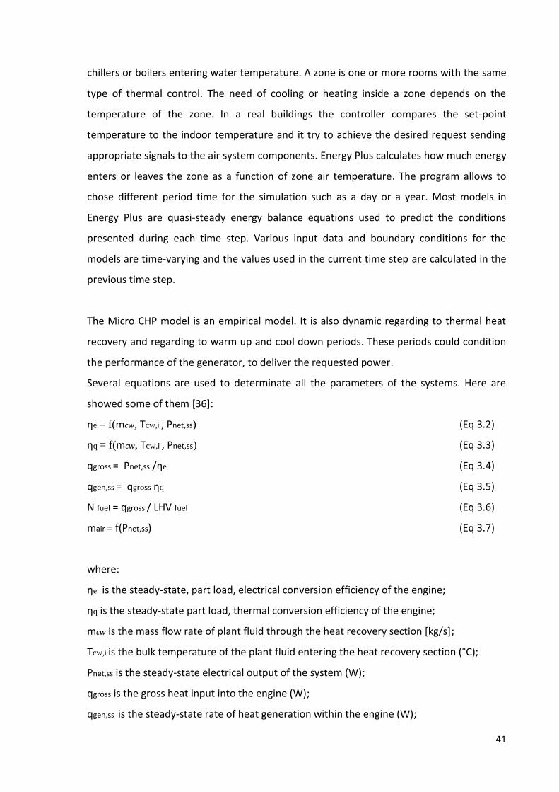
41

chillers or boilers entering water temperature. A zone is one or more rooms with the same

type of thermal control. The need of cooling or heating inside a zone depends on the

temperature of the zone. In a real buildings the controller compares the set-point

temperature to the indoor temperature and it try to achieve the desired request sending

appropriate signals to the air system components. Energy Plus calculates how much energy

enters or leaves the zone as a function of zone air temperature. The program allows to

chose different period time for the simulation such as a day or a year. Most models in

Energy Plus are quasi-steady energy balance equations used to predict the conditions

presented during each time step. Various input data and boundary conditions for the

models are time-varying and the values used in the current time step are calculated in the

previous time step.

The Micro CHP model is an empirical model. It is also dynamic regarding to thermal heat

recovery and regarding to warm up and cool down periods. These periods could condition

the performance of the generator, to deliver the requested power.

Several equations are used to determinate all the parameters of the systems. Here are

showed some of them [36]:

ηe = f(mcw, Tcw,i , Pnet,ss) (Eq 3.2)

ηq = f(mcw, Tcw,i , Pnet,ss) (Eq 3.3)

qgross = Pnet,ss /ηe (Eq 3.4)

qgen,ss = qgross ηq (Eq 3.5)

N fuel = qgross / LHV fuel (Eq 3.6)

mair = f(Pnet,ss) (Eq 3.7)

where:

ηe is the steady-state, part load, electrical conversion efficiency of the engine;

ηq is the steady-state part load, thermal conversion efficiency of the engine;

mcw is the mass flow rate of plant fluid through the heat recovery section [kg/s];

Tcw,i is the bulk temperature of the plant fluid entering the heat recovery section (°C);

Pnet,ss is the steady-state electrical output of the system (W);

qgross is the gross heat input into the engine (W);

qgen,ss is the steady-state rate of heat generation within the engine (W);

42

LHV fuel is the lower heating value of the fuel used by the system (J/kg or J/kmol);

N fuel is the molar fuel flow rate (kmol/s);

mair is the mass flow rate of air thru the engine (kg/s).

43

7 DWELLING DESCRIPTION

The modelling of the house presupposed to know the construction details, the

characteristics of the family that lives in the building, electrical thermal and space heating

demand.

Two different operating mode were taken into account for mCHP prime mover and

compared with a reference scenario:

1. the generation of space heating by means of mCHP system plus an auxiliary boiler

with gas fired boiler for DHW;

2. the DHW heat generation by means of mCHP system that heated a water tank for

one hour during the morning and then, with an auxiliary boiler, covered the space

heating demand.

7.1 DOMESTIC AND OCCUPANCY CHARACTERISTICS

The building studied was a detached three floors detached house. The dwelling is located

in the north east of Italy, to be more precise in Caerano di san Marco, in the climate zone E.

The floor area is 340 m², but only 240 m² is heated corresponding to the zero floor and the

first floor. The basement has a floor height of 2.4 m, while the other two floor has a height

of 2.7 m. The house has a 46 m² glazing. It was modelled with six individual energy zones.

Figure 7.1.1: design of single house

44

In the following tables illustrate the construction details.

Exterior Floor Thickness

(m)

Conductivity

(W/mK)

Density

(kg/m³)

Specific Heat

(J/kgK)

concrete sand 0.04 1.081 1800 880

internal cardboard bitumen 0.01 0.186 1100 1410

concrete clay 0.08 0.4 800 920

lean concrete 0.04 0.93 2000 840

marble floor 0.025 3.37 3700 840

Table 7.1.1: Exterior floor construction details

Interior Floor Thickness

(m)

Conductivity

(W/mK)

Density

(kg/m³)

Specific Heat

(J/kgK)

interior plaster 0.015 0.697 1800 840

loft 0.2 0.53 730 840

concrete sand 0.04 1.081 1800 880


lean concrete 0.04 0.93 2000 840

wood floor 0.025 0.2 800 2000

Table 7.1.2: Interior floor construction details

Interior Ceiling Thickness

(m)

Conductivity

(W/mK)

Density

(kg/m³)

Specific Heat

(J/kgK)

loft 0.2 0.53 730 840

concrete sand 0.04 1.081 1800 880


lean concrete 0.04 0.93 2000 840

wood floor 0.025 0.2 800 2000

Table 7.1.3: Interior Ceiling construction details

45

Exterior Wall Thickness (m) Conductivity

(W/mK)

Density

(kg/m³)

Specific Heat

(J/kgK)

exterior plaster 0.015 1.4 2000 840

brick 0.18 0.523 1200 840

insulation 0.05 0.039 25 1250

internal brik 0.08 0.418 800 840


Table 7.1.4: Exterior wall construction details

Interior Wall Thickness (m) Conductivity

(W/mK)

Density

(kg/m³)

Specific Heat

(J/kgK)

plaster 0.01 0.697 1800 840

internal brik 0.08 0.418 800 840

plaster 0.01 0.697 1800 840

Table 7.1.5: Interior wall construction details

Exterior Roof Thickness

(m)

Conductivity

(W/mK)

Density

(kg/m³)

Specific

Heat (J/kgK)

external cardboard bitumen 0.001 0.23 1200 1410

fir 0.022 0.12 450 2000

polystyrene 0.05 0.042 30 1250

fir 0.022 0.12 450 2000

internal cardboard bitumen 0.01 0.186 1100 1410

Table 7.1.6: Exterior roof construction details

46

BasementWall Thickness (m) Conductivity

(W/mK)

Density

(kg/m³)

Specific

Heat (J/kgK)

exterior plaster 0.015 1.4 2000 840

reinforced concrete 0.08 1.511 2400 840

expanded polystyrene 0.05 0.039 25 1250

reinforced concrete 0.08 1.511 2400 840


Table 7.1.7: Basement wall construction details

The house is inhabited by five people, one of the parents works in the morning, other

parent works all the day, then there are school attending children. The energy

consumption depends on the presence of the inhabitants inside the dwelling. Regarding

the space heating schedule was assumed to be no difference between a typical weekday

and weekend day. The heating system was assumed to be on in the evening, from 19:00 to

23:00, therefore during this period the boiler or mCHP system had to cover the thermal

demand. The bills was checked and the total annual gas consumption was 23602 kWh.

Regarding the electrical demand the annual consumption was 3518 kWh and this value is

in accordance to the Italian consumption [29, 45]. Two design days were taken into

account. In this case the electrical load distribution during a weekday was different from

weekend day as it is possible to see in the following tables.

0

0,1

0,2

0,3

0,4

0,5

0,6

0,7

0,8

00

.15

.00

10

.15

.00

20

.15

.00

00

.00

.00

kWh

e

47

Figure 7.1.2: electrical load distribution in a typical weekday

Figure 7.1.3: electrical load distribution in a typical weekend day

In the weekday the electrical demand is concentrated in the evening due to the

characteristics of the inhabitants. In this case the peak value is 0.6675 kWhe grater than the

weekend day value equal to 0.5975 kWhe. In the weekend day the load is more distributed

and the daily consumption is 10.47 kWhe, while in the weekday is 10.92 kWhe.

Only four of the six zones modelled was heated with a convection space heating system.

These zone are kitchen, study-room and lounge in the zero floor, and second floor. In the

reference scenario the temperature was set at 18 °C, while in the mCHP simulations the set

point temperature was fixed at 21 °C. The domestic hot water demand was covered by a

water tank with a capacity of 95 L. As reported in [31] the dhw daily consumption is 50

L/person. Therefore the total daily consumption was 250 L. In the reference scenario the

dhw was heated by gas fired boiler. In accordance with [32] for the water tank was

assumed heat losses of 0.843 W/K. The set point temperature inside the water tank was 75

°C. The boiler that heated the water was switched off if the temperature was between 75

°C and 69 °C. If the temperature dropped by 6 °C the system was modelled to heat the

water. The dhw circuit is presented in APPENDIX I.

0

0,1

0,2

0,3

0,4

0,5

0,6

0,7

00

.15

.00

02

.15

.00

04

.15

.00

06

.15

.00

08

.15

.00

10

.15

.00

12

.15

.00

14

.15

.00

16

.15

.00

18

.15

.00

20

.15

.00

22

.15

.00

kWh

e

48

In the next chapter different solutions of heating systems are presented. It is worth

showing the annual temperature profile in the four active zone if no space hating was

applied. The follow graph reports the profiles.

Figure 7.1.4: temperature zones profile with no heating systems

As showed, the study room and lounge profiles are overlapping. The higher temperature

was in the first floor during the summer, and the lower also in the first floor. The kitchen

presented the grater temperature during the winter

-5

0

5

10

15

20

25

30

35

12

67

53

37

99

10

65

13

31

15

97

18

63

21

29

23

95

26

61

29

27

31

93

34

59

37

25

39

91

42

57

45

23

47

89

50

55

53

21

55

87

58

53

61

19

63

85

66

51

69

17

71

83

74

49

77

15

79

81

82

47

85

13

[°C]

KITCHEN:Zone/Sys Air Temperature [C](Hourly)STUDY_ROOM:Zone/Sys Air Temperature [C](Hourly)LOUNGE:Zone/Sys Air Temperature [C](Hourly)FIRST_FLOOR:Zone/Sys Air Temperature [C](Hourly)

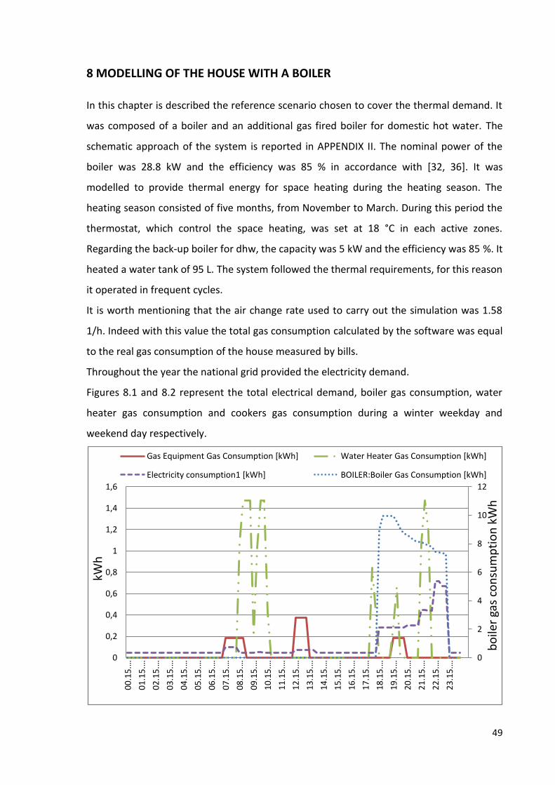
49

8 MODELLING OF THE HOUSE WITH A BOILER

In this chapter is described the reference scenario chosen to cover the thermal demand. It

was composed of a boiler and an additional gas fired boiler for domestic hot water. The

schematic approach of the system is reported in APPENDIX II. The nominal power of the

boiler was 28.8 kW and the efficiency was 85 % in accordance with [32, 36]. It was

modelled to provide thermal energy for space heating during the heating season. The

heating season consisted of five months, from November to March. During this period the

thermostat, which control the space heating, was set at 18 °C in each active zones.

Regarding the back-up boiler for dhw, the capacity was 5 kW and the efficiency was 85 %. It

heated a water tank of 95 L. The system followed the thermal requirements, for this reason

it operated in frequent cycles.

It is worth mentioning that the air change rate used to carry out the simulation was 1.58

1/h. Indeed with this value the total gas consumption calculated by the software was equal

to the real gas consumption of the house measured by bills.

Throughout the year the national grid provided the electricity demand.

Figures 8.1 and 8.2 represent the total electrical demand, boiler gas consumption, water

heater gas consumption and cookers gas consumption during a winter weekday and

weekend day respectively.

0

2

4

6

8

10

12

0

0,2

0,4

0,6

0,8

1

1,2

1,4

1,6

00

.15

.…

01

.15

.…

02

.15

.…

03

.15

.…

04

.15

.…

05

.15

.…

06

.15

.…

07

.15

.…

08

.15

.…

09

.15

.…

10

.15

.…

11

.15

.…

12

.15

.…

13

.15

.…

14

.15

.…

15

.15

.…

16

.15

.…

17

.15

.…

18

.15

.…

19

.15

.…

20

.15

.…

21

.15

.…

22

.15

.…

23

.15

.…

bo

iler

gas

con

sum

pti

on

kW

h

kWh

Gas Equipment Gas Consumption [kWh] Water Heater Gas Consumption [kWh]

Electricity consumption1 [kWh] BOILER:Boiler Gas Consumption [kWh]

50

Figure 8.1: weekday electrical demand, boiler gas consumption, water heater gas

consumption, cookers gas consumption profile

Figure 8.2: weekend day electrical demand, boiler gas consumption, water heater gas

consumption, cookers gas consumption profile

As it is possible to see, there are two ordinate axes in the figure. This is due to compare

different profiles and make readable the figures. Therefore the axis on the right

correspond to the boiler gas consumption, the axis on the left correspond to the other

profiles. The graphs show as the water heater gas consumption and electrical demand

profiles are different. On the other hand boiler gas consumption cookers gas consumption

profiles are the same during a weekend day and weekday. Regarding the dhw, figure 8.3

and 8.4 show the dhw demand compared to the dhw gas consumption during a winter

weekday and weekend day respectively.

0

2

4

6

8

10

12

0

0,2

0,4

0,6

0,8

1

1,2

1,4

1,6

00

.15

.…

01

.15

.…

02

.15

.…

03

.15

.…

04

.15

.…

05

.15

.…

06

.15

.…

07

.15

.…

08

.15

.…

09

.15

.…

10

.15

.…

11

.15

.…

12

.15

.…

13

.15

.…

14

.15

.…

15

.15

.…

16

.15

.…

17

.15

.…

18

.15

.…

19

.15

.…

20

.15

.…

21

.15

.…

22

.15

.…

23

.15

.…

bo

iler

gas

con

sum

pti

on

kW

h

kWh

Gas Equipment Gas Consumption [kWh] Water Heater Gas Consumption [kWh]

Electricity consumption [kWh] BOILER:Boiler Gas Consumption [kWh]

51

Figure 8.3: DHW during weekday

Figure 8.4: DHW during weekend day

Both simulations the back-up boiler was frequently switched on and off to supply the dhw

demand, as it is possible to see in the figures.

It is worth reporting the temperature profile for the four zone. In the figure 8.4 is also

reported the thermal power of the boiler.

0

5

10

15

20

25

30

35

40

45

0

0,2

0,4

0,6

0,8

1

1,2

1,4

1,6

00

.15

.00

01

.15

.00

02

.15

.00

03

.15

.00

04

.15

.00

05

.15

.00

06

.15

.00

07

.15

.00

08

.15

.00

09

.15

.00

10

.15

.00

11

.15

.00

12

.15

.00

13

.15

.00

14

.15

.00

15

.15

.00

16

.15

.00

17

.15

.00

18

.15

.00

19

.15

.00

20

.15

.00

21

.15

.00

22

.15

.00

23

.15

.00

Litr

es

kWh

Water Heater Gas Consumption [kWh] Dhw demand [L]

0

5

10

15

20

25

30

35

40

45

0

0,2

0,4

0,6

0,8

1

1,2

1,4

1,6

00

.15

.00

01

.15

.00

02

.15

.00

03

.15

.00

04

.15

.00

05

.15

.00

06

.15

.00

07

.15

.00

08

.15

.00

09

.15

.00

10

.15

.00

11

.15

.00

12

.15

.00

13

.15

.00

14

.15

.00

15

.15

.00

16

.15

.00

17

.15

.00

18

.15

.00

19

.15

.00

20

.15

.00

21

.15

.00

22

.15

.00

23

.15

.00

Litr

es

kWh

Water Heater Gas Consumption [kWh] Dhw demand [L]

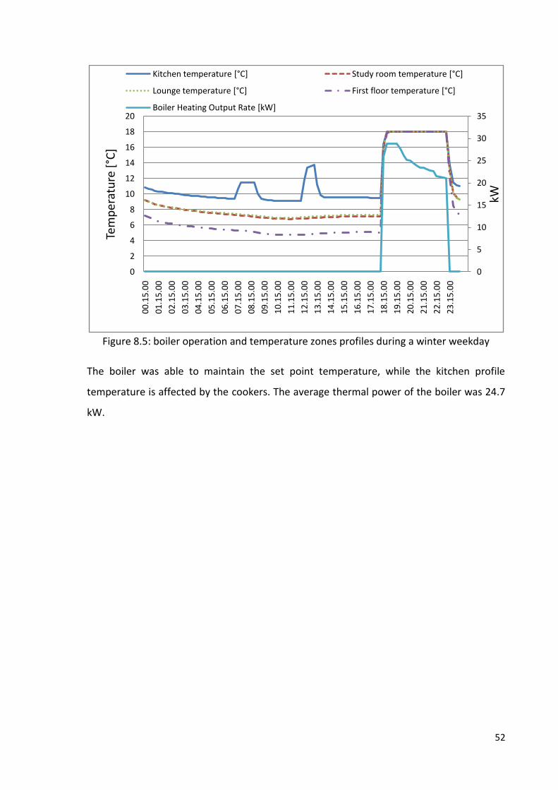
52

Figure 8.5: boiler operation and temperature zones profiles during a winter weekday

The boiler was able to maintain the set point temperature, while the kitchen profile

temperature is affected by the cookers. The average thermal power of the boiler was 24.7

kW.

0

5

10

15

20

25

30

35

0

2

4

6

8

10

12

14

16

18

20

00

.15

.00

01

.15

.00

02

.15

.00

03

.15

.00

04

.15

.00

05

.15

.00

06

.15

.00

07

.15

.00

08

.15

.00

09

.15

.00

10

.15

.00

11

.15

.00

12

.15

.00

13

.15

.00

14

.15

.00

15

.15

.00

16

.15

.00

17

.15

.00

18

.15

.00

19

.15

.00

20

.15

.00

21

.15

.00

22

.15

.00

23

.15

.00

kW

Tem

per

atu

re [

°C]

Kitchen temperature [°C] Study room temperature [°C]

Lounge temperature [°C] First floor temperature [°C]

Boiler Heating Output Rate [kW]

53

9 MODELLING OF THE HOUSE WITH INTERNAL COMBUSTION ENGINE

9.1 INTERNAL COMBUSTION ENGINE PLUS AUXILIARY BOILER WITH GAS FIRED BOILER FOR

DHW

The thermal power required for the space heating was produced by an internal combustion

engine plus an auxiliary boiler. This was due to the low power output of the mCHP unit,

which was not able to supply the demand during the coldest days. For this reason the

engine was coupled with boiler. The thermal output of the boiler was 20 kW and the

efficiency was 85 %. Regarding the ICE, was installed Dachs mCHP unit, manufacture by

SenerTec. The schematic approach is illustrated in APPENDIX III. The circuit shows as boiler

and mCHP unit were in parallel.

As technical specifications was used the default settings that is possible to find in Energy

Plus. These values are in accordance with [11]. The unit had a rated electric power output

of 5.5 kW, a rated thermal to electrical power ratio of 2.444. The electric and thermal

efficiency was respectively of 27 % and 66 %. Concerning the dhw the same buck-up boiler

modelled for the reference scenario was used for dhw in this simulation.

As state above the set point temperature was increased from 18 °C to 21 °C. This choice is

in agree with [30]. The heating season and daily schedule were the same used in the

previous configuration.

The mCHP unit produced electricity and it was used on site. The surplus fed the grid.

During the peak time, when the demand is over than the output, the electrical grid

provided to cover the requests. The follow figures illustrate the total gas consumption

profiles for the space heating, composed of boiler gas consumption, mCHP gas

consumption. Then it is drawn the operating characteristic of mCHP and boiler. The

cookers were controlled by the same schedule that controlled the reference scenario. For

this reason their profile is not reported.

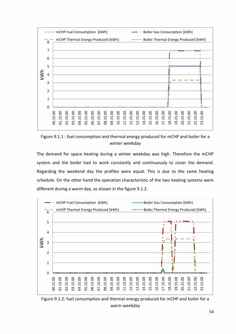
54

Figure 9.1.1 : fuel consumption and thermal energy produced for mCHP and boiler for a

winter weekday

The demand for space heating during a winter weekday was high. Therefore the mCHP

system and the boiler had to work constantly and continuously to cover the demand.

Regarding the weekend day the profiles were equal. This is due to the same heating

schedule. On the other hand the operation characteristic of the two heating systems were

different during a warm day, as shown in the figure 9.1.2.


warm weekday

0

1

2

3

4

5

6

7

8

00

.15

.00

01

.15

.00

02

.15

.00

03

.15

.00

04

.15

.00

05

.15

.00

06

.15

.00

07

.15

.00

08

.15

.00

09

.15

.00

10

.15

.00

11

.15

.00

12

.15

.00

13

.15

.00

14

.15

.00

15

.15

.00

16

.15

.00

17

.15

.00

18

.15

.00

19

.15

.00

20

.15

.00

21

.15

.00

22

.15

.00

23

.15

.00

kWh

mCHP Fuel Consumption [kWh] Boiler Gas Consumption [kWh]

mCHP Thermal Energy Produced [kWh] Boiler Thermal Energy Produced [kWh]

0

1

2

3

4

5

6

00

.15

.00

01

.15

.00

02

.15

.00

03

.15

.00

04

.15

.00

05

.15

.00

06

.15

.00

07

.15

.00

08

.15

.00

09

.15

.00

10

.15

.00

11

.15

.00

12

.15

.00

13

.15

.00

14

.15

.00

15

.15

.00

16

.15

.00

17

.15

.00

18

.15

.00

19

.15

.00

20

.15

.00

21

.15

.00

22

.15

.00

23

.15

.00

kWh



55

The operation of the boiler and mCHP during a warm day was different if it is compared to

the operation during a cold day. In a warm day the mCHP unit was able to cover almost all

the thermal demand. Moreover the system had an intermittent operation. However in

both cases the peak value was equal for mCHP fuel consumption and thermal energy

produced. Regarding the boiler its operation was limited due to the low thermal request.

The following graphs illustrate the internal temperature in the active zones.


weekday

The temperature profile is similar to the temperature profile for the reference scenario,

but in this case the maximum temperature achieved was 21 °C. Working together boiler

and mCHP unit were able to achieve the design temperature in the active zones. Indeed, as

the figure 9.1.4 shown, if only mCHP system was installed, the temperature in the zones

would be too low.

0

5

10

15

20

25

0

5

10

15

20

25

00

.15

.00

01

.15

.00

02

.15

.00

03

.15

.00

04

.15

.00

05

.15

.00

06

.15

.00

07

.15

.00

08

.15

.00

09

.15

.00

10

.15

.00

11

.15

.00

12

.15

.00

13

.15

.00

14

.15

.00

15

.15

.00

16

.15

.00

17

.15

.00

18

.15

.00

19

.15

.00

20

.15

.00

21

.15

.00

22

.15

.00

23

.15

.00

kW

tem

per

atu

re [

°C]

Kitchen temperature [°C] study room temperature [°C]


mCHP Thermal Power Produced [kW] Boiler Heating Output Rate [kW]

56

Figure 9.1.4: mCHP operation and temperature zones profiles during a winter weekday without boiler

The graph demonstrates that the auxiliary boiler was fundamental to supply the total

thermal demand for the space heating especially during the coldest day. Despite the mCHP

thermal power was maximum, the maximum temperature achieved was less than 13 °C in

the kitchen.

9.2 INTERNAL COMBUSTION ENGINE PLUS AUXILIARY BOILER SPLIT GENERATION

STRATEGY

In the previous scenario a 5 kW buck-up boiler provided dhw demand. In this case the

mCHP system was modelled to replace this boiler and cover the dhw request. Therefore

the engine supplied both central heating and dhw demands. Split generation strategy was

patterned to heat a water tank during the morning by the mCHP. The circuit reported in

APPENDIX IV represents the scheme of the heating system. The boiler and the mCHP unit

worked in parallel to heat the water required to the four zones. In this case the mCHP unit

fed also the water tank which was drawn in parallel with the active zones.

The unit operated for 60 minutes. To maintain a temperature of the water over to 45 °C

inside the tank it was model a tank with a capacity of 420 litres. The figure 9.2.1 describes

the operation characteristics of the mCHP and boiler and the dhw profiles in a winter

weekday.

0

2

4

6

8

10

12

14

16

0

2

4

6

8

10

12

14

00

.15

…

01

.15

…

02

.15

…

03

.15

…

04

.15

…

05

.15

…

06

.15

…

07

.15

…

08

.15

…

09

.15

…

10

.15

…

11

.15

…

12

.15

…

13

.15

…

14

.15

…

15

.15

…

16

.15

…

17

.15

…

18

.15

…

19

.15

…

20

.15

…

21

.15

…

22

.15

…

23

.15

…

kW

tem

per

atu

re [

°C]



mCHP Thermal Power Produced [kW]

57

Figure 9.2.1: operation characteristics of the mCHP and boiler and the dhw profile in a winter weekday

The water inside the tank had to be over to 45 °C because of the users’ request. The follow

graph illustrates the temperature trend inside the tank during the day and dhw

consumption in litres.


weekday

0

1

2

3

4

5

6

7

8

00

.15

.00

01

.15

.00

02

.15

.00

03

.15

.00

04

.15

.00

05

.15

.00

06

.15

.00

07

.15

.00

08

.15

.00

09

.15

.00

10

.15

.00

11

.15

.00

12

.15

.00

13

.15

.00

14

.15

.00

15

.15

.00

16

.15

.00

17

.15

.00

18

.15

.00

19

.15

.00

20

.15

.00

21

.15

.00

22

.15

.00

23

.15

.00

kWh



DHW demand [kWh]

0

5

10

15

20

25

30

35

40

0

10

20

30

40

50

60

70

80

00

.15

.00

01

.15

.00

02

.15

.00

03

.15

.00

04

.15

.00

05

.15

.00

06

.15

.00

07

.15

.00

08

.15

.00

09

.15

.00

10

.15

.00

11

.15

.00

12

.15

.00

13

.15

.00

14

.15

.00

15

.15

.00

16

.15

.00

17

.15

.00

18

.15

.00

19

.15

.00

20

.15

.00

21

.15

.00

22

.15

.00

23

.15

.00

Litr

es

tem

per

atu

re [

°C]

Water Tank Final Tank Temperature [C] DHW demand [L]

58

Also after the last demand event of hot water at 21:30 the temperature inside was over

than 45 °C as required. Other interesting graphs are reported in figure 9.2.3 and 9.2.4. They

describe the operation of mCHP to supply only the dhw demand during a weekday and

weekend day respectively.

Figure 9.2.3: operation of mCHP and dhw heating demand during a weekday

Figure 9.2.4: operation of mCHP and dhw heating demand during weekend day

0

1

2

3

4

5

6

00

.15

.00

01

.15

.00

02

.15

.00

03

.15

.00

04

.15

.00

05

.15

.00

06

.15

.00

07

.15

.00

08

.15

.00

09

.15

.00

10

.15

.00

11

.15

.00

12

.15

.00

13

.15

.00

14

.15

.00

15

.15

.00

16

.15

.00

17

.15

.00

18

.15

.00

19

.15

.00

20

.15

.00

21

.15

.00

22

.15

.00

23

.15

.00

kWh

mCHP Electricity Produced [kWh] mCHP Fuel Consumption [kWh]

mCHP thermal energy produced [kWh] DHW heating demand [kWh]

0

1

2

3

4

5

6

00

.15

.…

01

.15

.…

02

.15

.…

03

.15

.…

04

.15

.…

05

.15

.…

06

.15

.…

07

.15

.…

08

.15

.…

09

.15

.…

10

.15

.…

11

.15

.…

12

.15

.…

13

.15

.…

14

.15

.…

15

.15

.…

16

.15

.…

17

.15

.…

18

.15

.…

19

.15

.…

20

.15

.…

21

.15

.…

22

.15

.…

23

.15

.…

kWh



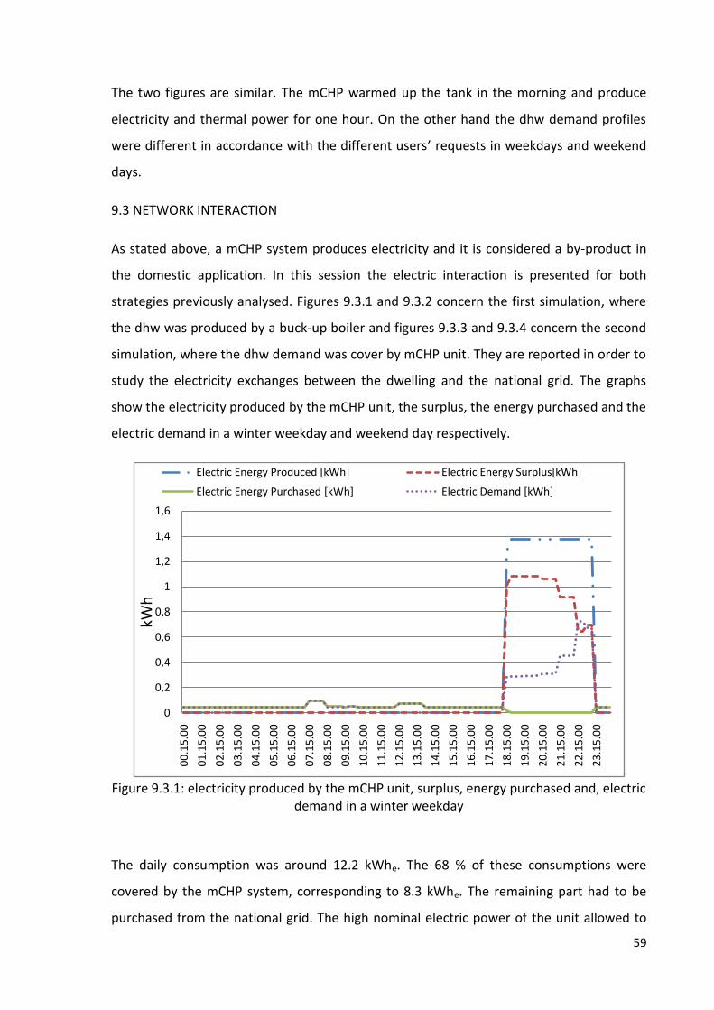
59

The two figures are similar. The mCHP warmed up the tank in the morning and produce

electricity and thermal power for one hour. On the other hand the dhw demand profiles

were different in accordance with the different users’ requests in weekdays and weekend

days.

9.3 NETWORK INTERACTION

As stated above, a mCHP system produces electricity and it is considered a by-product in

the domestic application. In this session the electric interaction is presented for both

strategies previously analysed. Figures 9.3.1 and 9.3.2 concern the first simulation, where

the dhw was produced by a buck-up boiler and figures 9.3.3 and 9.3.4 concern the second

simulation, where the dhw demand was cover by mCHP unit. They are reported in order to

study the electricity exchanges between the dwelling and the national grid. The graphs

show the electricity produced by the mCHP unit, the surplus, the energy purchased and the

electric demand in a winter weekday and weekend day respectively.

Figure 9.3.1: electricity produced by the mCHP unit, surplus, energy purchased and, electric

demand in a winter weekday

The daily consumption was around 12.2 kWhe. The 68 % of these consumptions were

covered by the mCHP system, corresponding to 8.3 kWhe. The remaining part had to be

purchased from the national grid. The high nominal electric power of the unit allowed to

0

0,2

0,4

0,6

0,8

1

1,2

1,4

1,6

00

.15

.00

01

.15

.00

02

.15

.00

03

.15

.00

04

.15

.00

05

.15

.00

06

.15

.00

07

.15

.00

08

.15

.00

09

.15

.00

10

.15

.00

11

.15

.00

12

.15

.00

13

.15

.00

14

.15

.00

15

.15

.00

16

.15

.00

17

.15

.00

18

.15

.00

19

.15

.00

20

.15

.00

21

.15

.00

22

.15

.00

23

.15

.00

kWh

Electric Energy Produced [kWh] Electric Energy Surplus[kWh]

Electric Energy Purchased [kWh] Electric Demand [kWh]

60

generate around 27.4 kWhe, of which 19.2 kWhe fed the grid. If all the electricity generated

was on site utilised, the system would provide to cover the total electrical demand and the

surplus would be around 15.2 kWhe.

Figure 9.3.2: electricity produced by the mCHP unit, surplus, energy purchased and electric

demand in a winter weekend day

The energy purchased profile and electric demand profile were overlapping until the mCHP

was turned off. In this case the simulation was different. The total electric demand was

11.71 kWh and only the 50 % was supply by the co generation unit. The difference

between this value and the value of the weekday simulation was due to the different

electricity demand profile. Therefore the majority of the electricity produced was sold

(around 21.5 kWhe that is 78 %).

Regarding the split model, where the mCHP warmed up the water tank in the morning and

operated for one hour, the underlying graphs are taken into account.

0

0,2

0,4

0,6

0,8

1

1,2

1,4

1,6

00

.15

.00

01

.15

.00

02

.15

.00

03

.15

.00

04

.15

.00

05

.15

.00

06

.15

.00

07

.15

.00

08

.15

.00

09

.15

.00

10

.15

.00

11

.15

.00

12

.15

.00

13

.15

.00

14

.15

.00

15

.15

.00

16

.15

.00

17

.15

.00

18

.15

.00

19

.15

.00

20

.15

.00

21

.15

.00

22

.15

.00

23

.15

.00

kWh



61

Figure 9.3.3: electricity produced by the mCHP unit under split pattern, surplus, energy purchased and electric demand in a winter weekday

The energy produced was 32.9 kWhe. It means an increase around 5.5 kWhe every day,

therefore an increase of 20 %. The daily consumption increased because the mCHP system

requested electricity to operate. The 73 % of the consumptions was covered by the mCHP

system, and the 27 % was imported. As state above the electricity produced by the unit

increased of 20 % and the electricity bought decreased only around 5 %. This is due to the

electric demand, which was low during the morning.


purchased and electric demand in a winter weekend day

0

0,2

0,4

0,6

0,8

1

1,2

1,4

1,6

00

.15

.00

01

.15

.00

02

.15

.00

03

.15

.00

04

.15

.00

05

.15

.00

06

.15

.00

07

.15

.00

08

.15

.00

09

.15

.00

10

.15

.00

11

.15

.00

12

.15

.00

13

.15

.00

14

.15

.00

15

.15

.00

16

.15

.00

17

.15

.00

18

.15

.00

19

.15

.00

20

.15

.00

21

.15

.00

22

.15

.00

23

.15

.00

kWh



0

0,2

0,4

0,6

0,8

1

1,2

1,4

1,6

00

.15

.00

01

.15

.00

02

.15

.00

03

.15

.00

04

.15

.00

05

.15

.00

06

.15

.00

07

.15

.00

08

.15

.00

09

.15

.00

10

.15

.00

11

.15

.00

12

.15

.00

13

.15

.00

14

.15

.00

15

.15

.00

16

.15

.00

17

.15

.00

18

.15

.00

19

.15

.00

20

.15

.00

21

.15

.00

22

.15

.00

23

.15

.00

kWh



62

The mCHP unit covered the 58 % of the demand. Thus there was a little increase respect to

the simulation with the back-up boiler.

Regarding the annual simulation is interesting to show the amount of the energy produced

that was sold. The underlying figure illustrates the annual percentage of the surplus for the

two scenarios reported above.

Figure 9.3.5: annual export proportion for mCHP plus boiler for DHW

Figure 9.3.6: annual export proportion for mCHP with split generation strategy

0

0,1

0,2

0,3

0,4

0,5

0,6

0,7

0,8

0,9

Export proportion

0

0,1

0,2

0,3

0,4

0,5

0,6

0,7

0,8

0,9

Export proportion

63

The maximum percentage value was around 77 % during the winter. Obviously in the first

case during the summer the value was equal to zero. On the other hand the minimum

value occurred in the summer in split generation strategy, when no space heating demand

was required, was around 62 %. Analysing this two values it is possible to note that the

system was oversized regarding the electric power. But the electricity is considering a by-

product and the capacity was chosen to cover the thermal demand.

64

10 MODELLING OF THE HOUSE WITH STIRLIG ENGINE

10.1 STIRLING ENGINE PLUS AUXILIARY BOILER WITH GAS FIRED BOILER FOR DHW

A new solution was modelled to meet the thermal demand of the dwelling. The circuit is

the same described for the ICE plus boiler and it is reported in APPENDIX III.

The internal combustion engine was replaced by a Stirling engine. The unit used was

manufactured by Inspirit, an English company. The Inspirit mCHP appliance had an rated

electric power output of 3 kW and rated thermal to electrical power ratio of 5. Therefore

this mCHP system, compared to the SenerTec ICE, presented a less electric capacity and a

greater thermal capacity. The Stirling engine had an electric efficiency of 16 % and a

thermal efficiency of 76 %, offering an overall efficiency around 92 %. These values, used in

the simulation, are given by the manufacturers [48]. The appliance could not operate alone

to achieve the required temperature of 21 °C. For this reason the unit was coupled with an

auxiliary boiler, as made previously. The boiler had a capacity of 20 kW and an efficiency of

85 %. Moreover a gas fired boiler was predicted to cover the dhw demand. The operation

assumed was always the same used in the ICE pattern both for space heating and dhw

requests. The Inspirit mCHP appliance was connected to the national grid and it fed the

grid when the electricity produced was greater than the demand. 1.58 1/h air changing was

used.

The figure 10.1.1 and 10.2.2 represent the gas consumption due to space heating,

composed of mCHP gas consumption and boiler gas consumption. Moreover the thermal

power produced by the two devices is reported. The graphs illustrate the profiles for a

typical cold weekday.

65


winter weekday

This figure is similar to figure 9.1.1. The boiler thermal output was equal. Indeed the boiler

worked continuously at 5 kWhth. The Inspirit mCHP appliance presented a thermal output

slightly higher than the SenerTec mCHP unit, but the ICE studied achieved its peak value

before. This was due to the different warm up delay time in accordance with [13].

Regarding the gas consumption the peak value of the previous device was greater than the

Stirling engine value. The difference was around 8 %. The operation characteristics of the

two heating systems were different during a warm day, as shown in the figure 10.1.2.

0

1

2

3

4

5

6

7

8

00

.15

.00

01

.15

.00

02

.15

.00

03

.15

.00

04

.15

.00

05

.15

.00

06

.15

.00

07

.15

.00

08

.15

.00

09

.15

.00

10

.15

.00

11

.15

.00

12

.15

.00

13

.15

.00

14

.15

.00

15

.15

.00

16

.15

.00

17

.15

.00

18

.15

.00

19

.15

.00

20

.15

.00

21

.15

.00

22

.15

.00

23

.15

.00

kWh



66


warm weekday

The mCHP system was able to cover the space heating demand almost alone, as

demonstrated for the ICE system. However in this case the operating characteristic was

different. The Inspirit mCHP appliance worked for a long period, then it was cut off and

then it returned to operate with a thermal peak lower than the rated thermal power

output. On the contrary in the previous case the ICE operated always at maximum thermal

output.

Working together the boiler and the mCHP unit were able to reach the set-point

temperature inside the zone during a winter day. The figure 10.1.2 shows the temperature

profile inside the four active zones.

0

0,5

1

1,5

2

2,5

3

3,5

4

4,5

5

00

.15

.00

01

.15

.00

02

.15

.00

03

.15

.00

04

.15

.00

05

.15

.00

06

.15

.00

07

.15

.00

08

.15

.00

09

.15

.00

10

.15

.00

11

.15

.00

12

.15

.00

13

.15

.00

14

.15

.00

15

.15

.00

16

.15

.00

17

.15

.00

18

.15

.00

19

.15

.00

20

.15

.00

21

.15

.00

22

.15

.00

23

.15

.00

kWh



67


weekday

As it is possible to note, the maximum temperature was 21 °C. If the Stirling system

operated alone, the temperature reached would be lower as figure 10.1.3 shows.


without boiler

0

5

10

15

20

25

0

5

10

15

20

25

00

.15

.00

01

.15

.00

02

.15

.00

03

.15

.00

04

.15

.00

05

.15

.00

06

.15

.00

07

.15

.00

08

.15

.00

09

.15

.00

10

.15

.00

11

.15

.00

12

.15

.00

13

.15

.00

14

.15

.00

15

.15

.00

16

.15

.00

17

.15

.00

18

.15

.00

19

.15

.00

20

.15

.00

21

.15

.00

22

.15

.00

23

.15

.00

kW

tem

per

atu

re [

°C]



Boiler Heating Output Rate [kW] mCHP Thermal Power Produced [kW]

0

2

4

6

8

10

12

14

16

0

2

4

6

8

10

12

14

00

.15

…

01

.15

…

02

.15

…

03

.15

…

04

.15

…

05

.15

…

06

.15

…

07

.15

…

08

.15

…

09

.15

…

10

.15

…

11

.15

…

12

.15

…

13

.15

…

14

.15

…

15

.15

…

16

.15

…

17

.15

…

18

.15

…

19

.15

…

20

.15

…

21

.15

…

22

.15

…

23

.15

…

kW

tem

per

atu

re [

°C]



mCHP Thermal Power Produced [kW]

68

The maximum temperature achieved was slightly higher than 13 °C. The kitchen

temperature profile presents in figure 10.1.2 and 10.1.3 two peak in the morning and

during the lunch time due to the cookers usage.

10.2 STIRLING ENGINE PLUS AUXILIARY BOILER SPLIT GENERATION STRATEGY

This simulation was carried out under split generation strategy. The Inspirit mCHP

appliance supplied both central heating and dhw demands. APPENDIX IV gives an outline of

the curcuit.

The unit operated 60 minutes in the morning to heat a water tank. The water tank capacity

was 420 litres in order to maintain the temperature inside the tank over than 45 °C. The

figure 10.2.1 describes the operation characteristics of the mCHP and boiler and the dhw

profiles in a winter weekday.


winter weekday

The following figure shows as the temperature inside the tank was over 45 °C during the

day, as required. Moreover the graph presents the dhw consumption in litres.

0

1

2

3

4

5

6

7

8

00

.15

.00

01

.15

.00

02

.15

.00

03

.15

.00

04

.15

.00

05

.15

.00

06

.15

.00

07

.15

.00

08

.15

.00

09

.15

.00

10

.15

.00

11

.15

.00

12

.15

.00

13

.15

.00

14

.15

.00

15

.15

.00

16

.15

.00

17

.15

.00

18

.15

.00

19

.15

.00

20

.15

.00

21

.15

.00

22

.15

.00

23

.15

.00

kWh



DHW demand [kWh]

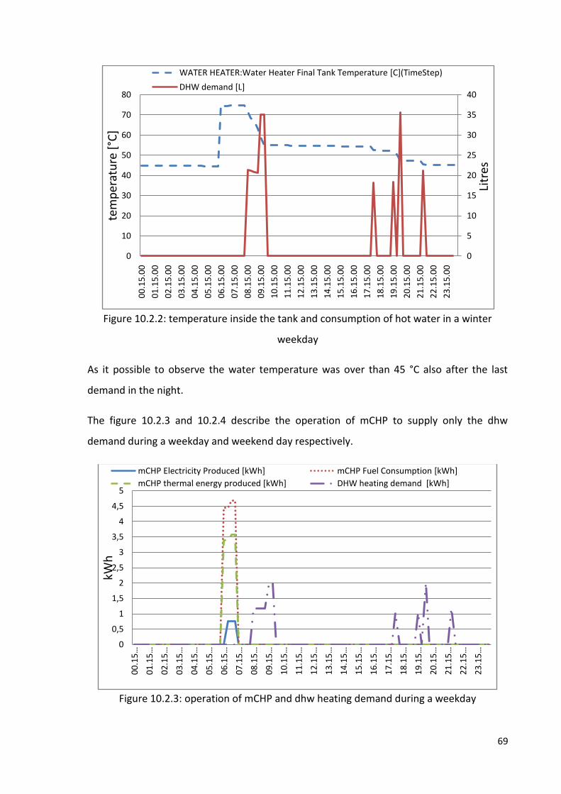
69


weekday

As it possible to observe the water temperature was over than 45 °C also after the last

demand in the night.

The figure 10.2.3 and 10.2.4 describe the operation of mCHP to supply only the dhw

demand during a weekday and weekend day respectively.

Figure 10.2.3: operation of mCHP and dhw heating demand during a weekday

0

5

10

15

20

25

30

35

40

0

10

20

30

40

50

60

70

80

00

.15

.00

01

.15

.00

02

.15

.00

03

.15

.00

04

.15

.00

05

.15

.00

06

.15

.00

07

.15

.00

08

.15

.00

09

.15

.00

10

.15

.00

11

.15

.00

12

.15

.00

13

.15

.00

14

.15

.00

15

.15

.00

16

.15

.00

17

.15

.00

18

.15

.00

19

.15

.00

20

.15

.00

21

.15

.00

22

.15

.00

23

.15

.00

Litr

es

tem

per

atu

re [

°C]

WATER HEATER:Water Heater Final Tank Temperature [C](TimeStep)

DHW demand [L]

0

0,5

1

1,5

2

2,5

3

3,5

4

4,5

5

00

.15

…

01

.15

…

02

.15

…

03

.15

…

04

.15

…

05

.15

…

06

.15

…

07

.15

…

08

.15

…

09

.15

…

10

.15

…

11

.15

…

12

.15

…

13

.15

…

14

.15

…

15

.15

…

16

.15

…

17

.15

…

18

.15

…

19

.15

…

20

.15

…

21

.15

…

22

.15

…

23

.15

…

kWh



70

Figure 10.2.4: operation of mCHP and dhw heating demand during weekend day

The unit operated continuously for one hour to heat the water tank. Obviously the

operation characteristic and the gas consumption were both for weekday and weekend

day the same. The dhw profiles changed because of different hot water usages. In this case

the electricity produced in the morning was lower than the electricity produced by the

SenerTec mCHP appliance due to the different rated electric power output (3 kWhe against

5.5 KWhe).

10.3 NETWORK INTERACTION

As done above for SenerTec mCHP appliance, the network interaction is presented for both

strategies analysed. Figures 10.3.1 and 10.3.2 concern the first simulation, where the dhw

was produced by a buck-up boiler and figures 9.3.3 and 9.3.4 concern the second

simulation, where the dhw demand was cover by mCHP unit. The graphs show the

electricity produced by the mCHP system, the surplus, the energy purchased and the

electric demand in a winter weekday and weekend day respectively.

0

0,5

1

1,5

2

2,5

3

3,5

4

4,5

5

00

.15

.…

01

.15

.…

02

.15

.…

03

.15

.…

04

.15

.…

05

.15

.…

06

.15

.…

07

.15

.…

08

.15

.…

09

.15

.…

10

.15

.…

11

.15

.…

12

.15

.…

13

.15

.…

14

.15

.…

15

.15

.…

16

.15

.…

17

.15

.…

18

.15

.…

19

.15

.…

20

.15

.…

21

.15

.…

22

.15

.…

23

.15

.…

kWh



71

Figure 10.3.1: electricity produced by the mCHP unit, surplus, energy purchased and,

electric demand in a winter weekday

The electricity purchased profile and electric demand were overlapping when the mCHP

did not operate. The Inspirit mCHP appliance covered the 65 % of the electricity demand.

This value was similar to the SenerTec unit coverage. The most important difference

between the two systems was the energy surplus. In this case only 6.2 kWhe were sold,

corresponding to 44 % of the total electricity produced. This was due to the nominal

electric power, which was much lower than the SenerTec nominal electric power. If all the

electricity generated was on site utilised, the system would provide to cover the total

electrical demand.

0

0,1

0,2

0,3

0,4

0,5

0,6

0,7

0,8

00

.15

.…

01

.15

.…

02

.15

.…

03

.15

.…

04

.15

.…

05

.15

.…

06

.15

.…

07

.15

.…

08

.15

.…

09

.15

.…

10

.15

.…

11

.15

.…

12

.15

.…

13

.15

.…

14

.15

.…

15

.15

.…

16

.15

.…

17

.15

.…

18

.15

.…

19

.15

.…

20

.15

.…

21

.15

.…

22

.15

.…

23

.15

.…

kWh



0

0,1

0,2

0,3

0,4

0,5

0,6

0,7

0,8

00

.15

.00

01

.15

.00

02

.15

.00

03

.15

.00

04

.15

.00

05

.15

.00

06

.15

.00

07

.15

.00

08

.15

.00

09

.15

.00

10

.15

.00

11

.15

.00

12

.15

.00

13

.15

.00

14

.15

.00

15

.15

.00

16

.15

.00

17

.15

.00

18

.15

.00

19

.15

.00

20

.15

.00

21

.15

.00

22

.15

.00

23

.15

.00

kWh



72

Figure 10.3.2: electricity produced by the mCHP unit, surplus, energy purchased and electric demand in a winter weekend day

The 50 % of the electricity consumed had to be purchase. The remaining part was produce

by the co generator unit. Indeed the demand increased in the afternoon when the unit was

off. Therefore the electric surplus raised and the 59 % of the electricity produced fed the

national grid.

Taking into account the split model, where the mCHP warmed up the water tank in the

morning and operated for one hour, the following graphs illustrate the network

interaction.


purchased and electric demand in a winter weekday

The electricity produced was 16.3 kWh. The 67 % of the electric demand was supplied by

the mCHP and the 57 % of the energy produced was on site utilized. The electricity

production increased by 2.21 kWhe, corresponding to an increase of 16 % compared to the

previous production.

0

0,1

0,2

0,3

0,4

0,5

0,6

0,7

0,8

00

.15

.00

01

.15

.00

02

.15

.00

03

.15

.00

04

.15

.00

05

.15

.00

06

.15

.00

07

.15

.00

08

.15

.00

09

.15

.00

10

.15

.00

11

.15

.00

12

.15

.00

13

.15

.00

14

.15

.00

15

.15

.00

16

.15

.00

17

.15

.00

18

.15

.00

19

.15

.00

20

.15

.00

21

.15

.00

22

.15

.00

23

.15

.00

kWh



73


purchased and electric demand in a winter weekend day

In this case the system covered the 54 % of the consumption, corresponding to 7.3 kWhe,

while 6.2 kWhe was purchased.

Also for Stirling simulation the annual amount of the energy produced that was sold is

presented. This profile is represented in the following figure.

Figure 10.3.5: annual export proportion for mCHP plus boiler for DHW

0

0,1

0,2

0,3

0,4

0,5

0,6

0,7

0,8

00

.15

.00

01

.15

.00

02

.15

.00

03

.15

.00

04

.15

.00

05

.15

.00

06

.15

.00

07

.15

.00

08

.15

.00

09

.15

.00

10

.15

.00

11

.15

.00

12

.15

.00

13

.15

.00

14

.15

.00

15

.15

.00

16

.15

.00

17

.15

.00

18

.15

.00

19

.15

.00

20

.15

.00

21

.15

.00

22

.15

.00

23

.15

.00

kWh



0

0,1

0,2

0,3

0,4

0,5

0,6

Export proportion

74

Figure 10.3.6: annual export proportion for mCHP with split generation strategy

As noted for the ICE system, the peak value of the electricity exported was during the

winter and it amounted to 56 %. The percentage was lower than the same value noted for

the SenerTec mCHP appliance. The minimum percentage, which was equal to 10 %, was

much less than the previous simulation. This was due to the different electric capacity.

Indeed the Inspirit mchp appliance presented a nominal power lower than the SenerTec

unit.

0

0,1

0,2

0,3

0,4

0,5

0,6

0,7

Export proportion

75

11 ANNUAL SUMMARY

Three different solutions were compared in order to demonstrate the possible savings:

1. Boiler with a thermal capacity of 40 kW (reference scenario);

2. The SenerTec mCHP appliance with a rated electric power output of 5.5 plus a

boiler with a thermal capacity of 20 kW;

3. The Inspirit mCHP appliance with a rated electric power output of 3 kW plus a boiler

with a thermal capacity of 20 kW;

An environmental and economical analysis was carried out between these three systems.

It is worth taking into account the model considering an extra electricity consumption due

to the electric parasitic load of the boiler. It was made to compare the economic and

environmental savings with the principal simulation, where the extra consumption was

neglected. The annual electricity consumption was around 880 kWh for the boiler in the

reference scenario. Regarding the co generation scenario the auxiliary boiler coupled with

SenerTec mCHP appliance presented parasitic electric load around 595 kWh and the

Inspirit mCHP appliance had 580 kWh.

11.1 ECONOMIC PERFORMANCE

The economic performances analysis was based on the electricity price of 0.10108 €/kWh

with electricity annual consumption ranged from 2641 kWhe to 4440 kWhe. In this case

only the energy price was considered, all taxes excluded. On the other hand all taxes

included price for this range of electricity consumed was 0.248930 €/kWh. If the

consumption overtakes 4440 kWhe/y the all taxes included price and all taxes excluded

price are respectively of 0.295690 €/kWh and 0.10571 €/kWh. All the prices utilized are in

accordance to [46]. An hypothetical feed-in-tariff was modelled. It was supposed to have

three different selling prices corresponding to 50 %, 75 % and 100 % of the purchase price.

76

11.1.1 Analysis without parasitic electric load and all taxes excluded price

Tables 11.1.1.1, 11.1.1.2 and 11.1.1.3 illustrate the annual economic performances of the

different scenarios considered with a feed-in-tariff of 50 %, 75 % and 100 % of the

purchase price.

Configuration Gas

Consumption

[€]

Electricity

Consumption

[€]

Income

From

Electricity

[€] 50%

Net

Annual

Expences

[€] 50%

Savings

[%]

BOILER&Gas

heater WT (95L)

1192.66 379.83 1572.49

SENERTECH&Gas

heater WT (95L)

1411.21 279.93 156.83 1534.32 2.43

INSPIRIT&Gas

heater WT (95L)

1347.75 290.01 53.64 1584.13 -0.74

SENERTECH

separate hours

(420L)

1474.36 272.92 228.59 1518.70 3.42

INSPIRIT

separate hours

(420L)

1372.12 284.61 66.92 1589.81 -1.10

Table 11.1.1.1: annual economic performance for all scenarios with feed-in-tariff of 50 % of the purchase price

The Inspirit mCHP appliance had no economic benefits due to the low electricity sold. The

expense in split generation scenario increased if compared to Inspirit and gas heater

because of increased the gas consumption. The gas expense increased more than the

income from electricity. On the other hand for the SenerTec mCHP appliance the split

generation had more savings than the SenerTec and gas heater.

77

Configuration Gas

Consumption

[€]

Electricity

Consumption

[€]

Income

From

Electricity

[€] 75%

Net

Annual

Expences

[€] 75%

Savings

[%] 75%

BOILER&Gas

heater WT (95L)

1192.66 379.83 1572.49

SENERTECH&Gas

heater WT (95L)

1411.21 279.93 235.25 1455.90 7.41

INSPIRIT&Gas

heater WT (95L)

1347.75 290.01 80.46 1557.31 0.97

SENERTECH

separate hours

(420L)

1474.36 272.92 342.88 1404.41 10.69

INSPIRIT

separate hours

(420L)

1372.12 284.61 100.38 1556.35 1.03


Configuration Gas

Consumption

[€]

Electricity

Consumption

[€]

Income

From

Electricity

[€] 100%

Net

Annual

Expences

[€] 100%

Savings

[%] 100%

BOILER&Gas

heater WT (95L)

1192.66 379.83 1572.49

SENERTECH&Gas

heater WT (95L)

1411.21 279.93 313.66 1377.49 12.40

INSPIRIT&Gas

heater WT (95L)

1347.75 290.01 107.28 1530.49 2.67

SENERTECH

separate hours

(420L)

1474.36 272.92 457.17 1290.11 17.96

INSPIRIT separate

hours (420L)

1372.12 284.61 133.84 1522.89 3.15


Both simulations (feed-in-tariff of 75 % of the purchase price and feed-in-tariff of 100 % of

the purchase price) demonstrated that the savings in split generation were more than the

savings in the simple mCHP scenario due to the electricity sold during the morning, when

the mCHP system warmed up the water tank. The SenerTec mCHP appliance with split

generation had always the higher economic benefits.

78

11.1.2 Savings with parasitic electric load and all taxes excluded price

The follow table describes economic savings if parasitic electric load was considered.

Configuration Savings [%]

(feed-in-tariff

50%)

Savings [%]

(feed-in-tariff

75%)

Savings [%]

100% (feed-in-

tariff)

BOILER&Gas

heater WT (95L)

/ / /

SENERTECH&Gas

heater WT (95L)

7.15 10.92 14.69

INSPIRIT&Gas

heater WT (95L)

3.71 4.61 5.51

SENERTECH

separate hours

(420L)

9.41 16.02 22.63

INSPIRIT separate

hours (420L)

5.01 6.80 8.58

Table 11.1.2.1: annual economic savings for all scenarios taking into account the parasitic electric load

Obviously taking into account the extra electricity consumption of the boiler the economic savings increased in every scenario.

11.1.3 Analysis without parasitic electric load and all taxes included price

Tables 11.1.3.1, 11.1.3.2 and 11.1.3.3 summarize the results.

Configuration Gas

Consumption

[€]

Electricity

Consumption

[€]

Income

From

Electricity

[€] 50%

Net

Annual

Expences

[€] 50%

Savings

[%] 50%

BOILER&Gas

heater WT (95L)

1192.66 935.40 2128.07

SENERTECH&Gas

heater WT (95L)

1411.21 689.39 386.23 1714.38 19.44

INSPIRIT&Gas

heater WT (95L)

1347.75 714.21 132.09 1929.87 9.31

SENERTECH

separate hours

(420L)

1474.36 672.13 562.94 1583.55 25.59

INSPIRIT

separate hours

(420L)

1372.12 700.91 164.81 1908.23 10.33


79

Configuration Gas

Consumption

[€]

Electricity

Consumption

[€]

Income

From

Electricity

[€] 75%

Net

Annual

Expences

[€] 75%

Savings

[%] 75%

BOILER&Gas

heater WT (95L)

1192.66 935.40 2128.07

SENERTECH&Gas

heater WT (95L)

1411.21 689.39 579.34 1521.27 28.51

INSPIRIT&Gas

heater WT (95L)

1347.75 714.21 198.14 1863.82 12.42

SENERTECH

separate hours

(420L)

1474.36 672.13 844.41 1302.08 38.81

INSPIRIT

separate hours

(420L)

1372.12483 700.91 247.21 1825.82 14.20


Configuration Gas Consumption [€]

Electricity Consumption [€]

Income From Electricity [€] 100%

Net Annual Expences [€] 100%

Savings [%] 100%

BOILER&Gas heater WT (95L)

1192.66 935.40 2128.07

SENERTECH&Gas heater WT (95L)

1411.21 689.39 772.45 1328.15 37.59

INSPIRIT&Gas heater WT (95L)

1347.75 714.21 264.19 1797.77 15.52

SENERTECH separate hours (420L)

1474.36 672.13 1125.88 1020.62 52.04

INSPIRIT separate hours (420L)

1372.12 700.91 329.61 1743.42 18.07


In every scenario there were economic benefits. These benefits increased if compared to

the simulation with all taxes excluded price due to the feed-in-tariff rise. The Inspirit mCHP

appliance economic savings were always positive, but they were much lower than the

SenerTec benefits.

80

11.1.4 Savings with parasitic electric load and all taxes included price

The follow table shows economic savings taking into account parasitic electric load.


(feed-in-tariff

50%)

Savings [%] (feed-

in-tariff 75%)

Savings [%] 100%

(feed-in-tariff)

BOILER&Gas heater

WT (95L)

/ / /

SENERTECH&Gas

heater WT (95L)

30.40 36.49 42.57

INSPIRIT&Gas heater

WT (95L)

21.29 22.74 24.18

SENERTECH separate

hours (420L)

37.72 48.38 59.05

INSPIRIT separate

hours (420L)

24.93 27.81 30.70

Table 11.1.4.1: annual economic savings for all scenarios taking into account the parasitic electric load

Also in this case, if extra electricity consumption was considered, the benefits increased.

The high value predicted for the SenerTec mCHP appliance was due to the increase of sold

electricity. Indeed the electricity produced during the morning was produced when the

electric demand was low.

11.2 CARBON SAVINGS

To evaluate the carbon savings it is necessary to have the emission factors. It is possible to

find in literature the follow values for the Italian situation:

0.53 kg CO2/kWh for electricity [11];

0.19 CO2/kWh for burned natural gas [32];

The underlying table reports the annual carbon savings predicted for all scenarios if no

extra electricity consumption was considered.

81

Configuration Carbon Emission

From Gas [kg]

Carbon Emission

From El [kg]

Total

[kg]

Savings

[kg]

Savings

[%]

BOILER&Gas heater

WT (95L)

5387.19 1991.58 7378.77

SENERTECH&Gas

heater WT (95L)

6374.38 1467.80 7842.18 -463.40 -6.28

INSPIRIT&Gas heater

WT (95L)

6087.73 1520.63 7608.36 233.81 -3.11

SENERTECH separate

hours (420L)

6659.61 1431.04 8090.66 -482.29 -9.65

INSPIRIT separate

hours (420L)

6197.81 1492.31 7690.12 400.53 -4.22

Table 11.2.1: annual carbon emissions predicted for all scenarios without parasitic electric

load

If the parasitic electric load of the boiler was not applied, no savings was predicted. The

worst scenario was the SENERTECH separate hours, where the gas consumption increased

if compared to SENERTECH&Gas heater WT. The ICE heating systems presented in every

scenario a total carbon emission greater than the Stirling systems. It is possible to observe

also if parasitic electric load of the boiler was considered, as the follow table reported.


BOILER&Gas heater WT (95L) /

SENERTECH&Gas heater WT (95L) 0.14

INSPIRIT&Gas heater WT (95L) 2.16

SENERTECH separate hours (420L) -3.11

INSPIRIT separate hours (420L) 1.86

Table 11.2.2: annual carbon savings predicted for all scenarios with parasitic electric load

In this case carbon savings were achieved. Only SENERTECH separate hours scenario had

no environmental benefits due to the high gas consumption. The best performances were

achieved by the Stirling engine. In the INSPIRIT&Gas heater WT (95L) scenario the carbon

emission decreased around 2 % compared to the reference scenario.

82

12 CONCLUSIONS

In itially different types of mCHP systems were presented in order to have a general idea

regarding the different technologies. It was described the commercial available systems

and the current state of investigation, where the main prototypes were reported.

Subsequently a reference scenario was model and daily results reported and analysed.

Under two different configurations two unlike mCHP systems were studied in order to

compare the annual and daily characteristics. All the simulation was carried out using the

software Energy Plus. The underlying conclusions were achieved:

The optimal value regarding the air changing per hour was 1.58 1/h.

The mCHP systems were not able to cover the dwelling thermal demand and they

had to be couple with an auxiliary boiler. This was due to the high space heating

request if compared whit the rated thermal power output of the co generation

units installed.

Under the split generation strategy the size of the water tank was 420 L. In this

case the water inside the tank had a temperature over than 45 °C after the

demand event. This is important because the dhw can not have a lower

temperature.

Regarding the network interaction the two mCHP systems could cover the electric

demand if all the energy produced was on site utilized.

The ICE in split generation strategy had the best daily performance. It was able to

supply the 73 % of the electric consumption. This was due to the electric demand

profile. Indeed the majority of the domestic requests occurred during the mCHP

operation.

The annual analysis demonstrated that the SenerTec mCHP appliance operating

with split generation strategy had the maximum economic benefits. This was due

to the high rated electric power output if compared with the electric nominal

capacity of Inspirit appliance. On the other hand this unit presented no carbon

saving in both configurations (with and without parasitic electric load) because

the carbon emissions, due to the gas burned, increased more than the electric

consumption decrease.

83

All configurations achieved economic savings except the Inspirit mCHP appliance

if no extra electricity consumptions were considered.

Regarding the carbon savings the best scenario was the Inspirit mCHP appliance

with Gas heater water tank. The system achieved a carbon savings over than 2 %

if compared with the reference scenario.

The SenerTec unit had gas consumptions always more than the Inspirit systems.

It was noted as more power is installed, more economic savings are achieved, in

accordance with [33].

84

13 REFERENCE

1. Nelson Fumo, Pedro J. Mago, Louay M. Chamra; Analysis of cooling, heating, and power

systems based on site energy consumption. Applied Energy 86 (2009) 928–932.

2. Kari Alanne, Arto Saari; Sustainable small-scale CHP technologies for buildings: the basis

for multi-perspective decision-making. Renewable and Sustainable Energy Reviews 8

(2004) 401–431.

3. Mark Hinnells; Combined heat and power in industry and buildings. Energy Policy 36

(2008) 4522–4526.

4. M. Dentice d’ Accadia, M. Sasso, S. Sibilio, L. Vanoli; Micro-combined heat and power in

residential and light commercial applications. Applied Thermal Engineering 23 (2003)

1247-1259.

5. Asmus P. The war against terrorism helps build the case for distributed renewables. The

Electricity Journal 2001; December:75–80.

6. R. Possidente, C. Roselli, M. Sasso, S. Sibilio; Experimental analysis of micro-

cogeneration units based on reciprocating internal combustion engine. Energy and

Buildings 38 (2006) 1417–1422.

7. Michele Bianchi, Pier Ruggero Spina; Integrazione di sistemi cogenerativi innovativi di

piccolissima taglia nelle reti di distribuzione dell’energia elettrica, termica e frigorifera.

Report RdS/2010/220 p. 1-112.

8. M. Bianchi P. R. Spina G. Tomassetti, D. Forni E. Ferrero; Le tecnologie innovative ed

efficienti nei sistemi di generazione in assetto co-trigenerativo e nei sistemi integrati

con unità a pompa di calore nelle applicazioni industriali e del terziario. Report

RSE/2009/18 p.1-187.

9. Bernd Thomas; Benchmark testing of Micro-CHP units. Applied Thermal Engineering 28

(2008) 2049–2054.

10. Enrico Saverio Barbieri, Pier Ruggero Spina, Mauro Venturini; Analysis of innovative

micro-CHP systems to meet household energy demands. Applied Energy 97 (2012) 723–

733

11. Carlo Roselli, Maurizio Sasso, Sergio Sibilio, Peter Tzscheutschler; Experimental analysis

of microcogenerators based on different prime movers. Energy and Buildings 43 (2011)

796–804.

85

12. H. Leibowitz; Cost of effective small scale ORC systems for power recovery from low

grade heat sources. 2006 ASME International Mechanical Engineering Congress and

Exposition November 5-10, 2006, Chicago, Illinois, USA.

13. Jeremy Harrison; Micro Combined Heat & Power. EA Technology.

14. Jenn Jiang Hwang, Meng Lin Zou ;Development of a proton exchange membrane fuel

cell cogeneration system. Journal of Power Sources 195 (2010) 2579–2585.

15. A.D. Peacock and M. Newborough; Micro-Generation opportunities in the UK residential

sector. World Renewable Energy Congress VIII (WREC 2004).

16. Alessia Arteconi, Carlo Maria Bartolini and Caterina Brandoni; Energy and economic

analysis of small-scale distributed generation in the residential sector. 14th Stirling

Engines Conference, 2009.

17. M. Bell, M Swinton, E. Entchev, J. Gusdorf, W. Kalbfleisch, R. Marchand and F.

Szadkowski; Testing Residential Combined Heat and Power Systems at the Canadian

Center for Housing Technology.

18. Viktor Dorer, Andreas Weber; Energy and CO2 emissions performance assessment of

residential micro-cogeneration systems with dynamic whole-building simulation

programs. Energy Conversion and Management 50 (2009) 648–657.

19. A.D. Peacock and M. Newborough; Impact of micro-CHP systems on domestic sector

CO2 emissions. Applied Thermal Engineering 25 (2005) 2653–2676.

20. M Newborough; Assessing the benefits of implementing micro-CHP systems in the UK.

Proceedings of the Institution of Mechanical Engineers, Part A: Journal of Power and

Energy 2004 pag. 218-203.

21. A.D. Peacocka, M. Newborough; Effect of heat-saving measures on the CO2 savings

attributable to micro-combined heat and power (mCHP) systems in UK dwellings.

Energy 33 (2008) pag. 601–612.

22. Kris R. Voorspools and William D. D’haeseleerz; The evaluation of small cogeneration

for residential heating. International Journal of Energy Research 2002; 26: pag. 1175–

1190.

23. European Committee for Standardisation; Indoor environmental input parameters for

design and assessment of energy performance of buildings addressing indoor air

quality, thermal environment, lighting and acoustics. CEN/TC 156.

86

24. Ministero dello sviluppo economico; Integrazioni al decreto legislativo 8 febbraio 2007,

n. 20, di attuazione della direttiva 2004/8/CE sulla promozione della cogenerazione

basata su una domanda di calore utile sul mercato interno dell’energia, e modifi cativa

della direttiva 92/42/CE. DECRETO 4 August 2011.

25. Bancha Kongtragool, Somchai Wongwises; Thermodynamic Analysis of a Stirling engine

including dead volumes of hot space, cold space and regenerator. Renewable Energy 31

(2006) 345–359.

26. Autorità per l’Energia Elettrica e il Gas; Testo integrato delle modalità e delle condizioni

tecnico-economiche per lo scambio sul posto (TISP. Deliberazione 3 giugno 2008 -

ARG/elt 74/08).

27. M.A. Ehyaei, A. Mozafari; Energy, economic and environmental (3E) analysis of a micro

gas turbine employed for on-site combined heat and power production. Energy

Buildings (2009), doi:10.1016/j.enbuild.2009.09.001.

28. T.J. Hammons; Impact of electric power generation on green house gas emissions in

Europe: Russia, Greece, Italy and views of the EU Power Plant Supply Industry – a critical

analysis. Electrical Power and Energy Systems 28 (2006) 548–564.

29. Franco Di Andrea, Andrea Danese; Misure dei consumi di energia elettrica nel settore

domestico Risultati delle campagne di rilevamento dei consumi elettrici presso 110

abitazioni in Italia. Politecnico di Milano (2004).

30. Michele De Carli; Indoor Environmental Quality. Energy and Buildings Class 2012

University of Padue.

31. Samantha Graci; Sistemi per la preparazione dell’ACS. Heating and Cooling Plants Class

2012 University of Padue.

32. Georgios Gkounis; Experimental and theoretical analysis of the performance of micro

co-generation systems based in various technologies in UK dwellings. Second year PHD

annual progression Research Report, Northumbria University.

33. Carbon Trust, Micro-CHP Accelerator. Final Report 2011.

34. Tie Li, DaWei Tang, Zhigang Li, Jinglong Du, Tian Zhou, Yu Jia; Development and test of a

Stirling engine driven by waste gases for the micro-CHP system. Applied Thermal

Engineering 33-34 (2012) 119-123.

87

35. Jarosław Milewski, Łukasz Szabłowski, Jerzy Kuta; Control strategy for an Internal

Combustion engine fuelled by Natural Gas operating in Distributed Generation. Energy

Procedia 14 (2012) 1478-1483.

36. Energy Plus Documentation; Engineering Reference.

37. Rates of Electricity and Gas available at autorita.energia.it

38. http://www.microchap.info/rankine_engine.htm

39. Ellis MW; Fuel cells for building applications. USA: ASHRAE; 2002.

40. Industrial and commercial cogeneration. Chapter 4: Characterization of the

Technologies for Cogeneration. February 1983. p. 117–165.

41. http://www.microchap.info/stirling_engine.htm

42. http://www.microchap.info/other_technologies.htm

43. Ryan O’hayre, Suk-Won Cha, Whitney Colella, Fitz B.Prinz; Fuel Cell Fundamentals.

44. http://www.microchap.info/fuel_cell.htm

45. Commission of the European Communities. DEMAND-SIDE MANAGEMENT End-use

metering campaign in 400 households of the European Community Assessment of the

Potential Electricity Savings. January 2002.

46. http://www.autorita.energia.it/it/index.htm.

47. http://www.mtt-eu.com/applications/micro-chp.

48. http://www.inspiritenergy.com/producttechnology.html.

http://www.microchap.info/stirling_engine.htm

http://www.microchap.info/other_technologies.htm

http://www.microchap.info/fuel_cell.htm

http://www.mtt-eu.com/applications/micro-chp

http://www.inspiritenergy.com/producttechnology.html

88

APPENDIX I: DHW circuit

89

APPENDIX II: circuit space heating with boiler

90

APPENDIX III: circuit space heating with mCHP plus boiler

91

APPENDIX IV: circuit space heating with mCHP plus boiler in split generation strategy

1 introduction - universit degli studi di padova

Documents