1

Introduction to Introduction to Hypothesis Hypothesis TestingTesting

2

What is a Hypothesis?What is a Hypothesis? A hypothesis is a claim A hypothesis is a claim

(assumption) about a (assumption) about a

population parameter:population parameter:

population meanpopulation mean

population proportionpopulation proportion

Example: The mean monthly cell phone bill of this city is = $42

Example: The proportion of adults in this city with cell phones is p = .68

3

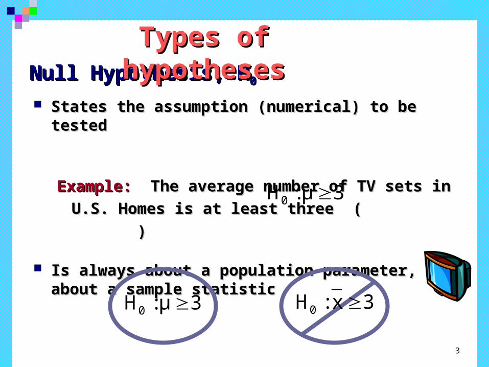
Null Hypothesis, HNull Hypothesis, H00

States the assumption (numerical) to be testedStates the assumption (numerical) to be tested

Example:Example: The average number of TV sets in U.S. The average number of TV sets in U.S.

Homes is at least three ( )Homes is at least three ( )

Is always about a population parameter, not about a Is always about a population parameter, not about a sample statistic sample statistic

3μ:H0

3μ:H0 3x:H0

Types of Types of hypotheseshypotheses

4

Begin with the assumption that the null hypothesis Begin with the assumption that the null hypothesis is trueis true Similar to the notion of innocent until proven Similar to the notion of innocent until proven

guiltyguilty May or may not be rejectedMay or may not be rejected

(continued)(continued)

Types of Types of hypotheseshypothesesNull Hypothesis, HNull Hypothesis, H00

5

Alternative Hypothesis, HAlternative Hypothesis, HAA

Is the opposite of the null hypothesisIs the opposite of the null hypothesis

e.g.: The average number of TV sets in U.S. e.g.: The average number of TV sets in U.S.

homes is less than 3 ( Hhomes is less than 3 ( HAA: : < 3 ) < 3 )

May or may not be acceptedMay or may not be accepted

Is generally the hypothesis that is believed (or Is generally the hypothesis that is believed (or

needs to be supported) by the researcherneeds to be supported) by the researcher

Types of Types of hypotheseshypotheses

Population

Claim: thepopulationmean age is 50.(Null Hypothesis:

REJECT

Supposethe samplemean age is 20: x = 20

SampleNull Hypothesis

20 likely if = 50?Is

Hypothesis Testing Hypothesis Testing ProcessProcess

If not likely,

Now select a Now select a random samplerandom sample

H0: = 50 )

x

7

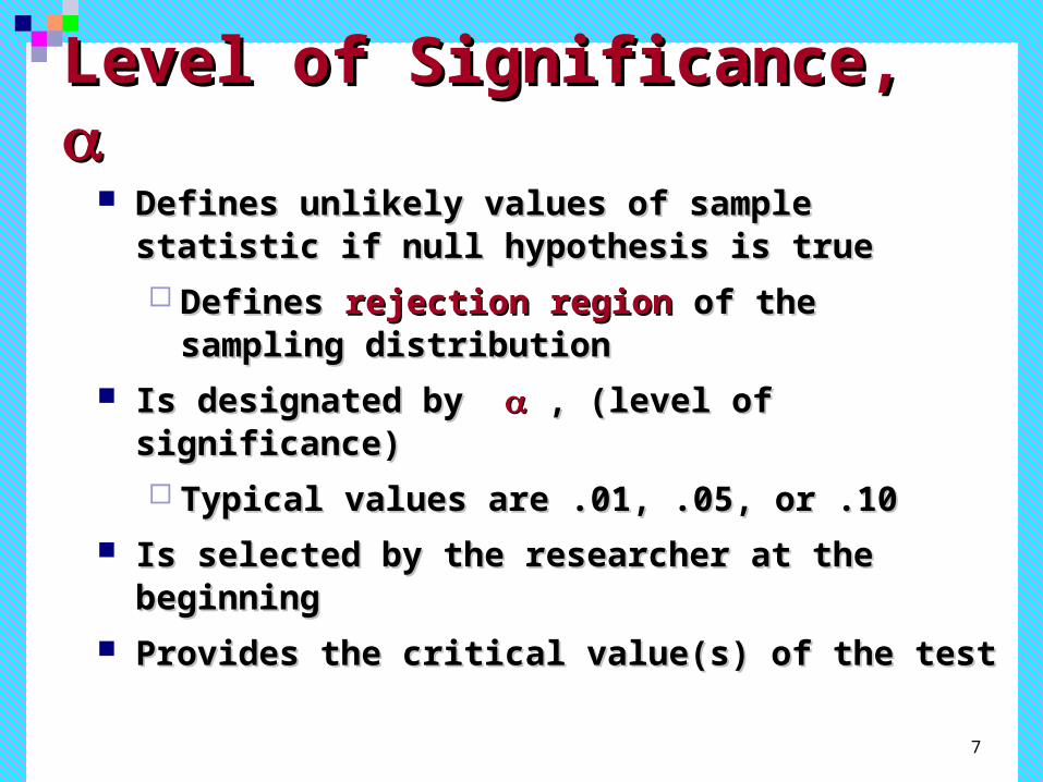
Level of Significance, Level of Significance, Defines unlikely values of sample statistic if null Defines unlikely values of sample statistic if null

hypothesis is truehypothesis is true

Defines Defines rejection regionrejection region of the sampling of the sampling distributiondistribution

Is designated by Is designated by , (level of significance) , (level of significance)

Typical values are .01, .05, or .10Typical values are .01, .05, or .10

Is selected by the researcher at the beginningIs selected by the researcher at the beginning

Provides the critical value(s) of the test Provides the critical value(s) of the test

8

Level of Significance and the Level of Significance and the Rejection RegionRejection Region

H0: μ ≥ 3

HA: μ < 3 0

H0: μ ≤ 3

HA: μ > 3

H0: μ = 3

HA: μ ≠ 3

/2

Represents critical value

Lower tail test

Level of significance = Level of significance =

0

0

/2

Upper tail test

Two tailed test

Rejection region is shaded

9

Reject HReject H00Do not reject HDo not reject H00

The cutoff value, , is The cutoff value, , is

called a called a critical valuecritical value

Lower Tail TestsLower Tail Tests

-z-zαα

xxαα

--zzαα

00

μμ

H0: μ ≥ 3

HA: μ < 3

n

σzμx

Types of testTypes of test

10

Reject HReject H00Do not reject HDo not reject H00

The cutoff value, The cutoff value,

or , is called or , is called

a a critical valuecritical value

Upper Tail TestsUpper Tail Tests

zzαα

xxαα

zα xα

00

μμ

H0: μ ≤ 3

HA: μ > 3

n

σzμx

Types of testTypes of test

11

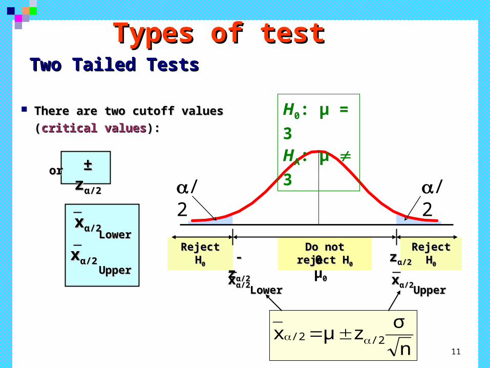
Do not reject HDo not reject H00 Reject HReject H00Reject HReject H00

There are two cutoff values There are two cutoff values

((critical valuescritical values):):

oror

Two Tailed TestsTwo Tailed Tests

/2

-z-zαα/2/2

xxαα/2/2

± ± zzαα/2/2

xxαα/2/2

0μ0

H0: μ = 3

HA: μ

3

zzαα/2/2

xxαα/2/2

n

σzμx /2/2

LowerLower

UpperUpperxxαα/2/2

LowerLower UpperUpper

/2

Types of testTypes of test

12

Errors in Making Errors in Making DecisionsDecisions

Type I ErrorType I Error Reject a true null hypothesisReject a true null hypothesis Considered a serious type of errorConsidered a serious type of error

The probability of Type I Error is The probability of Type I Error is

Called Called level of significancelevel of significance of the test of the test Set by researcher in advanceSet by researcher in advance

13

Type II ErrorType II Error Fail to reject a false null hypothesisFail to reject a false null hypothesis

The probability of Type II Error is The probability of Type II Error is ββ

(continued)Errors in Making Errors in Making DecisionsDecisions

14

Outcomes and Outcomes and ProbabilitiesProbabilities

State of NatureState of Nature

DecisionDecision

Do NotDo NotRejectReject

H0

No error (1 - )

Type II Error ( β )

RejectRejectH0

Type I Error( )

Possible Hypothesis Test OutcomesPossible Hypothesis Test Outcomes

HH00 False False HH00 True True

Key:Key:OutcomeOutcome

(Probability)(Probability) No Error ( 1 - β )

15

Critical Value Approach to Critical Value Approach to TestingTesting

Convert sample statistic (e.g.: ) to test statistic Convert sample statistic (e.g.: ) to test statistic ( ( Z or t sZ or t statistic )tatistic )

Determine the critical value(s) for a specifiedDetermine the critical value(s) for a specifiedlevel of significance level of significance from a table or computer from a table or computer

If the test statistic falls in the rejection region, If the test statistic falls in the rejection region, reject Hreject H00 ; otherwise do not reject H ; otherwise do not reject H00

x

16

Convert sample statistic ( ) to a Convert sample statistic ( ) to a test statistictest statistic ( ( Z or t sZ or t statistic )tatistic )

x

Known

Large Samples

Unknown

Hypothesis Hypothesis Tests for Tests for

Small Samples

Critical Value Approach to Critical Value Approach to TestingTesting

17

Known

Large Samples

Unknown

Hypothesis Tests for μ

Small Samples

The test statistic is:The test statistic is:

Calculating the Test Calculating the Test StatisticStatistic

n

σμx

z

18

Known

Large Samples

Unknown

Hypothesis Tests for

Small Samples

The test statistic is:The test statistic is:

n

sμx

t 1n

But is But is sometimes sometimes approximated approximated using a z:using a z:

(continued)

Calculating the Test Calculating the Test StatisticStatistic

n

μx

z

19

Known

Large Samples

Unknown

Hypothesis Tests for

Small Samples

The test statistic is:The test statistic is:

n

sμx

t 1n

(The population must be (The population must be approximately normal)approximately normal)

Calculating the Test Calculating the Test StatisticStatistic

(continued)

20

Steps in Hypothesis Steps in Hypothesis TestingTesting

1.1. Specify the population value of interestSpecify the population value of interest

2.2. Formulate the appropriate null and alternative Formulate the appropriate null and alternative hypotheseshypotheses

3.3. Specify the desired level of significanceSpecify the desired level of significance

4.4. Determine the rejection regionDetermine the rejection region

5.5. Obtain sample evidence and compute the test Obtain sample evidence and compute the test statisticstatistic

6.6. Reach a decision and interpret the resultReach a decision and interpret the result

21

Hypothesis Testing Hypothesis Testing ExampleExample

Test the claim that the true mean # of TV sets Test the claim that the true mean # of TV sets in US homes is at least 3.in US homes is at least 3.

(Assume (Assume σσ = 0.8) = 0.8)

1.1. HH00: : μμ 3 H 3 HAA: : μμ < 3 (This is a < 3 (This is a

lower tail test)lower tail test)

2.2. Suppose that Suppose that = .05 is chosen = .05 is chosen

for this testfor this test

22

Suppose a sample is taken with the following results: Suppose a sample is taken with the following results:

n = 100, x = 2.84 n = 100, x = 2.84

Then the test statistic is:Then the test statistic is:

2.0.08

.16

100

0.832.84

n

σμx

z

Hypothesis Testing Hypothesis Testing ExampleExample

But zBut ztab tab = - 1.645= - 1.645

Since -2.0 < -1.645, we Since -2.0 < -1.645, we reject the null reject the null hypothesishypothesis that the mean number of TVs in US that the mean number of TVs in US homes is at least 3 homes is at least 3

23

Upper Tail z Test for Mean (Upper Tail z Test for Mean ( Known)Known)

A phone industry manager thinks that A phone industry manager thinks that customer monthly cell phone bill have customer monthly cell phone bill have increased, and now average over $52 per increased, and now average over $52 per month. The company wishes to test this month. The company wishes to test this claim. (Assume claim. (Assume = 10 is known) = 10 is known)

HH00: : μμ ≤ 52 the average is not over $52 per month≤ 52 the average is not over $52 per month

HHAA: : μμ > 52 the average is greater than $52 per month > 52 the average is greater than $52 per month

Form hypothesis test:Form hypothesis test:

24

Suppose a sample is taken with the following results: Suppose a sample is taken with the following results: n = 64, x = 53.1 (n = 64, x = 53.1 (=10 was assumed known) =10 was assumed known)

Then the test statistic is:Then the test statistic is:

0.88

64

105253.1

n

σμx

z

(continued)(continued)

Upper Tail z Test for Mean (Upper Tail z Test for Mean ( Known)Known)

But zBut ztabtab = 1.28 = 1.28

Do not reject HDo not reject H00 since 0.88 since 0.88 ≤≤ 1.28 1.28

i.e.: there is not sufficient evidence that the mean bill is over $52i.e.: there is not sufficient evidence that the mean bill is over $52

25

Example: Two-Tail Test (Example: Two-Tail Test ( Unknown)Unknown)

The average cost of a hotel The average cost of a hotel

room in New York is said to be room in New York is said to be

$168 per night. A random $168 per night. A random

sample of 25 hotels resulted in sample of 25 hotels resulted in

x = $172.50 and x = $172.50 and

s = $15.40. Test at the s = $15.40. Test at the

= 0.05 level.= 0.05 level.

(Assume the population (Assume the population

distribution is normal)distribution is normal)

H0: μ= 168

HA: μ

168

26

= 0.05

n = 25

is unknown, so use a t statistic

Critical Value:

t24 = ± 2.0639

Example Solution: Two-Tail Test

Do not reject H0: not sufficient evidence that true mean cost is different than $168

Reject H0Reject H0

/2=.025

-tα/2

Do not reject H0

0 tα/2

/2=.025

-2.0639 2.0639

1.46

25

15.40168172.50

n

sμx

t 1n

1.46

H0: μ= 168

HA: μ

168

27

Hypothesis Tests for Proportions

Involves categorical values

Two possible outcomes

“Success” (possesses a certain characteristic)

“Failure” (does not possesses that characteristic)

Fraction or proportion of population in the “success” category is denoted by p

28

Proportions Sample proportion in the success category is

denoted by p

When both np and n(1-p) are at least 5, p can be approximated by a normal distribution with mean and standard deviation

(continued)

sizesample

sampleinsuccessesofnumber

n

xp

pμP

n

p)p(1σ

p

29

The sampling distribution of p is normal, so the test statistic is a z value:

Hypothesis Tests for Proportions

n)p(p

ppz

1

np 5and

n(1-p) 5

Hypothesis Tests for p

np < 5or

n(1-p) < 5

Not discussed in this chapter

30

Example: z Test for Proportion

A marketing company claims that it receives 8% responses from its mailing. To test this claim, a random sample of 500 were surveyed with 25 responses. Test at the = .05 significance level.

Check:

n p = (500)(.08) = 40

n(1-p) = (500)(.92) = 460

31

Z Test for Proportion: Solution

= .05

n = 500, p = .05

Reject H0 at = .05

H0: p = .08

HA: p

.08

Critical Values: ± 1.96

Test Statistic:

Decision:

Conclusion:

z0

Reject Reject

.025.025

1.96

-2.47

There is sufficient evidence to reject the company’s claim of 8% response rate.

2.47

500.08).08(1

.08.05

np)p(1

ppz

-1.96

32

Do not reject H0

Reject H0Reject H0

/2 = .025

1.960

z = -2.47

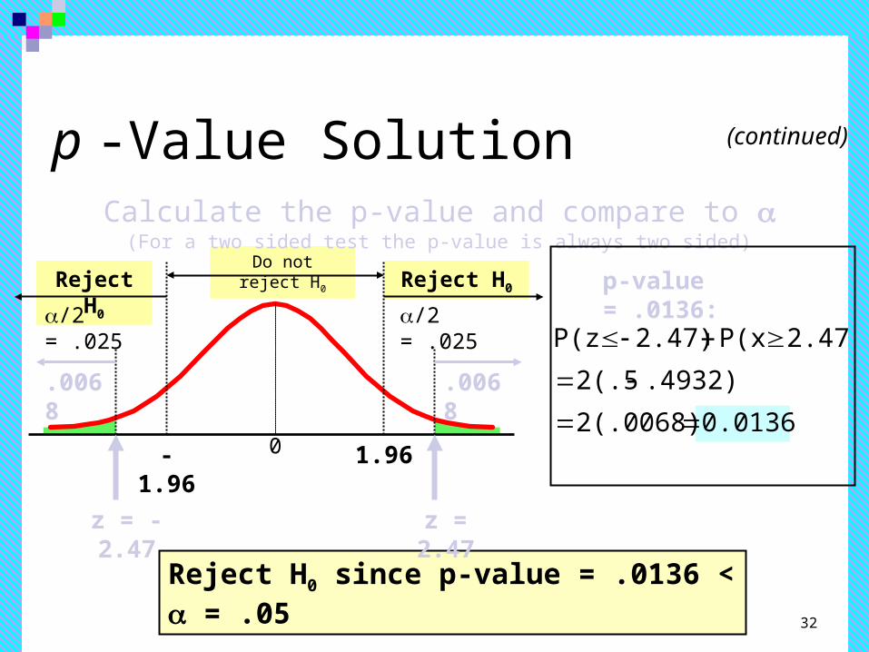
Calculate the p-value and compare to (For a two sided test the p-value is always two sided)

(continued)

0.01362(.0068)

.4932)2(.5

2.47)P(x2.47)P(z

p-value = .0136:

p -Value Solution

Reject H0 since p-value = .0136 < = .05

z = 2.47

-1.96

/2 = .025

.0068.0068

33

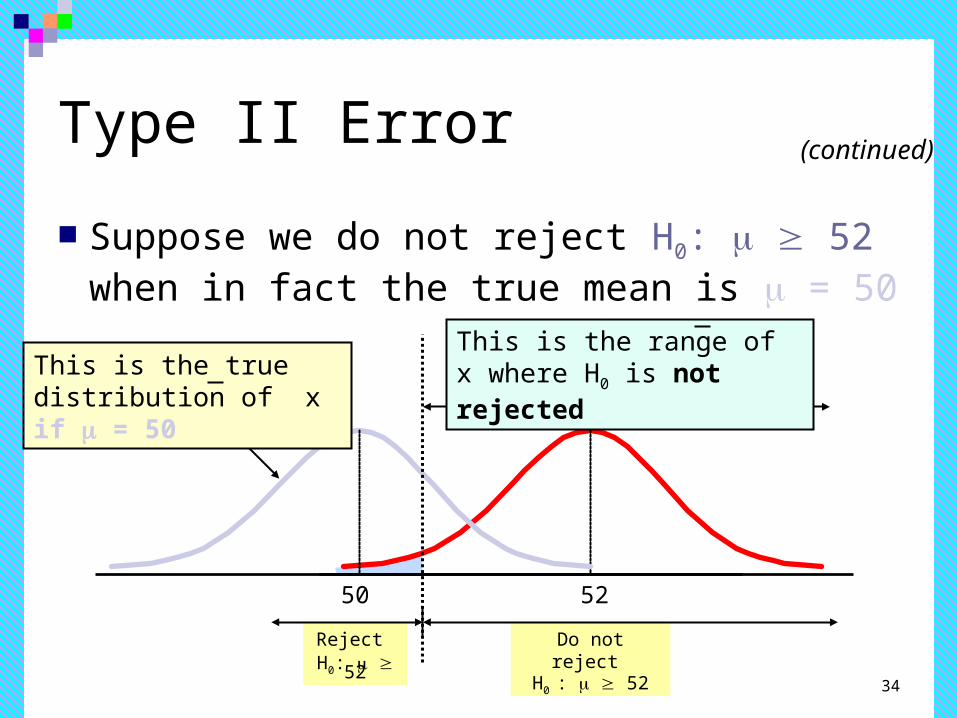
Reject H0: μ 52

Do not reject H0 : μ 52

Type II Error Type II error is the probability of

failing to reject a false H0

5250

Suppose we fail to reject H0: μ 52 when in fact the true mean is μ = 50

34

Reject H0: 52

Do not reject H0 : 52

Type II Error

Suppose we do not reject H0: 52 when in fact the true mean is = 50

5250

This is the true distribution of x if = 50

This is the range of x where H0 is not rejected

(continued)

35

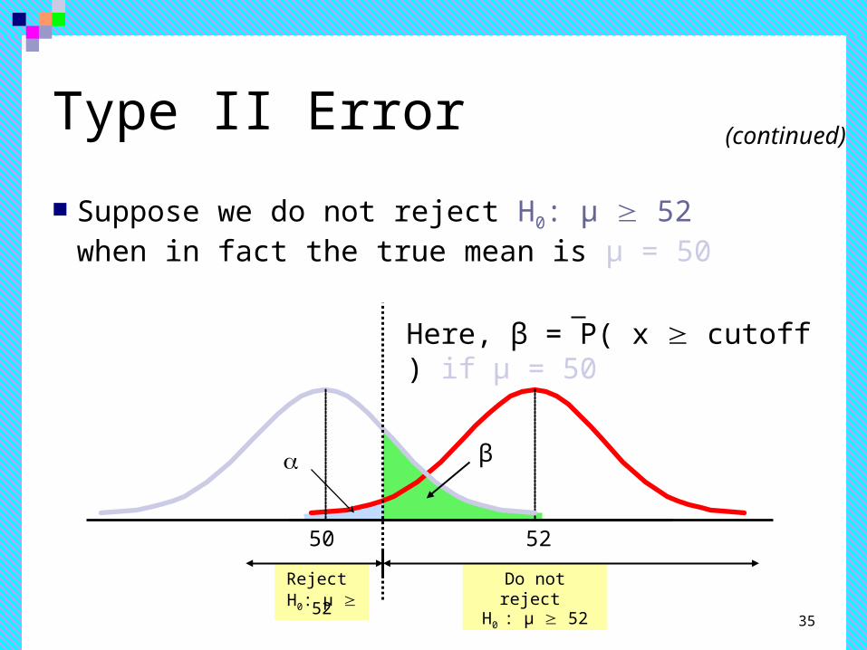
Reject H0: μ 52

Do not reject H0 : μ 52

Type II Error

Suppose we do not reject H0: μ 52 when in fact the true mean is μ = 50

5250

β

Here, β = P( x cutoff ) if μ = 50

(continued)

36

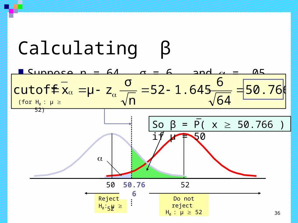
Reject H0: μ 52

Do not reject H0 : μ 52

Suppose n = 64 , σ = 6 , and = .05

5250

So β = P( x 50.766 ) if μ = 50

Calculating β

50.76664

61.64552

n

σzμxcutoff

(for H0 : μ 52)

50.766

37

Reject H0: μ 52

Do not reject H0 : μ 52

.1539.3461.51.02)P(z

646

5050.766zP50)μ|50.766xP(

Suppose n = 64 , σ = 6 , and = .05

5250

Calculating β (continued)

Probability of type II error:

β = .1539

38

Using PHStat

Options

39

Sample PHStat Output

Input

Output

40

Chapter Summary Addressed hypothesis testing methodology

Performed z Test for the mean (σ known)

Discussed p–value approach to hypothesis testing

Performed one-tail and two-tail tests . . .

41

Chapter Summary

Performed t test for the mean (σ unknown)

Performed z test for the proportion

Discussed type II error and computed its probability

(continued)