1

Introduction to biostatisticsBy

Dr. S. Shaffi AhamedAsst. Professor

Dept. of Family & Community MedicineKKUH

2

This session covers:

Background and need to know Biostatistics

Definition of Statistics and Biostatistics Types of data Frequency distribution of a data Graphical representation of a data

3

What Is Statistics?

Why?

1. Collecting Data e.g., Sample, Survey, Observe,

Simulate

2. Characterizing Data e.g., Organize/Classify, Count,

Summarize

3. Presenting Data e.g., Tables, Charts,

Statements

4. Interpreting Resultse.g. Infer, Conclude, Specify Confidence

Data Analysis

Decision-Making

© 1984-1994 T/Maker Co.

4

Statistics is the science of conducting studies to collect, organize, summarize, analyze, present, interpret and draw conclusions from data.

Any values (observations or measurements) that have been collected

5

Basis

6

Dynamic nature of the U n i v e r s e

the very continuous change in Nature brings - uncertainty

and - variability

in each and every sphere of the Universe

7

We by no mean can control or over-power

the factor of uncertainty but capable of measuring it in terms of

Probability

8

Sources of Medical Uncertainties

1. Intrinsic due to biological, environmental and sampling factors

2. Natural variation among methods, observers, instruments etc.

3. Errors in measurement or assessment or errors in knowledge

4. Incomplete knowledge

9

Biostatistics is the science that helps in managing medical uncertainties

10

“BIOSTATISICS”

(1) Statistics arising out of biological sciences, particularly from the fields of Medicine and public health.

(2) The methods used in dealing with statistics in the fields of medicine, biology and public health for planning, conducting and analyzing data which arise in investigations of these branches.

11

CLINICAL MEDICINE

Documentation of medical history of diseases.

Planning and conduct of clinical studies.Evaluating the merits of different

procedures.In providing methods for definition of

“normal” and “abnormal”.

12

PREVENTIVE MEDICINE

To provide the magnitude of any health problem in the community.

To find out the basic factors underlying the ill-health.

To evaluate the health programs which was introduced in the community (success/failure).

To introduce and promote health legislation.

13

Role of Biostatics in Health Planning and EvaluationIn carrying out a valid and reliable

health situation analysis, including in proper summarization and interpretation of data.

In proper evaluation of the achievements and failures of a health programs.

14

Role of Biostatistics in Medical ResearchIn developing a research design that

can minimize the impact of uncertaintiesIn assessing reliability and validity of

tools and instruments to collect the information

In proper analysis of data

15

BASIC CONCEPTSData : Set of values of one or more variables recorded on one or more observational units (singular: Datum)

Categories of data 1. Primary data: observation, questionnaire, record form, interviews, survey, 2. Secondary data: census, medical record,registry

Sources of data 1. Routinely kept records2. Surveys (census)3. Experiments4. External source

16

Variables and Types of DataVariables and Types of DataTo gain knowledge about seemingly haphazard events, statisticians collect information for variables, which describe the event.

Variables whose values are determined by chance are called random variables

Variables

•is a characteristic or attribute that can assume different values.

•is also a characteristics of interest, one that can be expressed as a number that possessed by each item under study.

•The value of this characteristics is likely to change or vary from one item in the data set to the next.

17

Variables can be classified

By how they are categorized, counted

or measured - Level of

measurements of data

As Quantitative and Qualitative

18

Nomenclature

Nominal variable: Variable consists of named categories with

no implied order among them. Has cancer or notReceived treatment or did notIs alive or dead

Is coded (male = 1, female = 2) but has no quantitative value.

19

Nomenclature (cont.)

Ordinal variable: Variable consists of ordered categories and

differences between categories are not equal. Patient status (Improved / Same / Worse)Diagnosis (Stage I / Stage II / Stage III) Evaluation (Satisfied / neutral / Dissatisfied)

The coding now has meaning: Improved = 2, Same = 1, worse = 0However, distance between values is not

a constant.

20

Other Nomenclature (cont.)Interval variable:

Variable has equal distances between values but the zero point is arbitrary. IQ 70 to 80 same as IQ 90 to 100.IQ scale could convert 100 to 500 and have

same meaning. IQ of 100 is not twice as smart as IQ of 50.

Temperature (37º C -- 36º C; 38º C-- 37º C are equal) and

No implication of ratio (30º C is not twice as hot as 15º C)

21

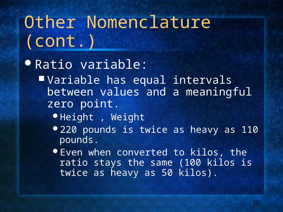
Other Nomenclature (cont.)

Ratio variable: Variable has equal intervals between

values and a meaningful zero point. Height , Weight220 pounds is twice as heavy as 110 pounds.Even when converted to kilos, the ratio stays

the same (100 kilos is twice as heavy as 50 kilos).

22

Scales of Measurement

QualitativeQualitativeQualitativeQualitative QuantitativQuantitativee

QuantitativQuantitativee

NumericalNumericalNumericalNumerical NumericalNumericalNumericalNumericalNonnumericalNonnumericalNonnumericalNonnumerical

DataDataDataData

NominaNominallNominaNominall

OrdinaOrdinallOrdinaOrdinall

NominalNominalNominalNominal OrdinalOrdinalOrdinalOrdinal IntervalIntervalIntervalInterval RatioRatioRatioRatio

23

Level of Measurements of Data Level of Measurements of Data

Nominal-level data

Ordinal-level data

Interval-level data

Ratio-level data

classifies data into mutually exclusive (non overlapping), exhausting

categories in which no order or

ranking can be imposed on the

data

classifies data into categories

that can be ranked;

however, precise differences between the ranks do not

exist

ranks data, and

precise differences

between units of measure do exist; however, there is

no meaningful zero

Possesses all the characteristics of

interval measurement,

and there exists a true zero.

Examples

24

Discrete data -- Gaps between possible values

Continuous data -- Theoretically,no gaps between possible values

Number of Children

Hb

25

CONTINUOUS DATA QUALITATIVE DATA

wt. (in Kg.) : under wt, normal & over wt. Ht. (in cm.): short, medium & tall

2626

hospital length of stay Number Percent

1 – 3 days 5891 43.3

4 – 7 days 3489 25.6

2 weeks 2449 18.0

3 weeks 813 6.0

1 month 417 3.1

More than 1 month 545 4.0

Total 14604 100.0

Mean = 7.85 SE = 0.10

Table 1 Distribution of blunt injured patients according to hospital length of stay

27

CLINIMETRICSA science called clinimetrics in which

qualities are converted to meaningful quantities by using the scoring system.

Examples: (1) Apgar score based on appearance, pulse, grimace, activity and respiration is used for neonatal prognosis.

(2) Smoking Index: no. of cigarettes, duration, filter or not, whether pipe, cigar etc.,

(3) APACHE( Acute Physiology and Chronic Health Evaluation) score: to quantify the severity of condition of a patient

30

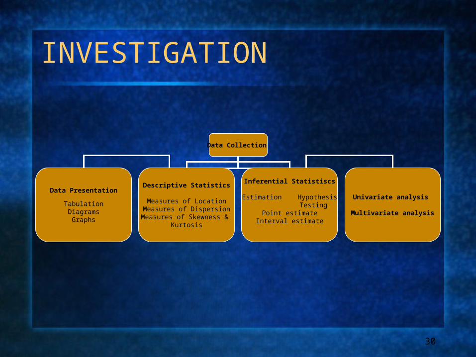
INVESTIGATION

Data Collection

Data Presentation

TabulationDiagramsGraphs

Descriptive Statistics

Measures of LocationMeasures of Dispersion

Measures of Skewness & Kurtosis

Inferential Statistiscs

Estimation Hypothesis TestingPoint estimate

Interval estimate

Univariate analysis

Multivariate analysis

31

An overview of descriptive An overview of descriptive statistics and statistical inferencestatistics and statistical inference

START

Gathering of Data

Classification, Summarization, and Processing of data

Presentation and Communication of

Summarized information

Is Information from a sample?

Use cencus data to analyze the population

characteristic under study

Use sample information to make inferences about

the population

Draw conclusions about the population

characteristic (parameter) under study

STOP

Yes

No

Statistical Inference

Descriptive

Statistics

Statistical Inference

Descriptive Statistics

No

Yes

32

Descriptive & Inferential StatisticsDescriptive & Inferential Statistics

Inferential statisticsInferential statistics

consists of generalizing from samples to populations, performing estimations hypothesis testing, determining relationships among variables, and making predictions.

Used when we want to draw a conclusion for the data obtain from the sample

Used to describe, infer, estimate, approximate the characteristics of the target population

Descriptive statisticsDescriptive statistics

consists of the collection, organization, classification, summarization, and presentation of data obtain from the sample.

Used to describe the characteristics of the sample

Used to determine whether the sample represent the target population by comparing sample statistic and population parameter

33

Frequency Distributions“A Picture is Worth a Thousand Words”

34

Frequency Distributions

data distribution – pattern of variability. the center of a distribution the ranges the shapes

simple frequency distributionsgrouped frequency distributions

35

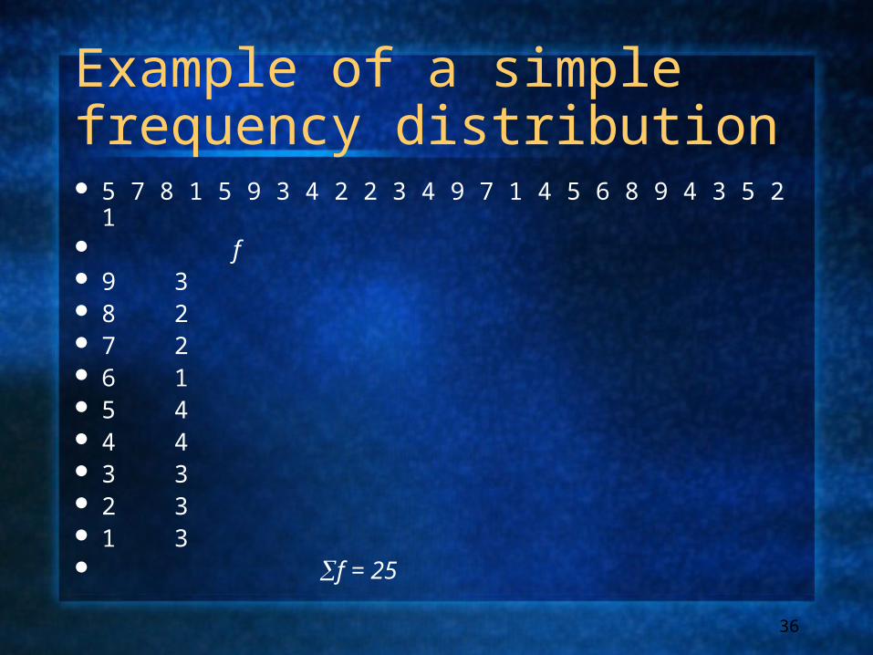
Simple Frequency Distribution

The number of times that score occursMake a table with highest score at top

and decreasing for every possible whole number

N (total number of scores) always equals the sum of the frequency f = N

36

Example of a simple frequency distribution 5 7 8 1 5 9 3 4 2 2 3 4 9 7 1 4 5 6 8 9 4 3 5 2 1 f 9 3 8 2 7 2 6 1 5 4 4 4 3 3 2 3 1 3 f = 25

37

Relative Frequency Distribution

Proportion of the total NDivide the frequency of each score by NRel. f = f/NSum of relative frequencies should

equal 1.0Gives us a frame of reference

38

Example of a simple frequency distribution 5 7 8 1 5 9 3 4 2 2 3 4 9 7 1 4 5 6 8 9 4 3 5 2 1 f rel f 9 3 .12 8 2 .08 7 2 .08 6 1 .04 5 4 .16 4 4 .16 3 3 .12 2 3 .12 1 3 .12 f = 25 rel f = 1.0

39

Cumulative Frequency Distributions

cf = cumulative frequency: number of scores at or below a particular score

A score’s standing relative to other scores

Count from lower scores and add the simple frequencies for all scores below that score

40

Example of a simple frequency distribution 5 7 8 1 5 9 3 4 2 2 3 4 9 7 1 4 5 6 8 9 4 3 5 2 1 f rel f cf 9 3 .12 3 8 2 .08 5 7 2 .08 7 6 1 .04 8 5 4 .16 12 4 4 .16 16 3 3 .12 19 2 3 .12 22 1 3 .12 25 f = 25 rel f = 1.0

41

Patient No

Hb(g/dl)

Patient No

Hb(g/dl)

Patient No

Hb(g/dl)

1 12.0 11 11.2 21 14.9

2 11.9 12 13.6 22 12.2

3 11.5 13 10.8 23 12.2

4 14.2 14 12.3 24 11.4

5 12.3 15 12.3 25 10.7

6 13.0 16 15.7 26 12.5

7 10.5 17 12.6 27 11.8

8 12.8 18 9.1 28 15.1

9 13.2 19 12.9 29 13.4

10 11.2 20 14.6 30 13.1

Tabulate the hemoglobin values of 30 adult Tabulate the hemoglobin values of 30 adult male patients listed belowmale patients listed below

42

Steps for making a table

Step1 Find Minimum (9.1) & Maximum (15.7)

Step2 Calculate difference 15.7 – 9.1 = 6.6

Step3 Decide the number and width of the classes (7 c.l) 9.0 -9.9, 10.0-10.9,----

Step4 Prepare dummy table – Hb (g/dl), Tally mark, No. patients

43

Hb (g/dl) Tall marks No. patients

9.0 – 9.910.0 – 10.911.0 – 11.912.0 – 12.913.0 – 13.914.0 – 14.915.0 – 15.9

   

Total    

   Hb (g/dl) Tall marks No.

patients

9.0 – 9.910.0 – 10.911.0 – 11.9

12.0 – 12.913.0 – 13.9

14.0 – 14.9

15.0 – 15.9

llll llll 1llll llll

lllllll

ll

136105

3

2Total - 30

DUMMY TABLEDUMMY TABLE Tall Marks TABLETall Marks TABLE

44

Hb (g/dl) No. of patients

9.0 – 9.910.0 – 10.911.0 – 11.912.0 – 12.913.0 – 13.914.0 – 14.915.0 – 15.9

136

10532

Total 30

Table Frequency distribution of 30 adult male Table Frequency distribution of 30 adult male patients by Hb patients by Hb

45

Table Frequency distribution of adult patients byTable Frequency distribution of adult patients by Hb and gender:Hb and gender:

Hb(g/dl)

Gender Total

Male Female

<9.09.0 – 9.9

10.0 – 10.911.0 – 11.912.0 – 12.913.0 – 13.914.0 – 14.915.0 – 15.9

0136

10532

23586420

248

1416952

Total 30 30 60

46

Elements of a TableElements of a TableIdeal table should have Number

Title Column headings Foot-notes

Number – Table number for identification in a report

Title,place - Describe the body of the table, variables, Time period (What, how classified, where and when)

Column - Variable name, No. , Percentages (%), etc.,Heading

Foot-note(s) - to describe some column/row headings, special cells, source, etc.,

47

DIAGRAMS/GRAPHS

Qualitative data (Nominal & Ordinal) --- Bar charts (one or two groups)

Quantitative data (discrete & continuous) --- Histogram --- Frequency polygon (curve) --- Stem-and –leaf plot --- Box-and-whisker plot

48

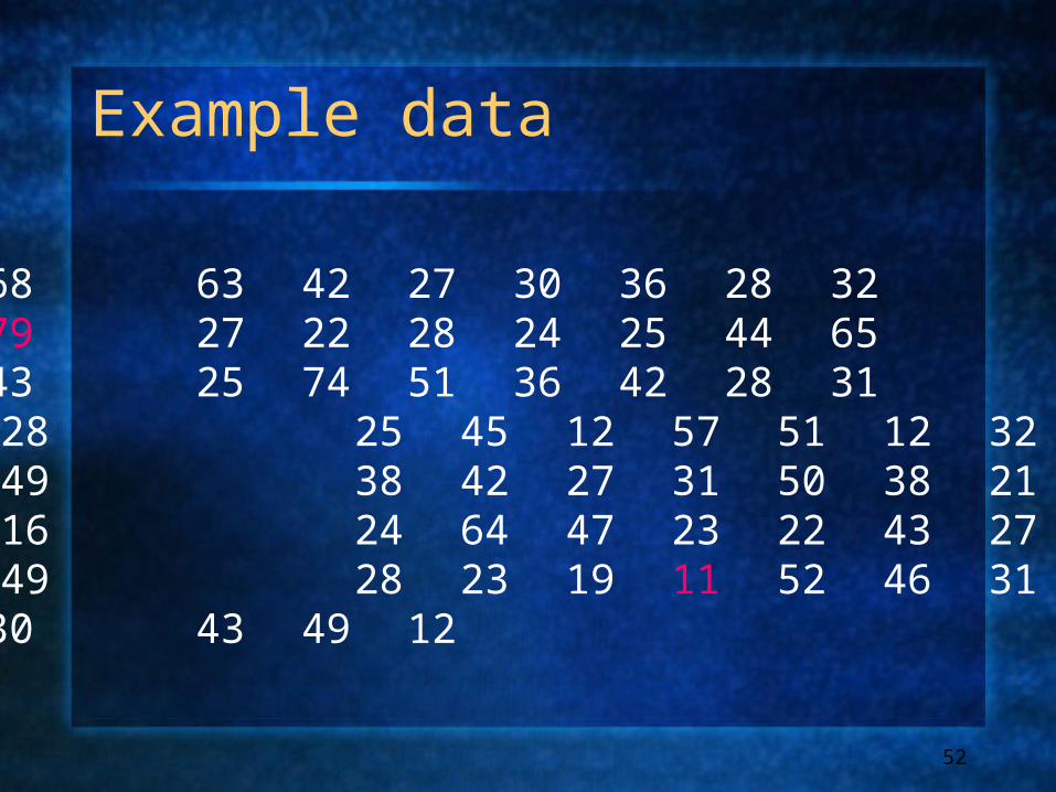
Example data

68 63 42 27 30 36 28 3279 27 22 28 24 25 44 6543 25 74 51 36 42 28 31 28 25 45 12 57 51 12 32 49 38 42 27 31 50 38 21 16 24 64 47 23 22 43 27 49 28 23 19 11 52 46 3130 43 49 12

49

Histogram

Figure 1 Histogram of ages of 60 subjects

11.5 21.5 31.5 41.5 51.5 61.5 71.5

0

10

20

Age

Freq

uen

cy

50

Polygon

71.561.551.541.531.521.511.5

20

10

0

Age

Freq

uen

cy

51

Cumulative Frequency Polygon

Cumulative counts can be converted to percents.

Shows number cases up to & including all within the interval.

%

#Common in vital statistics

50

30

52

Example data

68 63 42 27 30 36 28 3279 27 22 28 24 25 44 6543 25 74 51 36 42 28 31 28 25 45 12 57 51 12 32 49 38 42 27 31 50 38 21 16 24 64 47 23 22 43 27 49 28 23 19 11 52 46 3130 43 49 12

53

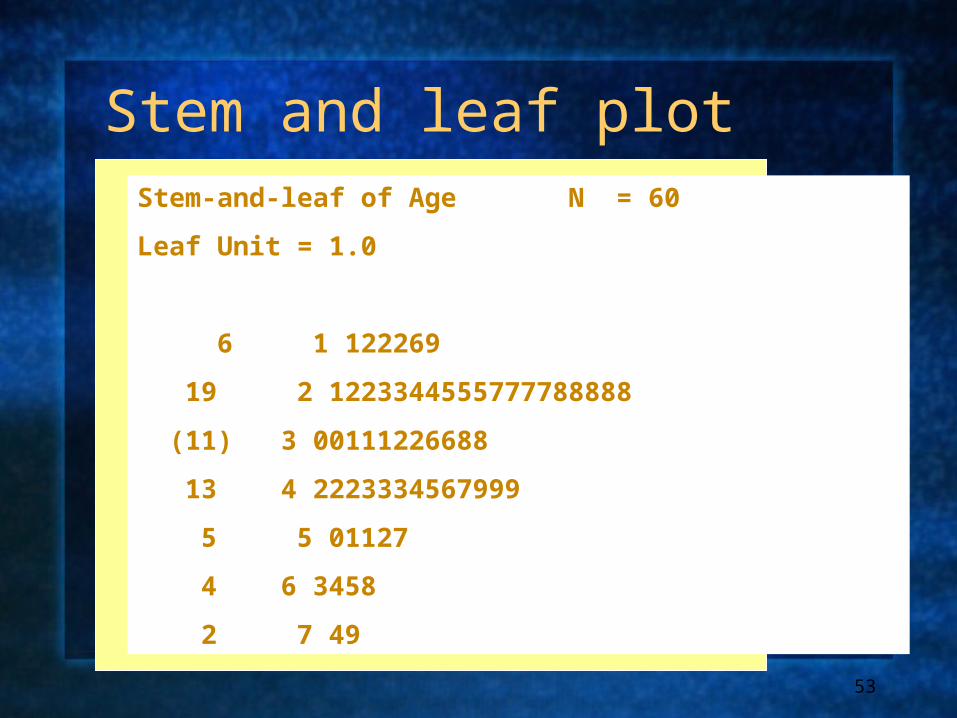
Stem and leaf plotStem-and-leaf of Age N = 60

Leaf Unit = 1.0

6 1 122269

19 2 1223344555777788888

(11) 3 00111226688

13 4 2223334567999

5 5 01127

4 6 3458

2 7 49

54

Box plot

10

20

30

40

50

60

70

80A

ge

55

Descriptive statistics report: Boxplot

- minimum score- maximum score- lower quartile- upper quartile - median- mean

- the skew of the distribution: positive skew: mean > median & high-score whisker is longer negative skew: mean < median & low-score whisker is longer

56

Application of a box and Whisker diagram

57

10%

20%

70%

Mild

Moderate

Severe

The prevalence of different degree of Hypertension

in the population

Pie Chart•Circular diagram – total -100%

•Divided into segments each representing a category

•Decide adjacent category

•The amount for each category is proportional to slice of the pie

58

Bar Graphs

912

2016

128

20

0

5

10

15

20

25

Smo Alc Chol DM HTN NoExer

F-H

Risk factor

Numb

er

The distribution of risk factor among cases with Cardio vascular Diseases

Heights of the bar indicates frequency

Frequency in the Y axis and categories of variable in the X axis

The bars should be of equal width and no touching the other bars

59

HIV cases enrolment in USA by gender

0

2

4

6

8

10

12

1986 1987 1988 1989 1990 1991 1992

Year

En

rollm

ent

(hu

nd

red

)

MenWomen

Bar chart

60

HIV cases Enrollment in USA by gender

0

2

4

6

8

10

12

14

16

18

1986 1987 1988 1989 1990 1991 1992

Year

Enro

llm

ent (T

hou

sands)

WomenMen

Stocked bar chart

61

Graphic Presentation of Data

the histogram (quantitative data)

the bar graph (qualitative data)

the frequency polygon (quantitative data)

62

63

General rules for designing graphs

A graph should have a self-explanatory legend

A graph should help reader to understand data

Axis labeled, units of measurement indicated

Scales important. Start with zero (otherwise // break)

Avoid graphs with three-dimensional impression, it may be misleading (reader visualize less easily

64

Any Questions