1 introduction to algorithms 6.046j/18.401j/sma5503 lecture 18 prof. erik demaine
TRANSCRIPT
1
Introduction to Algorithms6.046J/18.401J/SMA5503
Lecture 18Prof. Erik Demaine
2
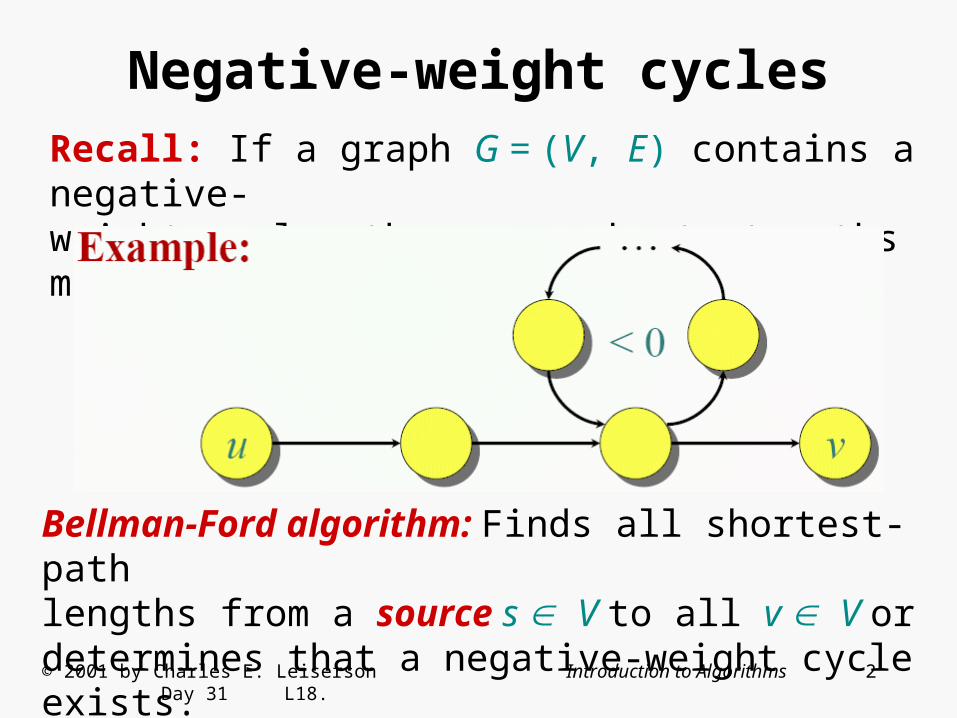
Negative-weight cyclesRecall: If a graph G = (V, E) contains a negative-weight cycle, then some shortest paths may not exist.
Bellman-Ford algorithm: Finds all shortest-pathlengths from a source s V to all v V ordetermines that a negative-weight cycle exists.
© 2001 by Charles E. Leiserson Introduction to Algorithms Day 31 L18.
3
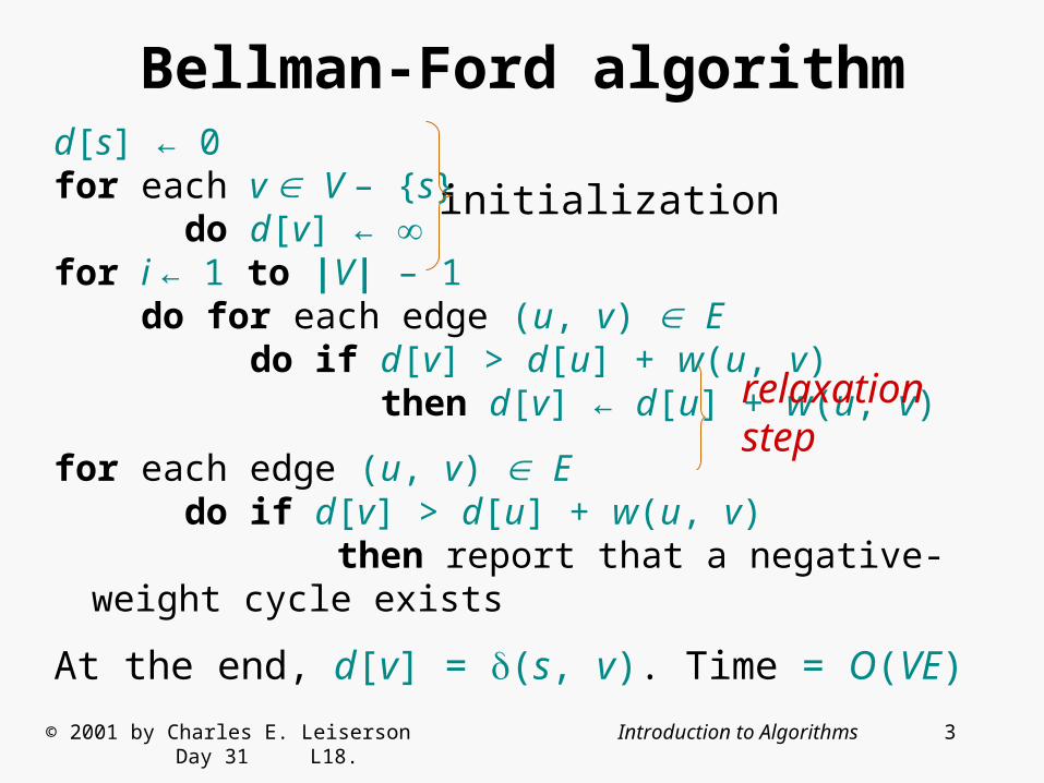
Bellman-Ford algorithmd[s] ← 0for each v V – {s} do d[v] ← for i ← 1 to |V| – 1 do for each edge (u, v) E do if d[v] > d[u] + w(u, v) then d[v] ← d[u] + w(u, v)
for each edge (u, v) E do if d[v] > d[u] + w(u, v) then report that a negative-weight cycle exists
At the end, d[v] = (s, v). Time = O(VE)
initialization
relaxationstep
© 2001 by Charles E. Leiserson Introduction to Algorithms Day 31 L18.
4
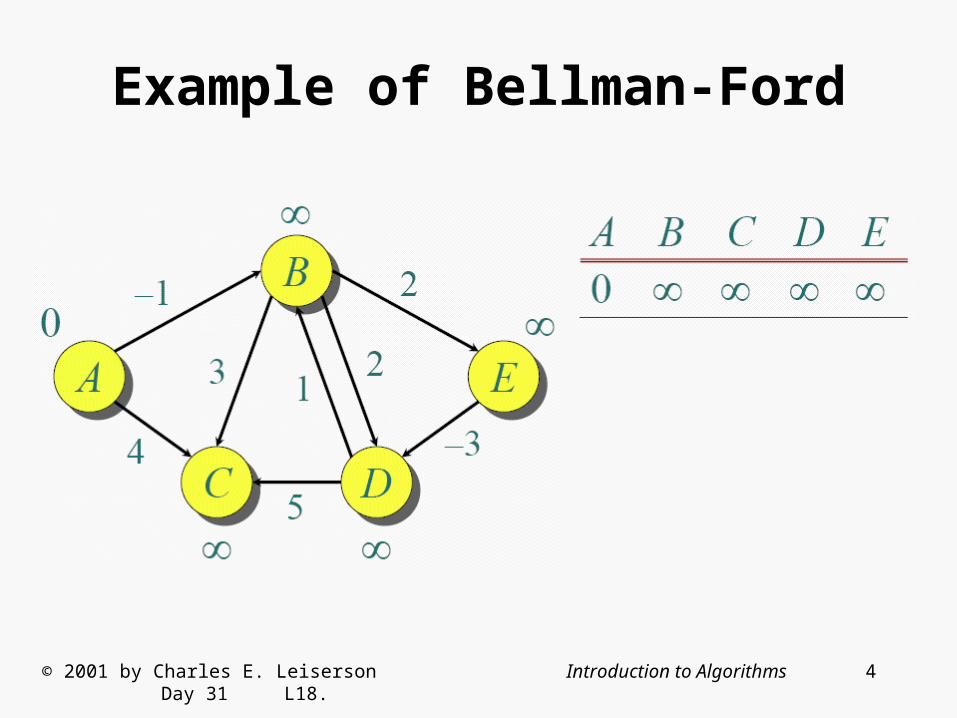
Example of Bellman-Ford
© 2001 by Charles E. Leiserson Introduction to Algorithms Day 31 L18.
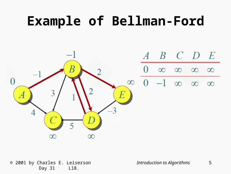
5
Example of Bellman-Ford
© 2001 by Charles E. Leiserson Introduction to Algorithms Day 31 L18.

6
Example of Bellman-Ford
© 2001 by Charles E. Leiserson Introduction to Algorithms Day 31 L18.
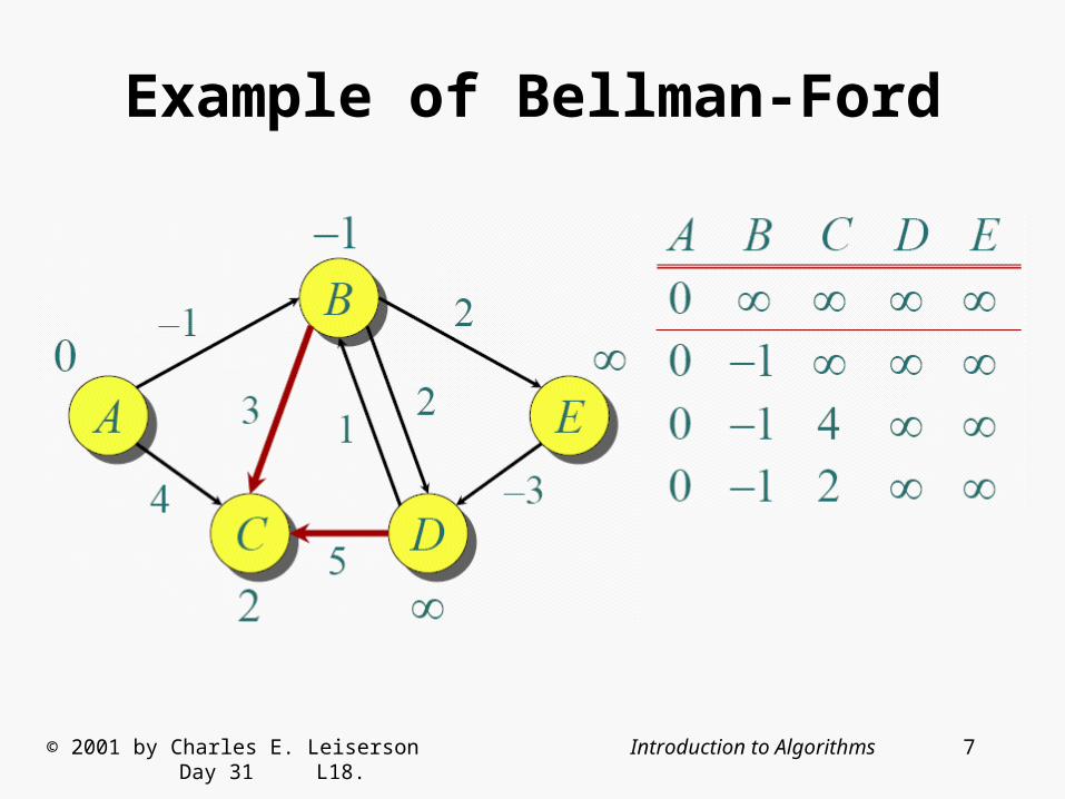
7
Example of Bellman-Ford
© 2001 by Charles E. Leiserson Introduction to Algorithms Day 31 L18.
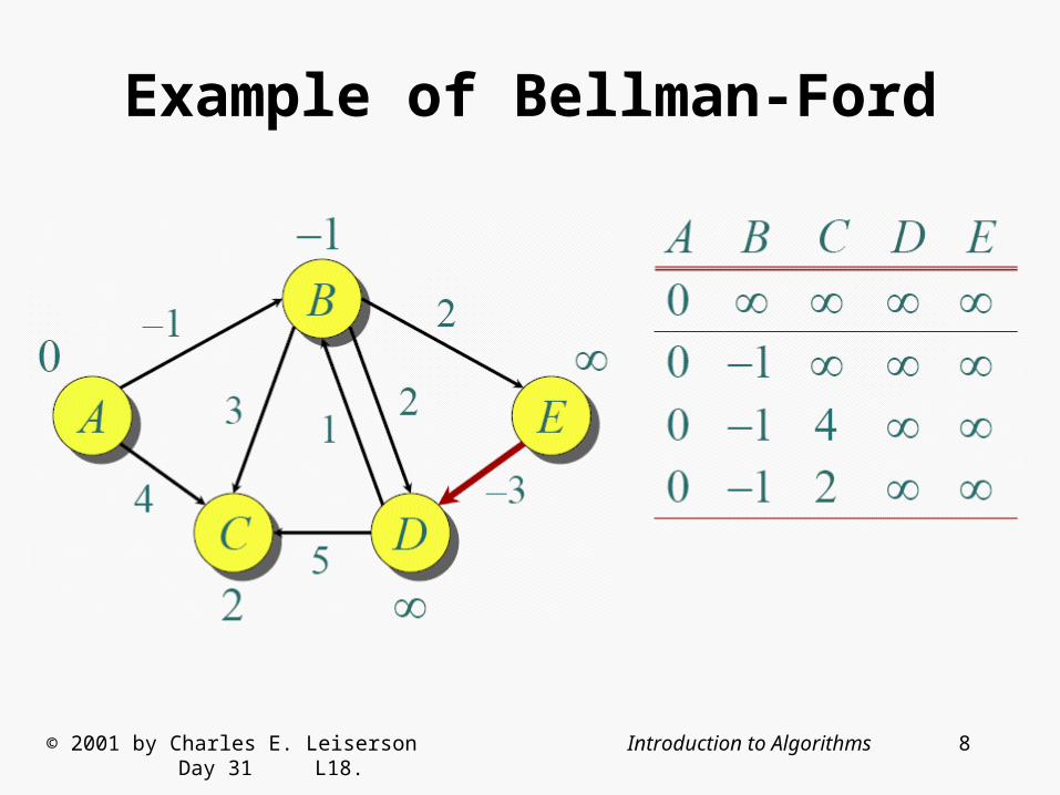
8
Example of Bellman-Ford
© 2001 by Charles E. Leiserson Introduction to Algorithms Day 31 L18.
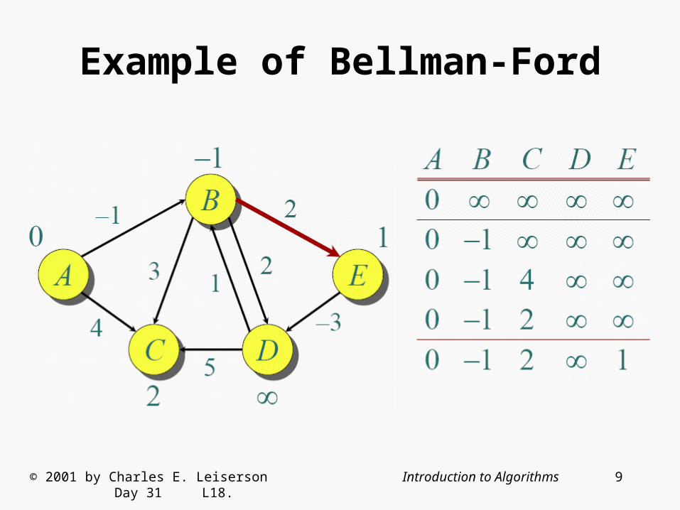
9
Example of Bellman-Ford
© 2001 by Charles E. Leiserson Introduction to Algorithms Day 31 L18.
10
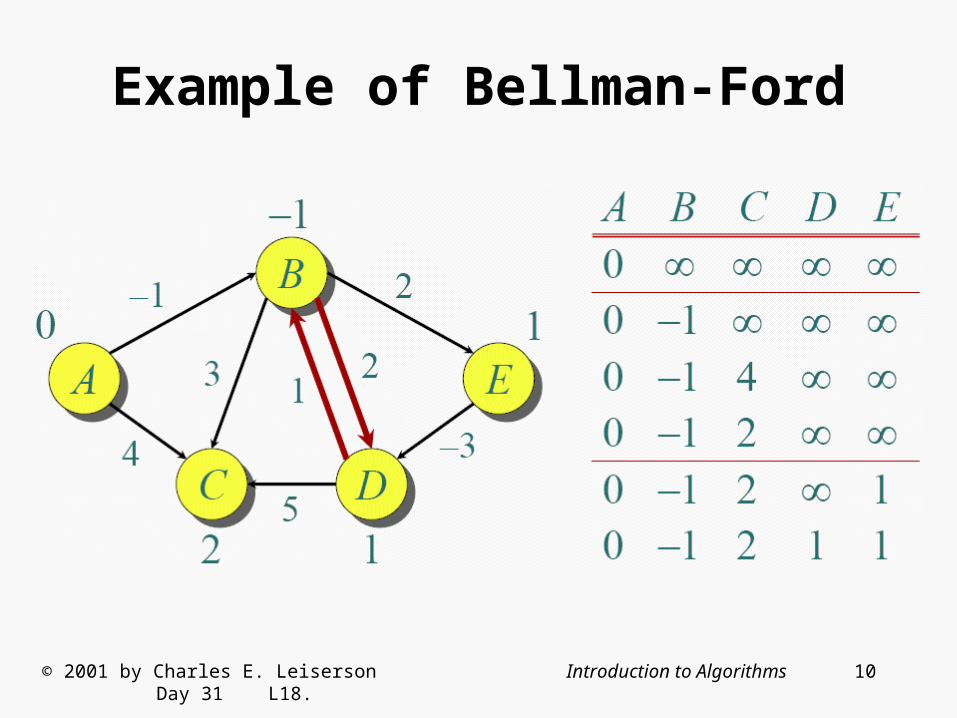
Example of Bellman-Ford
© 2001 by Charles E. Leiserson Introduction to Algorithms Day 31 L18.
11
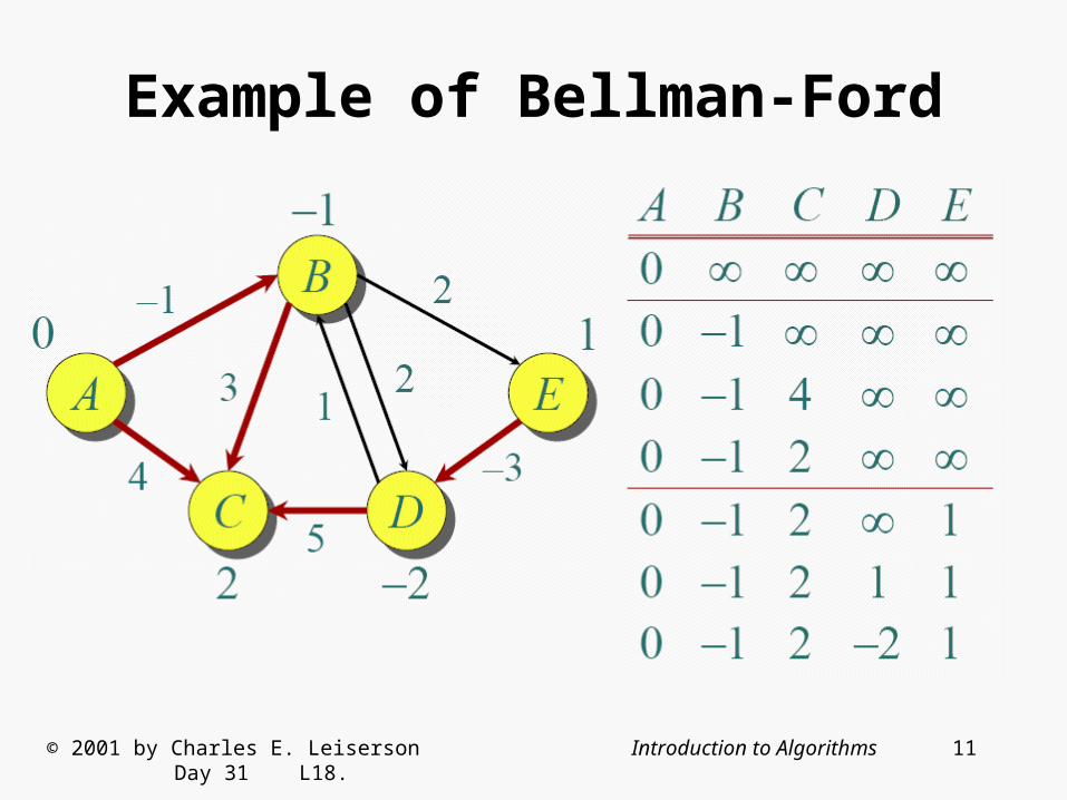
Example of Bellman-Ford
© 2001 by Charles E. Leiserson Introduction to Algorithms Day 31 L18.
12
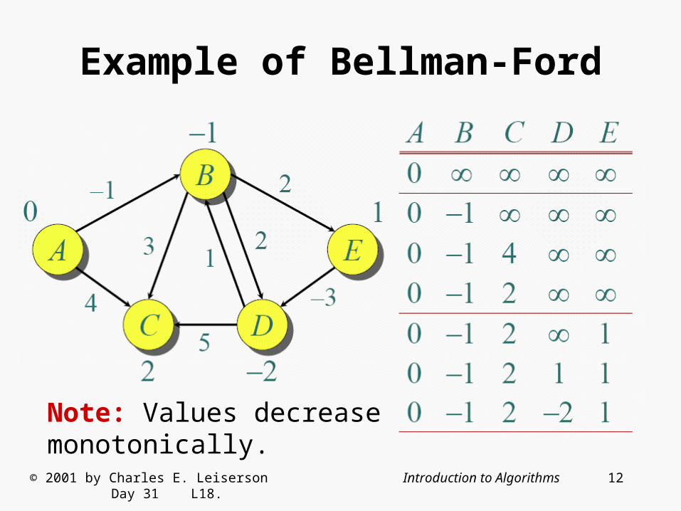
Example of Bellman-Ford
Note: Values decreasemonotonically.
© 2001 by Charles E. Leiserson Introduction to Algorithms Day 31 L18.

13
Correctness
Theorem. If G = (V, E) contains no negative-weight cycles, then after the Bellman-Fordalgorithm executes, d[v] = (s, v) for all v V.Proof. Let v V be any vertex, and consider a shortestpath p from s to v with the minimum number of edges.
Since p is a shortest path, we have
(s, vi) = (s, vi-1) + w(vi-1 , vi) .
© 2001 by Charles E. Leiserson Introduction to Algorithms Day 31 L18.
14
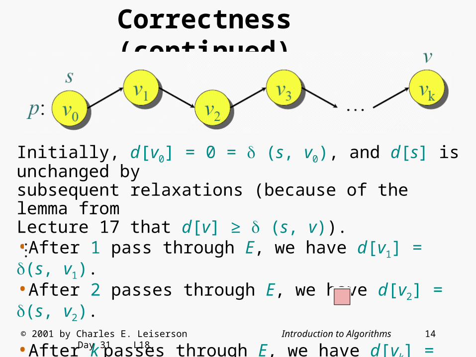
Correctness (continued)
Initially, d[v0] = 0 = (s, v0), and d[s] is unchanged bysubsequent relaxations (because of the lemma fromLecture 17 that d[v] ≥ (s, v)).•After 1 pass through E, we have d[v1] = (s, v1).•After 2 passes through E, we have d[v2] = (s, v2).
•After k passes through E, we have d[vk] = (s, vk).Since G contains no negative-weight cycles, p is simple.Longest simple path has ≤|V| – 1 edges.© 2001 by Charles E. Leiserson Introduction to Algorithms Day 31 L18.

15
Detection of negative-weightcycles
Corollary. If a value d[v] fails to converge after|V| – 1 passes, there exists a negative-weightcycle in G reachable from s.
© 2001 by Charles E. Leiserson Introduction to Algorithms Day 31 L18.
16
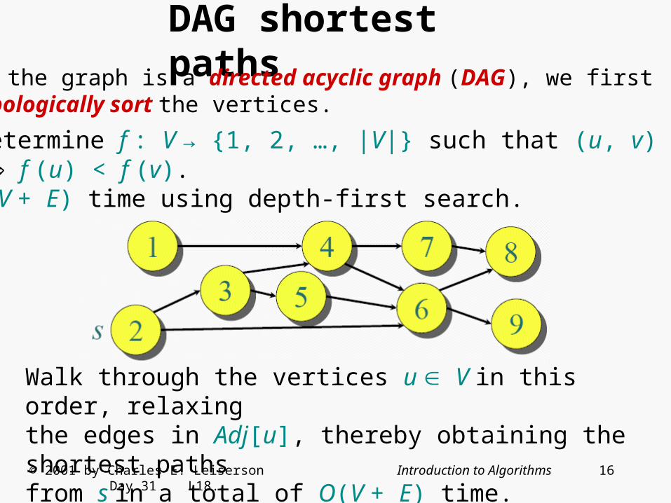
DAG shortest pathsIf the graph is a directed acyclic graph (DAG), we firsttopologically sort the vertices.
• Determine f : V → {1, 2, …, |V|} such that (u, v) E f (u) < f (v).• O(V + E) time using depth-first search.
Walk through the vertices u V in this order, relaxingthe edges in Adj[u], thereby obtaining the shortest pathsfrom s in a total of O(V + E) time.© 2001 by Charles E. Leiserson Introduction to Algorithms Day 31 L18.
17
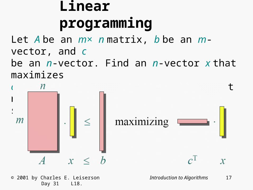
Linear programming
Let A be an m× n matrix, b be an m-vector, and cbe an n-vector. Find an n-vector x that maximizescTx subject to Ax ≤ b, or determine that no suchsolution exists.
© 2001 by Charles E. Leiserson Introduction to Algorithms Day 31 L18.

18
Linear-programmingalgorithms
Algorithms for the general problem• Simplex methods — practical, but worst-case exponential time.• Ellipsoid algorithm — polynomial time, but slow in practice.• Interior-point methods — polynomial time and competes with simplex.
Feasibility problem: No optimization criterion.Just find x such that Ax ≤ b.• In general, just as hard as ordinary LP.
© 2001 by Charles E. Leiserson Introduction to Algorithms Day 31 L18.

19
Solving a system of differenceconstraints
Linear programming where each row of A containsexactly one 1, one –1, and the rest 0’s.
Example: Solution:
Constraint graph: (The “A”matrix hasdimensions|E| × |V|.)
© 2001 by Charles E. Leiserson Introduction to Algorithms Day 31 L18.
x1 – x2 ≤ 3x2 – x3 ≤ –2x1 – x3 ≤ 2
xj – xi ≤ wij
x1 = 3x2 = 0x3 = 2
xj – xi ≤ wij
20
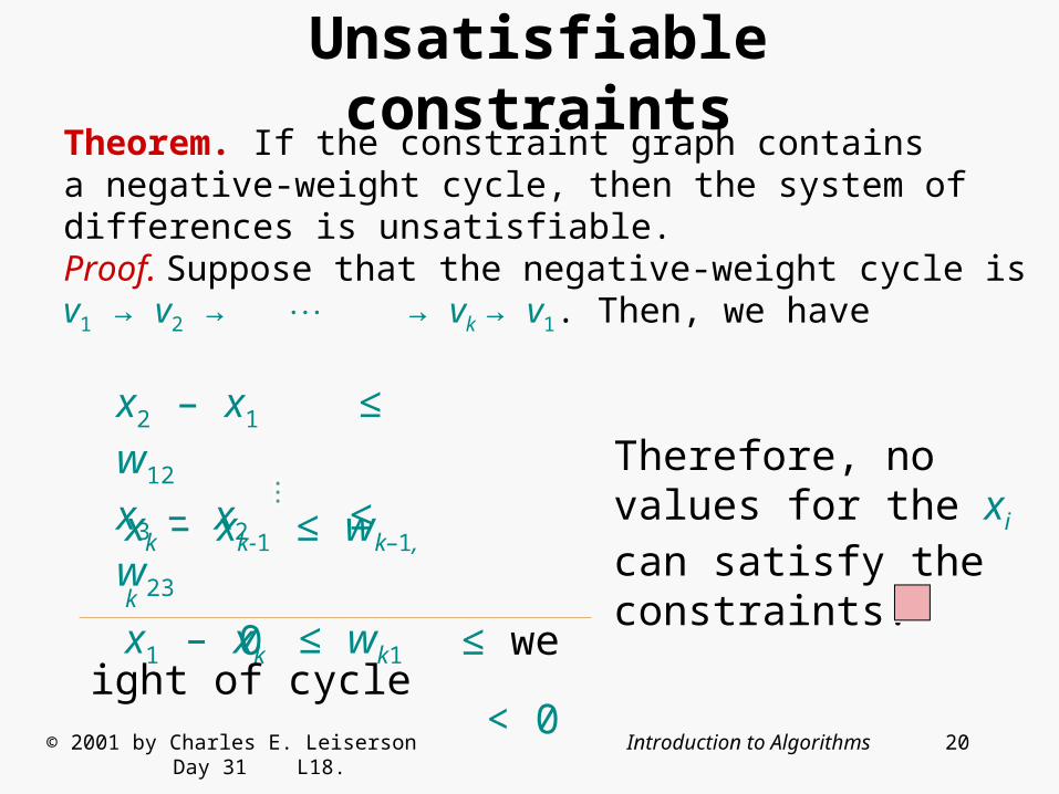
Unsatisfiable constraintsTheorem. If the constraint graph containsa negative-weight cycle, then the system ofdifferences is unsatisfiable.Proof. Suppose that the negative-weight cycle isv1 → v2 → → vk → v1. Then, we have
Therefore, novalues for the xi
can satisfy theconstraints.
© 2001 by Charles E. Leiserson Introduction to Algorithms Day 31 L18.
x2 – x1 ≤ w12
x3 – x2 ≤ w23
xk – xk-1 ≤ wk–1, k
x1 – xk ≤ wk1
0 ≤ weight of cycle < 0
21
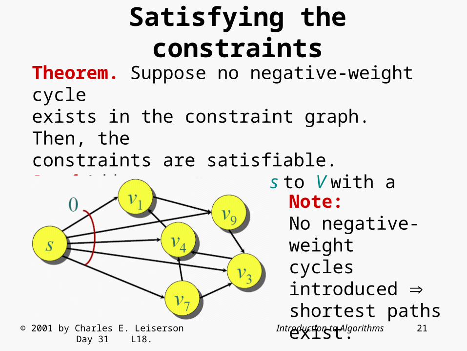
Satisfying the constraints
Theorem. Suppose no negative-weight cycleexists in the constraint graph. Then, theconstraints are satisfiable.Proof. Add a new vertex s to V with a 0-weight edgeto each vertex vi V.
Note:No negative-weightcycles introduced shortest paths exist.
© 2001 by Charles E. Leiserson Introduction to Algorithms Day 31 L18.
22
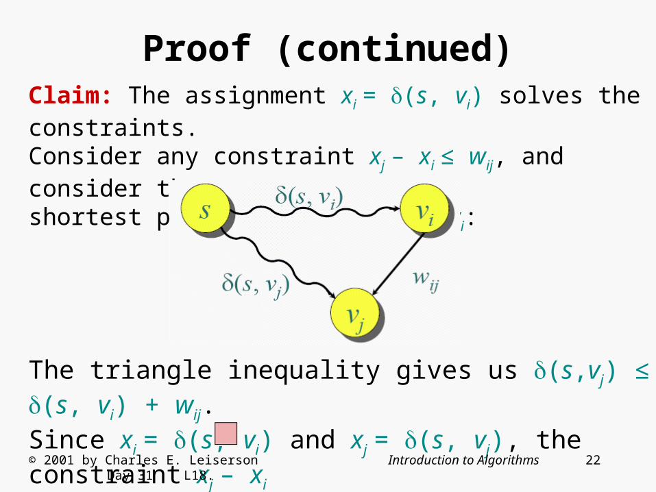
Proof (continued)Claim: The assignment xi = (s, vi) solves the constraints.Consider any constraint xj – xi ≤ wij, and consider theshortest paths from s to vj and vi:
The triangle inequality gives us (s,vj) ≤ (s, vi) + wij.Since xi = (s, vi) and xj = (s, vj), the constraint xj – xi
≤ wij is satisfied.© 2001 by Charles E. Leiserson Introduction to Algorithms Day 31 L18.

23
Bellman-Ford and linearprogramming
Corollary. The Bellman-Ford algorithm cansolve a system of m difference constraints on nvariables in O(mn) time.
Single-source shortest paths is a simple LPproblem.
In fact, Bellman-Ford maximizes x1 + x2 + + xn
subject to the constraints xj – xi ≤ wij and xi ≤ 0(exercise).
Bellman-Ford also minimizes maxi{xi} – mini{xi}(exercise).
© 2001 by Charles E. Leiserson Introduction to Algorithms Day 31 L18.
…

24
Application to VLSI layoutcompaction
Integrated-circuitfeatures:
minimum separation λ
Problem: Compact (in one dimension) thespace between the features of a VLSI layoutwithout bringing any features too close together.
© 2001 by Charles E. Leiserson Introduction to Algorithms Day 31 L18.
25
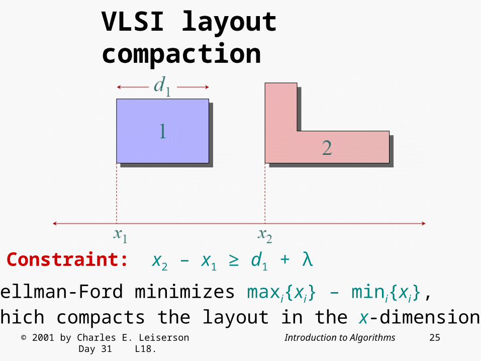
VLSI layout compaction
Constraint: x2 – x1 ≥ d1 + λ
Bellman-Ford minimizes maxi{xi} – mini{xi},which compacts the layout in the x-dimension.
© 2001 by Charles E. Leiserson Introduction to Algorithms Day 31 L18.