1. introduction, descriptors and correspondence -...

G. Quénot 1

1. Introduction, descriptors and correspondence

Georges QuénotMultimedia Information Indexing and Retrieval Group

HMUL8R6B: Information RetrievalMultimedia Indexing and Retrieval

Laboratory of Informatics of Grenoble

March 2017

G. Quénot 2

Multimedia Retrieval

• User need → retrieved documents• Images, audio, video• Retrieval of full documents or passages (e.g. shots)

• Search paradigms:– Surrounding text → may be missing, inaccurate or incomplete– Query by example → need for what you are precisely looking for– Content based search (using keywords or concepts) → need for content-based indexing → “semantic gap problem”

– Combinations including feedback

• Need for specific interfaces

G. Quénot 3

The “semantic gap”

“... the lack of coincidence between the information that one can extract from the visual data and the interpretation that the same data have for a user in a given situation” [Smeulders et al., 2002].

G. Quénot 4

The “semantic gap” problem

FaceWomanHatLena…

122 112 98 85 …

126 116 102 89 …

131 121 106 95 …

134 125 110 99 …

… … … … …

?

G. Quénot 5

“Signal” level

• Signal :– Variable in time, in space and/or in other physical

dimensions,– Analog : physical phenomenon (pressure of an acoustic

wave or distribution of light intensity) or its modeling by another one (electronic or chemical for example),

– Digital : same content but “discretized” of the value, of time, of space, and/or others (light frequency for example).

G. Quénot 6

“Signal” level

• Signal, examples :– Sound (monophonic) : values sampled at 16 kHz on 16 bits

(one temporal dimension, zero spatial dimensions),– Still image (monochrome) : values sampled on a 2D grid on

8 bits (zero temporal dimension, two spatial dimensions; the spatial sampling frequency depends upon the sensor),

– Stereo sound, color image: multiplication of the channels (additional dimension),

– Video (image sequence): like still image fixe but additionally sampled in time (24-30 Hz; one temporal dimension, two spatial dimensions, one chromatic dimension),

– Images 3D (scanners), 3D sequences, …

G. Quénot 7

“Signal” and “semantic” levels

• Semantics (opposed to signal) :– “Abstract” concepts and relations,– Symbolic representations (also signal),– Successive levels of abstraction from the “signal / physical /

concrete / objective” level to the “semantic / conceptual / symbolic / abstract / subjective” level,

– Gap between the signal and semantic levels (“red” versus “700-600 nm”),

– Somewhat artificial distinction,– Intermediate levels difficult to understand,– Search at the signal level, at the semantic level or with a

combination of both.

G. Quénot 8

Query BY Example (QBE)

Descriptor Descriptors

Query Documents

Correspondence function

Scores (e.g. distance or relevance)

Extraction Extraction

Ranking

Sorted list

G. Quénot 9

Content based indexing by supervised learning

Descriptors Descriptors

Training documents Test documents

Train

Model


Predict

Scores (e.g. probability of concept presence)

Concept annotations

G. Quénot 10

Example : the QBIC system• Query By Image Content, IBM (stopped demo) http://wwwqbic.almaden.ibm.com/cgi-bin/photo-demo

G. Quénot 11

Content-based search• Aspects :

– Signal : arrays of numbers (“low level”),– Semantic : concepts or keywords (“high level”).

• Search :– Semantic → semantic : classical for text,– Semantic → signal : images corresponding to a concept ?– Signal → signal : image containing a part of another image ?– Signal → semantic : concepts associated to an image ?

• Approaches :– Bottom-up : signal → semantic,– Top-down : semantic → signal,– Combination of both.

G. Quénot 12

Document representation• Compression : encoding and decoding• Indexing : characterization of the contents

Documents

Compression

Representation

Decompression

Documents*

Documents

Indexing

Representation

Retrieval

Reference

JPEG

GIF

PNG

MJPEG

DV

MPEG-1

MPEG-2

MPEG-4

MPEG-7

G. Quénot 13

Problems

• Choice of a representation model,• Indexing method and index organization,• Choice and implementation of the search

engine,• Very high data volume,• Need for manual intervention.

G. Quénot 14

Representation models• Semantic level:

– keywords, word groups, concepts (thesaurus),– Conceptual graphs (concepts and relations),

• Signal level:– Feature vectors,– Sets of interest points,

• Intermediate level:– Transcription of the audio track,– Sets of key frames,– Mixed and structured representations, levels of detail,– Application domain specificities,

• Standards (MPEG 7).

G. Quénot 15

Indexing methods and index organization

• Build representations from document contents,• Extract features for each document or document part:

– Signal level: automatic processing,– Semantic level : more complex, manual to automatic.

• Globally organize the features fo the search:– Sort, classify, weight, tabulate, format, …

• Application domain specificities,• Problem of the quality versus cost compromise.

G. Quénot 16

Choice and implementation of the search engine

• Search for the “best correspondence” between a query and the documents,

• Semantic → semantic:– Logical, vector space and probabilistic models,– Keywords, word groups, concepts, conceptual graphs, …

• Signal → signal :– Color, texture, points of interest, …– Images, imagettes, pieces of image, sketches, …

• Semantic → signal :– Correspondence evaluated during the indexing phase (in general).

• Search with mixed queries.

G. Quénot 17

Descriptors• Engineered descriptors

– Color– Texture– Shape– Points of interest– Motion– Semantic– Local versus global– …

• Learned descriptors– Deep learning– Auto encoders– …

G. Quénot 18

Histograms - general form• A fixed set of disjoint categories (or bins), numbered from

1 to K.• A set of observations that fall into these categories• The histogram is the vector of K values h[k] with h[k]

corresponding to the number of observations that fell into the category k.

• By default, the h[k] are integer values but they can also be turned into real numbers and normalized so that the hvector length is equal to 1 considering either the L1 or L2norm

• Histograms can be computed for several sets of observations using the same set of categories producing one vector of values for each input set

G. Quénot 19

Histograms – text example

• A vector of term frequencies (tf) is an histogram• The categories are the index terms• The observations are the terms in the documents that are

also in the index• A tf.idf representation corresponds to a weighting of the

bins, less relevant in multimedia since histograms bins are more symmetrical by construction (e.g. built by K-means partitioning)

G. Quénot 20

Image intensity histogram

• The set of categories are the possible intensity values with 8-bit coding, ranging from 0 (black) to 255 (white) or ranges of these intensity values

256-bin 16-bin64-bin

G. Quénot 21

Image color histogram

• The set of categories are ranges of possible color values• A common choice is a per component decomposition

resulting in a set of parallelepipeds

• Any color space can be chosen (YUV, HSV, LAB …)• Any number of bins can be chosen for each dimension• The partition does not need to be in parallelepipeds

5×5×5-bin 125-bin

3×3×3-bin 27-bin

4×4×4-bin 64-bin

R

G

BRepresentations with the parallelepipeds’ center colors:

G. Quénot 22

Image color histogram• The set of categories are ranges of possible color values

5×5×5-bin 125-bin

3×3×3-bin 27-bin

4×4×4-bin 64-bin

G. Quénot 23

Image histograms

G. Quénot 24

Image histograms• Can be computed on the whole image,• Can be computed by blocks:

–One (mono or multidimensional) histogram per image block,

–The descriptor is the concatenation of the histograms of the different blocks.

–Typically : 4 x 4 complementary blocks but non symmetrical and/or non complementary choices are also possible. For instance: 2 x 2 + full image center

• Size problem → only a few bins per dimension or a lot of bins in total

G. Quénot 25

Fuzzy histograms

• Objective: smooth the quantization effect associated to the large size of bins (typically 4×4×4 for RGB).

• Principle: split the accumulated value into two adjacent bins according to the distance to the bin centers.

G. Quénot 26

Fuzzy histograms

• Monodimensional case:– Bins are consecutive intervals with a central value 𝑐𝑐[𝑘𝑘]

for bin 𝑘𝑘– Classic: observations have continuous values and

observation with value 𝑥𝑥 is affected to bin 𝑘𝑘 for which 𝑥𝑥 is closest to 𝑐𝑐[𝑘𝑘], i.e. 𝑘𝑘 = argmin𝑑𝑑(𝑥𝑥, 𝑐𝑐 𝑘𝑘 )

– Fuzzy: 𝑥𝑥 ∈ 𝑐𝑐 𝑘𝑘 , 𝑐𝑐 𝑘𝑘 + 1we can write 𝑥𝑥 = α. 𝑐𝑐 𝑘𝑘 + 1 − α . 𝑐𝑐 𝑘𝑘 + 1then ℎ[𝑘𝑘] += � and ℎ 𝑘𝑘 + 1 += (1 − α)

G. Quénot 27

Fuzzy histograms• Multidimensional case:

– Generalization of the interpolation principle to multiple dimensions: 4 neighbors for 2D, 8 neighbors for 3D …

• Alternatively, in all cases (including irregular partitioning):

– ℎ 𝑘𝑘 += 𝑓𝑓(𝑑𝑑 𝑥𝑥, 𝑐𝑐 𝑘𝑘 )/∑𝑙𝑙=1𝑙𝑙=𝐾𝐾 𝑓𝑓(𝑑𝑑 𝑥𝑥, 𝑐𝑐 𝑙𝑙 ) for all 𝑘𝑘 and with 𝑓𝑓 being a rapidly decreasing function so that only the closest neighbors contribute significantly e.g.𝑓𝑓(𝑧𝑧) = 1/𝑧𝑧λ ou 𝑓𝑓(𝑧𝑧) = 1/(𝑎𝑎λ + 𝑧𝑧λ) ou 𝑓𝑓(𝑧𝑧) = 𝑒𝑒−γ𝑧𝑧2

G. Quénot 28

Color spaces

• Linear:– RGB: Red, green, blue– YUV: Luminance, chrominance (L – red, L – blue)

• Non linear:– HSV: Hue, Saturation, Value– LAB: Luminance, “blue – yellow”, “green – red”

G. Quénot 29

Correlograms• Parallelepipeds/bins are taken in the Cartesian product

of the color space by itself : six components H(r1,g1,b1,r2,g2,b2) (or only four components if the color space is projected on only two dimensions: H(u1,v1,u2,v2)).

• Bi-color values are taken according to a distribution of the image point couples:

– At a given distance one from the other,– And/or in one or more given direction.

• Allows for representing relative spatial relationships between colors,

• Large data volumes and computations

G. Quénot 30

Color moments• Moments (color distribution global statistics)

–Means–Covariances–Third order moments–Can be combined with image coordinates–Fast and easy to compute and compact

representation but not very accurate

G. Quénot 31

Color moments• Means:

mR = (ΣR)/N, mG = (ΣG)/N, mB = (ΣB)/N)• Means + variances: + covariances:

mRR = (Σ(R-mR)2)/N, mGB = (Σ(G-mG)(B-mB))/N, …

• Higher order moments: mRGB = (Σ(R-mR) (G-mG)(B-mB))/N, mRRR, mRGG, …

• Moments associated to spatial components : mRX = (Σ(R-mR)(X-mX))/N, mRGX, mBXY, …

G. Quénot 32

Image normalization

• Objective : to become more robust against illumination changes before extracting the descriptors.

• Gain and offset normalization: enforce a mean and a variance value by applying the same affine transform to all the color components, non-linear variants.

• Histogram equalization: enforce an as flat as possible histogram for the luminance component by applying the same increasing and continuous function to all the color components.

• Color normalization: enforce a normalization which is similar to the one performed by the human visual: “global” and highly non linear.

G. Quénot 33

Correspondence functions for color• Vectors of moments:

– Euclidean distance : search for exact similarity,– Angle between vectors : search for similarity with robustness to

illumination changes,• Histograms:

– Euclidean or χ2 distance: search for exact similarity,– Robustness to illumination changes can only be obtained by an

intensity normalization pre-processing,– Earth-mover distance: compute the cost for transforming one

histogram into another by giving a flat penalty for passing from one bin to another

– Histograms by blocks : sum of the smaller block to block distances only (typically 8 out of 16): permits a search with only a portion of an image,

• Correlograms:– Euclidean or χ2 distance, with or without intensity normalization.

G. Quénot 34

Texture descriptors• Computed on the luminance component only• Rather fuzzy concept,• Frequential composition or local variability,• Fourier transforms,• Gabor filters,• Neuronal filters,• Cooccurrence matrices,• Many possible combination,• Feature vector,• Associated correspondence functions,• Normalization possible.

G. Quénot 35

Gabor transforms

(Circular) Gabor filter of direction θ, of wavelength λ and of extension σ :

Energy of the image through this filter:

G. Quénot 36

“Separable” formulation:

Gabor transforms

G. Quénot 37

Linear combination coefficients:

Gabor transforms

G. Quénot 38

Simplified expressions:

Gabor transforms

G. Quénot 39

λ

θ

σσ

θ

λ

σ

σ

λ

θ

Elliptic: Circular:

Gabor transforms

G. Quénot 40

Filtres de GaborExample of elliptic filters with 8 orientations and 4 scales

G. Quénot 41

Gabor filters in Fourier spaceElliptic filters with 6 orientations and 4 scales in the frequential domain (Fourier space)

G. Quénot 42

• Circular: – scale λ, angle θ, variance σ,– σ multiple of λ, typically : σ = 1.25 λ,

(“same number” of wavelength whatever the λ value)

• Elliptic:– scale λ, angle θ, variances σλ and σθ,

– σλ and σθ multiples of λ, typically : σλ = 0.8 λ et σθ = 1.6 λ,

• 2 independent variables:– scale λ : N values (typically 4 to 8) on a logarithmic scale

(typical ratio of √2 to 2)– angle θ : P values (typically 8),– N.P elements in the descriptor,

Gabor transforms

G. Quénot 43

Correspondence Functions for Gabor transforms

• Euclidean Distance : searching for identities,• Angle between vectors : searching for similarities

robust to illumination changes,

G. Quénot 44

Descriptors of points of interest• “High curvature” points or “corners”,• Singular” points of the I[i][j] surface,• Extracted using various filters:

– Computation of the spatial derivatives at a given scale,– Convolution with derivatives of Gaussians,– Harris-Laplace detector.

• Construction of invariants by an appropriate combination of these various derivatives,

• Each point is selected and then represented by the set of values of these invariants,

• The set of selected points of interest is topologically organized (relations between neighbor points),

• The structure is irregular and the size of the description depends upon the image contents,

• Descriptions are large.

G. Quénot 45

Descriptors of points of interest• SIFT descritptor: Histogram of gradient direction:

8 bins times 4 x 4 blocks in a neighborhood of the point.

G. Quénot 46

Local versus global descriptors• Global descriptors: single vector for a whole image• Local descriptors: one vector for each pixel, image patch,

image block shot 3D patch … e.g. SIFT or STIP• Need for a single vector of fixed length far any image and

with comparable components across images• Aggregation of local descriptors → global descriptor• Homogeneous with the local descriptor:

– max or average pooling• Heterogeneous with the local descriptor:

– Histogramming according to clusters in the local descriptor space [Sivic, 2003][Cusrka, 2004]

– Gaussian Mixture Models (GMM)– Fisher Vectors (FV) [Perronnin, 2006], Vectors of Locally

Aggregated Descriptors (VLAD) [Jégou, 2010] or Tensors (VLAT) [Gosselin, 2011], Supervectors

G. Quénot 47

Aggregation of local descriptors

• Histogramming according to clusters in the local descriptor space:

– Clustering: partitioning of the descriptor space according to training data:

• k-means or equivalent method• each cluster is represented by its centroid

– Mapping: associating a local descriptor to a cluster:• getting a cluster number for each local descriptor• number of the nearest centroid vector

– Histogramming: counting the local descriptors in each cluster for a given image:

• one histogram per image

G. Quénot 48

Clustering• Given a set (xi) of N data points in a metric space• Find a set (cj) of K centers• Minimizing the representation square error:

• Direct search not possible• Use heuristics for finding good local minima• Cluster j = subset (part) of the data space which is closest

to center cj than to any other center• The set of clusters is a partition of the data space• This partition is adapted to the training data

G. Quénot 49

K-means Clustering

G. Quénot 50

K-means Clustering

• K-means is relatively fast and efficient compared to alternate and more complex methods

• The final result depends upon the choice of the initial centers; it is always possible to run it many times with different initial conditions and select the one obtaining the smallest representation error

• Tends do produce clusters of comparable size

• Convergence is guaranteed but it may take a large number of iterations

• For practical applications, a full convergence is not necessary and does not make a big difference

G. Quénot 51

Hierarchical K-means Clustering• Hierarchical K means may be faster (both for the clustering

and the mapping) but less accurate

• The hierarchical structure of the set of clusters may be useful for some applications

• Two main strategies:– Recursively split all the clusters into a (small) fixed number of sub-

clusters (e.g. recursive dichotomy) starting with a single cluster (→ regular n-ary tree)

– Recursively split in two parts only the biggest cluster into sub-clusters (→ irregular binary tree)

• Hierarchical mapping: recursive search of the closest center from the coarsest to the finest grain.

G. Quénot 52

Correspondence functions for points of interest

• Generally very complex functions,• Relaxation methods:

– Randomly choose a point in the description of the query image,– Compare the neighborhood of this point to all the neighborhoods of all

the points of the candidate document,– Amongst those that are “close” in the sense of the spatial relations and

the values of the associated attributes, do a complementary search to see if the neighbor points are also “close” in the same sense,

– Propagate the correspondence between “close” points by following the point topologies in the query and candidate images,

– Find the best possible global correspondence respecting these topologies et preserving close characteristics for the in correspondence,

– Globally evaluate (quantify) the quality of the correspondence.

G. Quénot 53

• Very costly method both for representation volume and computation time for the correspondence function,

• But very accurate and selective,• Allows for retrieving an image from a portion of it by

searching for a partial correspondence,• Can be made robust to rotations by choosing appropriate

invariants,• Can be made robust to scale transforms by using multi-

scale representations (even more costly)• Usable only on small to medium image collections (~1000-

10,000 images)• Recent progress: up to millions of images.


G. Quénot 54


Example of an image pair involving a large scale change due to the use of a zoom. The scale factor between the images is 6. The common portion represents less than 17% of the image.

G. Quénot 55

Shape descriptors• Extraction of shapes by image processing techniques:

homogeneous regions obtained by iterative growing or segmented from motion,

• Vector representation (sequence of vector producing a curve, the curve may be closed or not),

• Representation by parametric curves (splines),• Representation by frequential decomposition,• Possible scale or rotation invariance (generally at the

level of the correspondence function),• Potentially several shapes in a single image.

G. Quénot 56

Parametric representations• Continuous “functions”:

– Rayon as a function of the angle : r = f(θ),– Curvature as a function of the curvilinear abscissa : c = f(s),

c=1/R

s

rθ

G G

G. Quénot 57

Parametric representations• Continuous “functions”:

– Rayon as a function of the angle : r = f(θ),– Curvature as a function of the curvilinear abscissa : c = f(s),– Computed from discretized contours (points on a grid),– Periodic for closed contour.

• Fourier coefficients:

• a0 : mean radius, used for scale normalization.• (an/a0, bn/a0)(1 ≤ n ≤ N) : descriptor of the normalized shape.

• Similarly for the curvilinear formulation.

( ) θθθ nbnaafn nn n sincos

110 ∑∑ >>++=

G. Quénot 58

Correspondence functions for shapes

• Possible normalization for scale and rotation,• Search for a piece of curve within another curve

(relaxation method again)• Search for an “optimal” alignment between two vector

representations,• Search of invariants in the spline parameter sets

(curvature extrema for instance),• Search for a similar frequential composition,• Quantitative similarity measure between shapes,• Global similarity measure between images : average on

the similarity measures for the best shape matches.

G. Quénot 59

Motion descriptors• Extraction of the motion of each pixel or of the matching

between pixels of consecutives images,• Statistics on these motions:

– Global average motion : rotation, translation, zoom, …– Average and variance of the motion,– Distribution : histogram or texture of the motion vector field,– Segmentation of the background and et the mobile objects:

number, size and speed of mobile objects (or evaluation of the possibility to detect them),

• Camera motion,• Background structure (mosaicing, 3D scene),• Description oh the objects (color, shape, texture).

G. Quénot 60

Correspondence function for motion

• Similar statistics,• Similar camera motion,• Similar background (color, shape, texture),• Similar mobile objects (color, shape, texture),• Euclidean distances, possibly after normalization,• Correspondence function associated to the

attributes used for the background and the segmented objects,

• Global correspondence built from the various correspondence between the elements.

G. Quénot 61

Computations in the compressed domain:“quick and dirty” indexing and retrieval• Advantages : “simplicity”, speed, “efficiency”,• Disadvantages :

– Format dependent, – Less accurate, – Dissymmetrical, – Artificial constraints, – Compressed elements are not optimized for this

purposed and are therefore not ideally suited,– “Ad hoc” techniques ,– Not possible for all descriptors, only for: color, texture

and motion.

G. Quénot 62

Color in the compressed domain

• JPEG, MPEG or similar formats (based on DCT on blocks),

• Extraction of DC coefficients only (continuous component), 1 value per 8 x 8 (or 16 x 16) block ,

• Statistics : – first or second moments,– moments mixed with spatial components,– histograms (on large enough images).

G. Quénot 63

Texture in the compressed domain

• JPEG, MPEG or similar formats (based on DCT on blocks),

• Frequential analysis:– Use of AC coefficients (frequential component) for high

spatial frequencies: grouping of energies by sets of coefficients associated to given orientations and wave lengths,

– Use of the DC image (continuous component) for the low and medium frequencies: classical computation by FFT or simplified Gabor filters.

G. Quénot 64

Motion in the compressed domain

• MPEG or similar formats (using a prediction by motion compensation),

• Recovery of motion prediction vectors:– Incomplete et dissymmetrical data,– Unreliable motion vectors,

• Usable for statistics (low, high, irregular, …motion) and coarse global motion estimation (pan, tilt, zoom, …),

• Not reliable for recovering an accurate camera motion or for building good representations of the background and of mobiles objects.

G. Quénot 65

Computations in the compressed domain

• Possibly not so “quick and dirty”: recent work on descriptors designed simultaneously for image compression and decompression and for image content representation for indexing and retrieval:

“Embedded Indexing in Scalable Video Coding”, Nicola Adami, Alberto Boschetti, Riccardo Leonardi and Pierangelo Migliorati, CBMI 2009 (best paper award).

G. Quénot 66

Use of several types of descriptors

• Several types of descriptors : choice according to the target application or to the query type,

• Several correspondence function for each type of descriptor : choice according to the target application or to the target query type (invariances that are desired or not for instance),

• Combination of the descriptions,• Combination of the correspondence functions,• Combination with descriptions from the semantic

level.

G. Quénot 67

Query BY Example (QBE)

Descriptor Descriptors

Query Documents

Correspondence function

Scores (e.g. distance or relevance)


Ranking

Sorted list

G. Quénot 68

Content based indexing by supervised learning

Descriptors Descriptors

Training documents Test documents

Train

Model


Predict

Scores (e.g. probability of concept presence)

Concept annotations

G. Quénot 69

Common processing, single descriptor

Descriptors

Input documents

Decision

Extraction

Scores

Query,search collection, training collection, test collection …

Color, texture,bag of SIFTs …

Correspondence function,train / predict

Similarity measure,probability of presence

G. Quénot 70

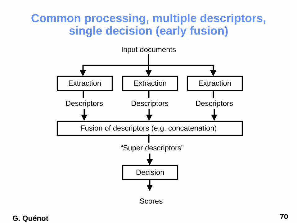
Common processing, multiple descriptors, single decision (early fusion)

Descriptors

Input documents

Decision

Extraction

Scores

Descriptors

Extraction

Descriptors

Extraction

Fusion of descriptors (e.g. concatenation)

“Super descriptors”

G. Quénot 71

Common processing, multiple descriptors, multiple decision (late fusion)

Descriptors

Input documents

Decision

Extraction

Scores

Descriptors

Extraction

Descriptors

Extraction

Fusion of scores (e.g. arithmetic mean)

“Consolidated scores”

Decision

Scores

Decision

Scores

G. Quénot 72

Fusion of representations (early)

• For all vector description (of fixed size), whatever their origin,

• Possibility to concatenate the various descriptors in a unique mixed descriptor → normalization problem,

• Possibility to reduce la dimension of the resulting vector (and/or of each original vector) in order to keep only the most relevant information:

– Principal Component Analysis,– Neural networks,– Learning is needed (representative data and process).

• Less information, faster once learning is done,• Euclidean distance on the shortened vector.

G. Quénot 73

Fusion of the correspondence functions (late)

• Each correspondence function generally produces a quantitative value that estimate a similarity,

• It is always possible to come to the case in which the values are between 0 and 1 and represent a relevance,

• In order to fuse the results from several functions, we may use :

– A weighted sum,– A weighted product (weighted sum on the ogarithms),– The minimum value,– A classifier (SVM, neural network, …)

• Problem for the choice of the weights and/or for the classifier training.

G. Quénot 74

Computation of the relevance• Euclidean distance, angle between vectors,• Comparison between a query vector to all the

vectors in the database (no pre-selection),• “Small” number of dimensions ( < 10) : clustering

techniques hierarchical search,• “Medium” number of dimensions ( ~ 10+) :

methods based on space partitioning,• “Large” number of dimensions( >> 10 ) : no known

method faster that a full linear scan,• Reduction of the number of dimensions by

Principal Component Analysis.

G. Quénot 75

Principal Component Analysis 1• “Natural” data contain redundancies:

– Neighbor pixels’ values are correlated– Political opinions and age of people are correlated– Weight and size of objects are correlated– …

• Principal Component Analysis aims at– Identify and characterize redundancies in data– Transform data for removing and reducing

redundancies and possibly noise– “Ordinary or classical” PCA operates in the context of

linear algebra (non linear variants also exist)

G. Quénot 76

Principal Component Analysis 2

• Redundancies are identified as correlations• Correlation is measured by covariance

– Considering a set of samples 𝑥𝑥𝑖𝑖 ,𝑦𝑦𝑖𝑖 , 𝑖𝑖 ∈ 1 …𝑁𝑁 , covariance is defined as:

with:

– Correlation is defined as:

𝐜𝐜𝐜𝐜𝐜𝐜 𝒙𝒙,𝒚𝒚 =𝟏𝟏𝑵𝑵�𝒊𝒊=𝟏𝟏

𝒊𝒊=𝑵𝑵

𝑥𝑥𝑖𝑖 − �𝒙𝒙 𝑦𝑦𝑖𝑖 − �𝒚𝒚 �𝒙𝒙 =𝟏𝟏𝑵𝑵�𝒊𝒊=𝟏𝟏

𝒊𝒊=𝑵𝑵

𝑥𝑥𝑖𝑖

𝐫𝐫 =𝐜𝐜𝐜𝐜𝐜𝐜 𝒙𝒙,𝒚𝒚

𝐜𝐜𝐜𝐜𝐜𝐜 𝒙𝒙,𝒙𝒙 𝐜𝐜𝐜𝐜𝐜𝐜 𝒚𝒚,𝒚𝒚

G. Quénot 77


• Examples: no correlation (normal distributions)

cov(x,x) = 2500 cov(x,x) = 2500 cov(x,x) = 625cov(x,y) = 0 cov(x,y) = 0 cov(x,y) = 0cov(y,y) = 2500 cov(y,y) = 225 cov(y,y) = 2500r = 0 r = 0 r = 0

G. Quénot 78


• Examples: correlation (normal distributions)

cov(x,x) = 1800 cov(x,x) = 1800 cov(x,x) = 2500cov(x,y) = 1350 cov(x,y) = −1350 cov(x,y) = 1470cov(y,y) = 1800 cov(y,y) = 1800 cov(y,y) = 900r = +0.75 r = −0.75 r = 0.98

G. Quénot 79

Principal Component Analysis 5• Covariance matrix:

Σ = 𝐜𝐜𝐜𝐜𝐜𝐜(𝒙𝒙,𝒙𝒙) 𝐜𝐜𝐜𝐜𝐜𝐜(𝒙𝒙,𝒚𝒚)𝐜𝐜𝐜𝐜𝐜𝐜(𝒚𝒚,𝒙𝒙) 𝐜𝐜𝐜𝐜𝐜𝐜(𝒚𝒚,𝒚𝒚)

• Properties:– Σ is symmetric and positive → diagonalizable– ∃ rotation matrix R so that R−1ΣR is diagonal– If the rotation R is applied to the data:

• Σ becomes diagonal• r becomes 0• the x and y components becomes decorrelated• redundancy is removed• Independent components can be sorted according to their

variance (square root of the diagonal term)

G. Quénot 80


• Rotation (and translation) of the data

cov(x,x) = 2500 cov(x,x) = 3364cov(x,y) = 1470 cov(x,y) = 0cov(y,y) = 900 cov(y,y) = 49r = 0.98 r = 0

G. Quénot 81

Principal Component Analysis 7• Generalization from sets of two-dimensional

samples 𝑥𝑥𝑖𝑖 ,𝑦𝑦𝑖𝑖 , 𝑖𝑖 ∈ 1 …𝑁𝑁to sets of D-dimensional samples𝑥𝑥𝑖𝑖1, 𝑥𝑥𝑖𝑖2 … 𝑥𝑥𝑖𝑖𝐷𝐷 , 𝑖𝑖 ∈ 1 …𝑁𝑁

• Σ is a D×D symmetric and positive matrix that can be diagonalized as R−1ΣR

• Data can be rotated and centered accordingly into decorrelated components of decreasing variance

Σ𝒋𝒋𝒋𝒋 = 𝐜𝐜𝐜𝐜𝐜𝐜 𝒙𝒙.𝒋𝒋,𝒙𝒙.𝒋𝒋 =𝟏𝟏𝑵𝑵�𝒊𝒊=𝟏𝟏

𝒊𝒊=𝑵𝑵

𝑥𝑥𝑖𝑖𝑗𝑗 − 𝒙𝒙.𝒋𝒋 𝑥𝑥𝑖𝑖𝑘𝑘 − 𝒙𝒙.𝒋𝒋

G. Quénot 82

Principal Component Analysis 8• With real high-dimensional sets of samples, the

variance of the decorrelated components decreases very rapidly

• If correlation is high in the data, many of the last components have very small variances

• Dropping the components with very small variance does not significantly change the results

• Dropping components whose variance is smaller than the level of noise even improve performance

• Dropping components is a linear projection

G. Quénot 83

Principal Component Analysis 9• PCA summary:

– Translation to center of data (removing mean vector)– Rotation to the principal axes (from covariance matrix)– Projection on the “big variance” axes (dropping of small

variance components)• PCA (almost) preserve the Euclidean distance

– Translation and rotation are isometries: they preserve Euclidean distance

– Projection dropping only small variance axes is close to an isometry: Euclidean distance is almost preserved

• Real data do not follow normal distributions but do exhibit significant correlations anyway

G. Quénot 84

User interface• Classical interface for the part of the query given at the

semantic level (e.g. text input for keywords),• Plus possibility to define a query at the signal level:

– Query by example : one or several images or video segments, initially given or selected during relevance feedback,

– Library of signal elements : colors, textures,shapes (that could be entered as sketches),

– Possibility to define a relative importance for the various signal (or semantic) features available,

– Possibility to define a fusion method for the correspondence functions (sum, product, min, …),

– The system can also mek these choices by analysis of the relevance feedback,

– Link between signal and semantics.

G. Quénot 85

MPEG-7

• “Multimedia Content Description Interface”• All levels, all application, all domains, ....

G. Quénot 86

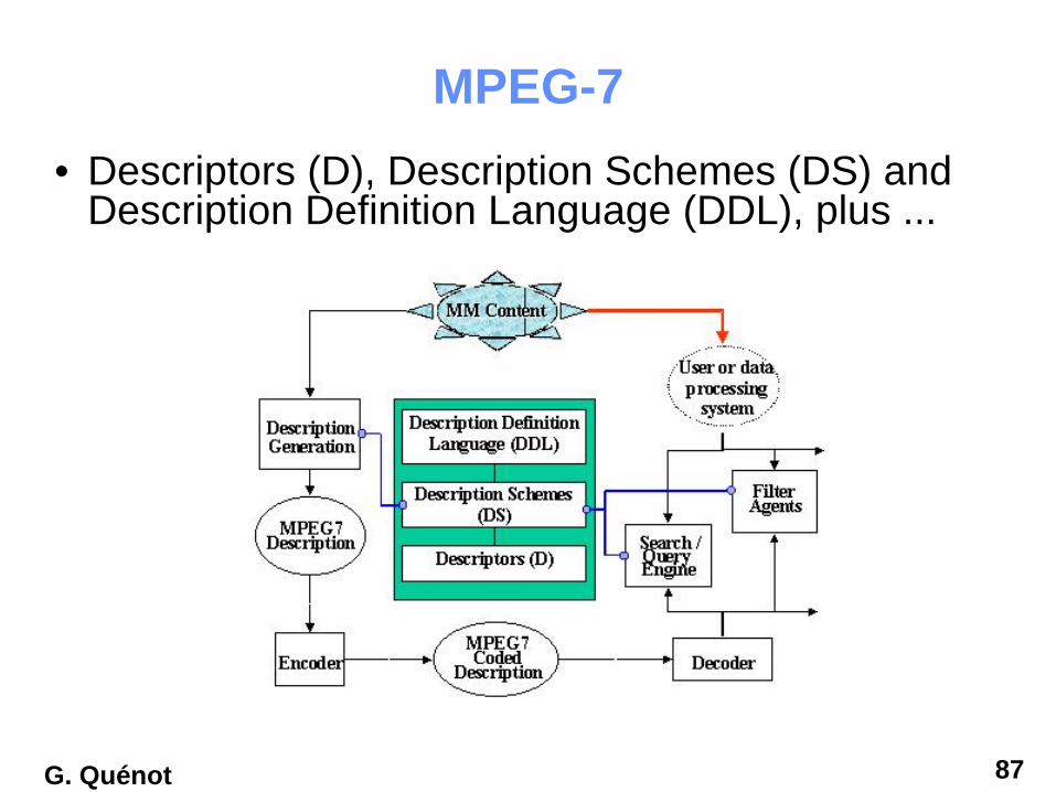
MPEG-7• Descriptors (D), Description Schemes (DS) and

Description Definition Language (DDL), plus ...

G. Quénot 87

MPEG-7• Descriptors (D), Description Schemes (DS) and

Description Definition Language (DDL), plus ...

G. Quénot 88

MPEG-7 parts1. MPEG-7 Systems - the tools that are needed to prepare MPEG-7

Descriptions for efficient transport and storage, and to allow synchronization between content en descriptions. Tools related to managing and protecting intellectual property

2. MPEG-7 Description Definition Language - the language for defining new Description Schemes and perhaps eventually also for new Descriptors.

3. MPEG-7 Audio – the Descriptors and Description Schemes dealing with (only) Audio descriptions

4. MPEG-7 Visual – the Descriptors and Description Schemes dealing with (only) Visual descriptions

5. MPEG-7 Multimedia Description Schemes - the Descriptors and Description Schemes dealing with generic features and multimedia descriptions

6. MPEG-7 Reference Software - a software implementation of relevant parts of the MPEG-7 Standard

7. MPEG-7 Conformance - guidelines and procedures for testing conformance of MPEG-7 implementations.

G. Quénot 89

MPEG-7 Systems

• Tools that are needed to prepare MPEG-7 Descriptions for efficient transport and storage, and to allow synchronization between content and descriptions

• Tools related to managing and protecting intellectual property.

• Defines the terminal architecture and the normative interfaces

G. Quénot 90

MPEG-7 Description Definition Language

• “... a language that allows the creation of new Description Schemes and, possibly, Descriptors. It also allows the extension and modification of existing Description Schemes.”

• XML Schema Language has been selected to provide the basis for the DDL. As a consequence of this decision, the DDL can be broken down into the following logical normative components:• The XML Schema structural language components;• The XML Schema data type language components;• The MPEG-7 specific extensions.

G. Quénot 91

MPEG-7 Audio

• Audio description framework (which includes the scale tree and low-level descriptors),

• Sound effect description tools,• Instrumental timbre description tools,• Spoken content description,• Uniform silence segment,• Melodic descriptors to facilitate query-by-

humming

G. Quénot 92

MPEG-7 Visual

• Color• Texture • Shape• Motion• Localization• Others

G. Quénot 93

MPEG-7 / Dublin Core Index StructureImpossible d’afficher l’image.

G. Quénot 94

Search at the signal level: conclusion

• Representation by different types of descriptors and evaluation of relevance by various functions,

• A single type: results from poor to average,• Several types simultaneously: results from

average to good with possible domain adaptation• Possibility to adjust the compromise quality -

performance - general - size of the database• Performance limited by the "analog" (not symbolic)

aspect of representations.