1

Integer-to-Integer Transform

整 數 轉 換

Speaker: 丁 建 均

國立台灣大學電信工程學研究所

2

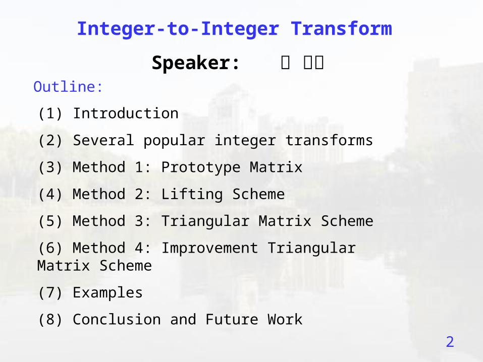
Integer-to-Integer Transform

Outline:

(1) Introduction

(2) Several popular integer transforms

(3) Method 1: Prototype Matrix

(4) Method 2: Lifting Scheme

(5) Method 3: Triangular Matrix Scheme

(6) Method 4: Improvement Triangular Matrix Scheme

(7) Examples

(8) Conclusion and Future Work

Speaker: 丁 建均

3

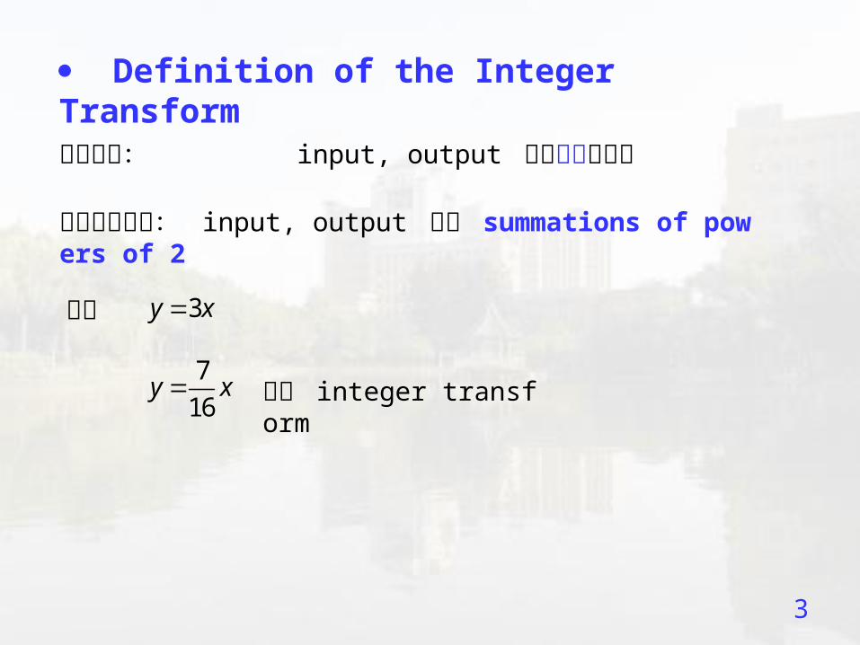
Definition of the Integer Transform

原始定義： input, output 皆為整數的運算

修正後的定義： input, output 皆為 summations of powers of 2

例如 3y x

7

16y x 皆為 integer transform

4

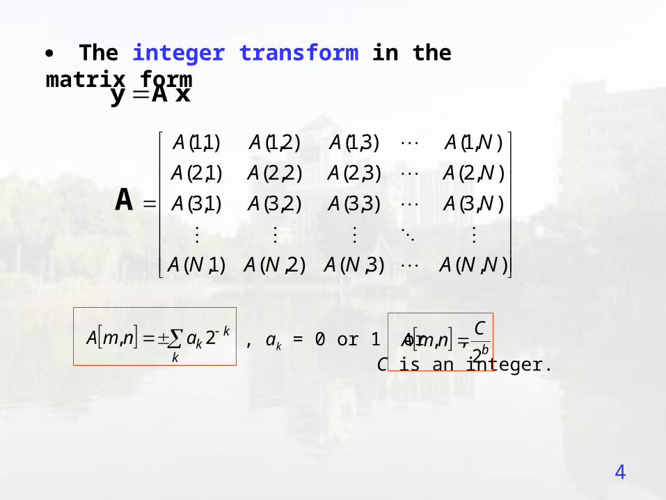
The integer transform in the matrix form

y A x

(1,1) (1,2) (1,3) (1, )

(2,1) (2,2) (2,3) (2, )

(3,1) (3,2) (3,3) (3, )

( ,1) ( ,2) ( ,3) ( , )

A A A A N

A A A A N

A A A A N

A N A N A N A N N

A

, ak = 0 or 1 or , C is an integer. k

kkanmA 2,

b

CnmA

2,

5

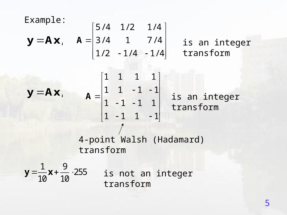
Example: 5 / 4 1/ 2 1/ 4

3 / 4 1 7 / 4

1/ 2 1/ 4 1/ 4

A is an integer transform

1 1 1 1

1 1 1 1

1 1 1 1

1 1 1 1

A is an integer transform

1 9255

10 10 y x is not an integer transform

,y Ax

,y Ax

4-point Walsh (Hadamard) transform

6

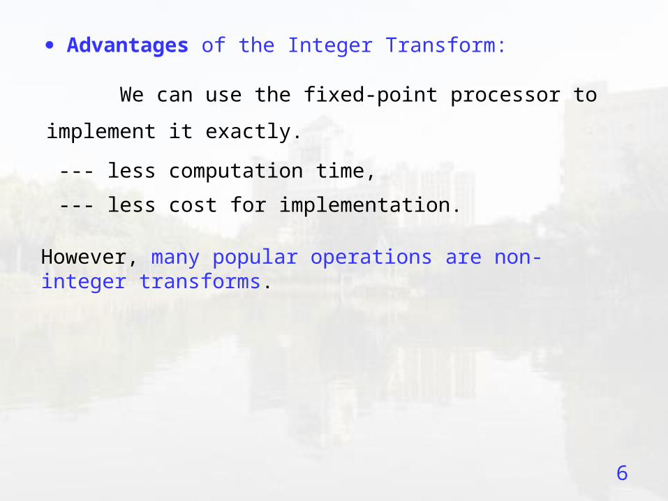
Advantages of the Integer Transform:

We can use the fixed-point processor to implement it exactly.

--- less computation time,

--- less cost for implementation.

However, many popular operations are non-integer transforms.

7

Discrete Fourier transform:

2[ , ] expA m n j mn

N

Discrete cosine transform:

2[ , ] cosmA m n k mn

N

RGB to YCbCr Transform

0.299 0.587 0.114

0.5 0.419 0.081

0.169 0.331 0.5

A

Karhunen-Loeve transform

Wavelet transform

8

How do we convert a non-integer transform into an integer transform?

9

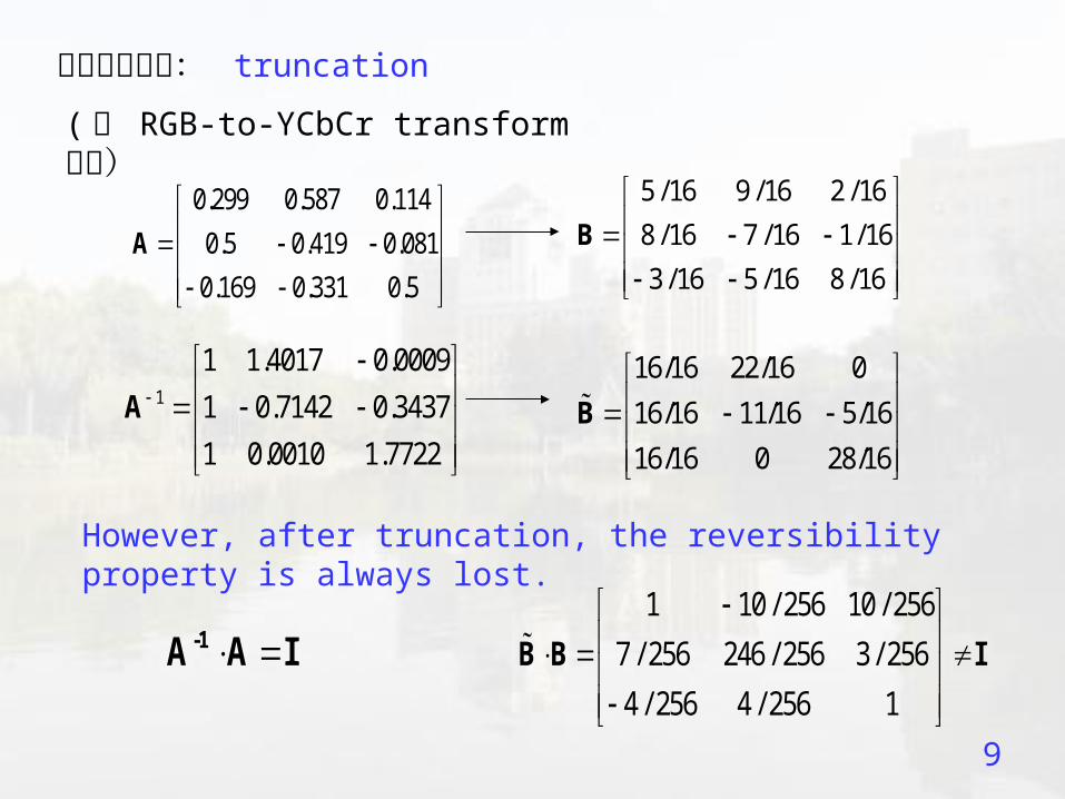
最簡單的方法： truncation

0.299 0.587 0.114

0.5 0.419 0.081

0.169 0.331 0.5

A

5 /16 9 /16 2 /16

8 /16 7 /16 1/16

3 /16 5 /16 8 /16

B

1

1 1.4017 0.0009

1 0.7142 0.3437

1 0.0010 1.7722

A16/16 22/16 0

16/16 11/16 5/16

16/16 0 28/16

B

1 10 / 256 10 / 256

7 / 256 246 / 256 3 / 256

4 / 256 4 / 256 1

B B I -1A A I

However, after truncation, the reversibility property is always lost.

( 以 RGB-to-YCbCr transform 為例）

10

In JPEG 2000 standard, the RGB-to-YCbCr transform is approximated as follows:

0.299 0.587 0.114

0.5 0.419 0.081

0.169 0.331 0.5

A

0.25 0.5 0.25

1 1 0

0 1 1

B

1

1 1.4017 0.0009

1 0.7142 0.3437

1 0.0010 1.7722

A

1 0.75 0.25

1 0.25 0.25

1 0.25 0.75

B

B B I is satisfied

11

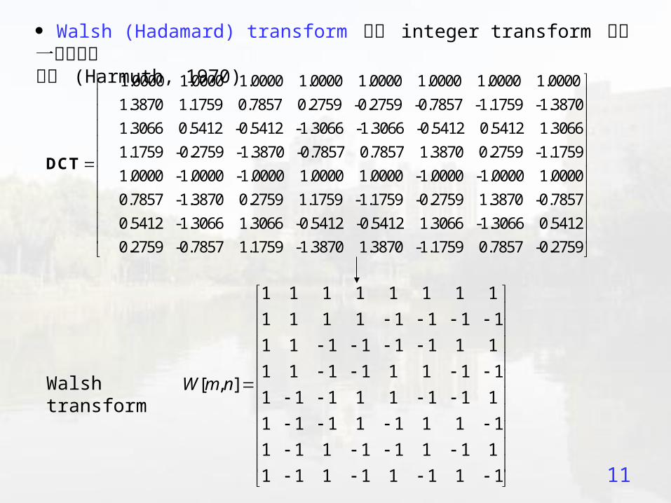
Walsh (Hadamard) transform 也是 integer transform 當中一個重要的例子 (Harmuth, 1970)

1 1 1 1 1 1 1 1

1 1 1 1 1 1 1 1

1 1 1 1 1 1 1 1

1 1 1 1 1 1 1 1[ , ]

1 1 1 1 1 1 1 1

1 1 1 1 1 1 1 1

1 1 1 1 1 1 1 1

1 1 1 1 1 1 1 1

W m n

1.0000 1.0000 1.0000 1.0000 1.0000 1.0000 1.0000 1.0000

1.3870 1.1759 0.7857 0.2759 -0.2759 -0.7857 -1.1759 -1.3870

1.3066 0.5412 -0.5412 -1.30

DCT

66 -1.3066 -0.5412 0.5412 1.3066

1.1759 -0.2759 -1.3870 -0.7857 0.7857 1.3870 0.2759 -1.1759

1.0000 -1.0000 -1.0000 1.0000 1.0000 -1.0000 -1.0000 1.0000

0.7857 -1.3870 0.2759 1.1759 -1.1759 -0.2759 1.3870 -0.7857

0.5412 -1.3066 1.3066 -0.5412 -0.5412 1.3066 -1.3066 0.5412

0.2759 -0.7857 1.1759 -1.3870 1.3870 -1.1759 0.7857 -0.2759

Walsh transform

12

In Ohta’s work in 1980

0.515619 0.565412 0.543575

0.754932 0.181361 0.527458

0.212700 0.726941 0.554383

A

0.25 0.5 0.25

0.5 0 0.5

0.25 0.5 0.25

B

(KLA transform, one of the color transform)1

1 1 1

1 0 1

1 1 1

B

In MPEG-40.5 0.5 0.5 0.5

0.6533 0.2706 0.2706 0.6533

0.5 0.5 0.5 0.5

0.2706 0.6533 0.6533 0.2706

C

(4-point DCT)

1 1 1 1

2 1 1 2

1 1 1 1

1 2 2 1

B

13

Question:

How to convert other non-integer transforms into the integer transforms that satisfy the following requirements:

(2) Reversibility

(1) Integerization ,2

kk

bB m n

,

2kk

bB m n

B B I

(3) Accuracy B A, B" A-1 (or B A, B" -1A-1)

A, A-1: original non-integer transform pair,

B, B ̃: integer transform pair (4) Bit Constraint: The denominator ( 分母） 2k should not be too large.

(5) Less Complexity

14

Development of Integer Transforms:

(A) Prototype Matrix Method

(suitable for 2, 4, 8 and 16-point DCT, DST, DFT)

(B) Lifting Scheme

(suitable for 2k-point DCT, DST, DFT)

(C) Triangular Matrix Scheme

(suitable for any matrices, satisfies Goals 1 and 2)

(D) Improved Triangular Matrix Scheme

(suitable for any matrices, satisfies Goals 1 ~ 5)

15

Method 1: Prototype Matrix ( 模型矩陣）

基本精神：原來的 transform 長什麼樣子， integer transform 的「模型」就長什麼樣子

W. K. Cham, “Development of integer cosine transform by the principles of dynamic symmetry”, Proc. Inst. Elect. Eng., pt. 1, vol. 136, no. 4, pp. 276-282, Aug. 1989.

S. C. Pei and J. J. Ding, “The integer Transforms analogous to discrete trigonometric transforms,” IEEE Trans. Signal Processing, vol. 48, no. 12, pp. 3345-3364, Dec. 2000.

16

0.7010 0.7010 0.7010 0.7010 0.7010 0.7010 0.7010 0.7010

0.9808 0.8315 0.5556 0.1951 0.1951 0.5556 0.8315 0.9808

0.9239 0.3827 0.3827 0.9239 0.9239 0.3827 0.3827 0.9239

0.8315 0.1951 0.9808 0.5556 0.5556 0.9808 0.1951 0.

8315

0.7010 0.7010 0.7010 0.7010 0.7010 0.7010 0.7010 0.7010

0.5556 0.9808 0.1951 0.8315 0.8315 0.1951 0.9808 0.5556

0.3827 0.9239 0.9239 0.3827 0.3827 0.9239 0.9239 0.3827

0.1951 0.5556 0.8315 0.9808 0.9808 0.8315 0

.5556 0.1951

1 2 3 4 4 3 2 1

1 2 2 1 1 2 2 1

2 4 1 3 3 1 4 2

3 1 4 2 2 4 1 3

2 1 1 2 2 1 1 2

4 3 2 1 1 2 3 4

1 1 1 1 1 1 1 1

1 1 1 1 1 1 1 1

a a a a a a a a

b b b b b b b b

a a a a a a a a

a a a a a a a a

b b b b b b b b

a a a a a a a a

B

0.9808 a1, 0.8315 a2, 0.5556 a3, 0.1951 a4, 0.9239 b1, 0.3827 b1.

8-Point DCT

6 parameters

17

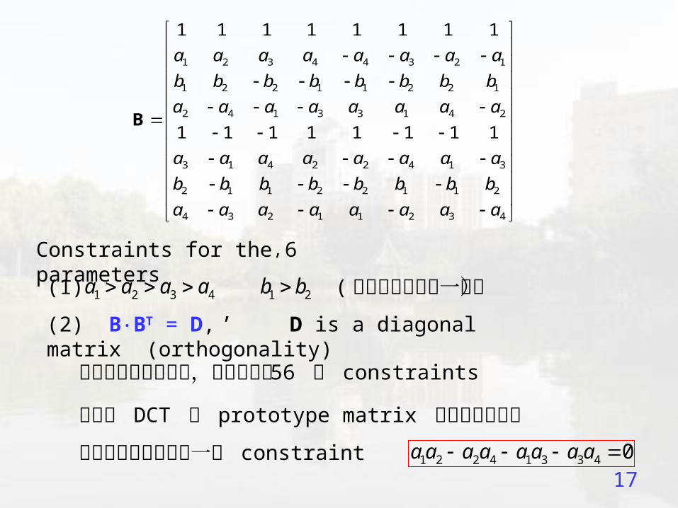
Constraints for the 6 parameters

1 2 3 4 4 3 2 1

1 2 2 1 1 2 2 1

2 4 1 3 3 1 4 2

3 1 4 2 2 4 1 3

2 1 1 2 2 1 1 2

4 3 2 1 1 2 3 4

1 1 1 1 1 1 1 1

1 1 1 1 1 1 1 1

a a a a a a a a

b b b b b b b b

a a a a a a a a

a a a a a a a a

b b b b b b b b

a a a a a a a a

B

(1) , 1 2 3 4a a a a 1 2b b

,

(2) BBT = D, D is a diagonal matrix (orthogonality)

( 大小順序和原來一樣）

這個式子看起來簡單，但是其實有 56 個 constraints但由於 DCT 的 prototype matrix 有特殊的對稱性

所以可以簡化成只有一個 constraint 1 2 2 4 1 3 3 4 0a a a a a a a a

18

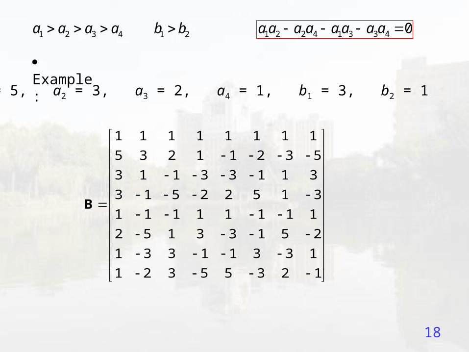
1 2 3 4a a a a 1 2b b 1 2 2 4 1 3 3 4 0a a a a a a a a

Example:

a1 = 5, a2 = 3, a3 = 2, a4 = 1, b1 = 3, b2 = 1

1 1 1 1 1 1 1 1

5 3 2 1 1 2 3 5

3 1 1 3 3 1 1 3

3 1 5 2 2 5 1 3

1 1 1 1 1 1 1 1

2 5 1 3 3 1 5 2

1 3 3 1 1 3 3 1

1 2 3 5 5 3 2 1

B

19

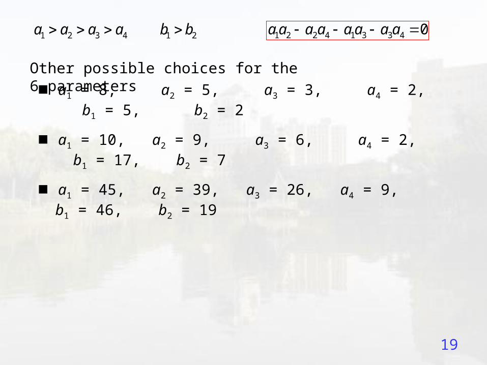
Other possible choices for the 6 parameters

1 2 3 4a a a a 1 2b b 1 2 2 4 1 3 3 4 0a a a a a a a a

a1 = 8, a2 = 5, a3 = 3, a4 = 2, b1 = 5, b2 = 2

a1 = 10, a2 = 9, a3 = 6, a4 = 2, b1 = 17, b2 = 7

a1 = 45, a2 = 39, a3 = 26, a4 = 9, b1 = 46, b2 = 19

20

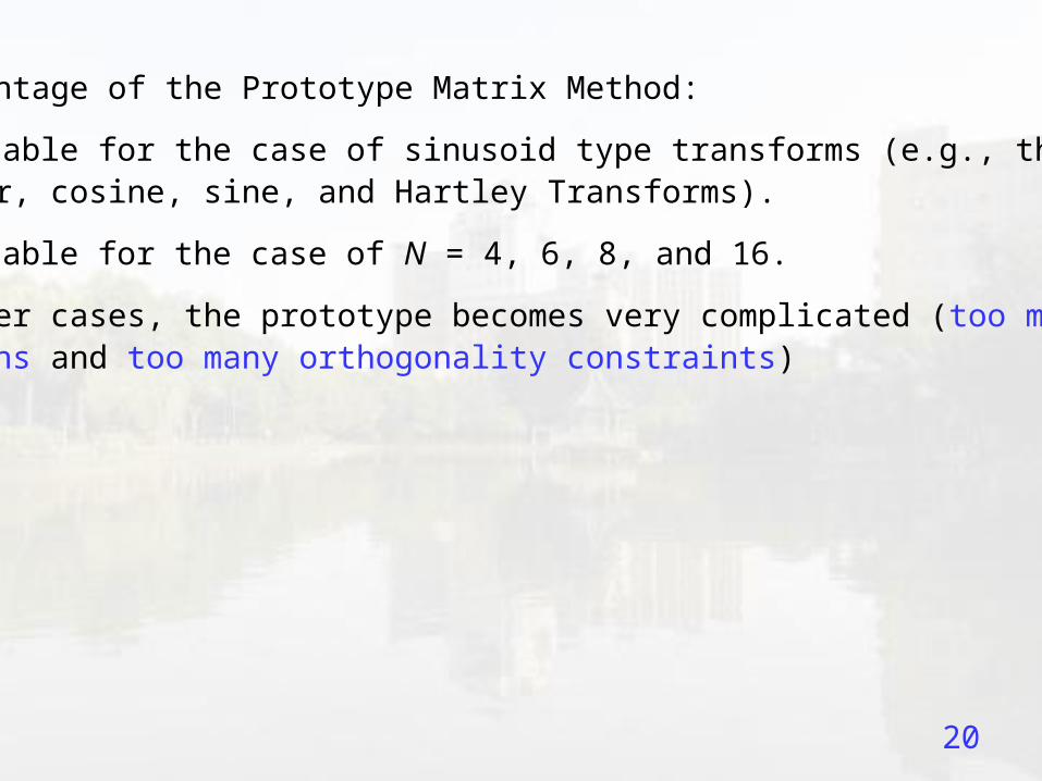
--- Disadvantage of the Prototype Matrix Method:

Only suitable for the case of sinusoid type transforms (e.g., the discrete Fourier, cosine, sine, and Hartley Transforms).

Only suitable for the case of N = 4, 6, 8, and 16.

In other cases, the prototype becomes very complicated (too many unknowns and too many orthogonality constraints)

21

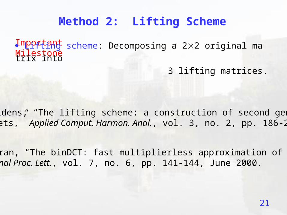
Method 2: Lifting Scheme

Important Milestone

Lifting scheme: Decomposing a 22 original matrix into

3 lifting matrices.

W. Sweldens, “The lifting scheme: a construction of second generation wavelets,” Applied Comput. Harmon. Anal., vol. 3, no. 2, pp. 186-200, 1996.

T. D. Tran, “The binDCT: fast multiplierless approximation of the DCT,” IEEE Signal Proc. Lett., vol. 7, no. 6, pp. 141-144, June 2000.

22

1 ( 1) / 1 0 1 ( 1) /

0 1 1 0 1

a b a c d c

c d c

A

1 0 1 1 0

( 1) / 1 0 1 ( 1) / 1

a b b

c d d b a b

A

Decomposing a 2 2 matrix:

or

Constraint: det(B) = ad bc = 1.

a

b

c

d

(a-1)/c (d-1)/c c

23

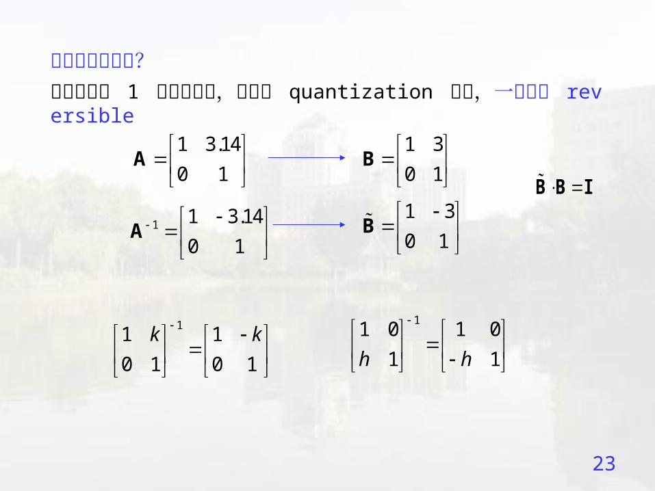
為什麼要這麼做？因為對角為 1 的三角矩陣，在經過 quantization 之後，一定還是 reversible

1 3.14

0 1

A

1 1 3.14

0 1

A

1 3

0 1

B

1 3

0 1

B

B B I

11 1

0 1 0 1

k k

11 0 1 0

1 1h h

24

1 ( 1) / 1 0 1 ( 1) /

0 1 1 0 1

a c d c

c

A

approximation

31

2

1 3

2

1 01 / 2 1 / 2

/ 2 10 1 0 1

kk

k

B

3 1 2 31 2 1

2 32

3 1 2 31 2 1

2 32

12 2 2 2

12 2

k k k kk k k

k kk

where 11( 1) / / 2 ,ka c 2

2 / 2 ,kc 33( 1) / / 2 ,kd c

3 1

2

13

2

1 0 1 / 21 / 2

/ 2 1 0 10 1

k k

k

B

3 2 3 1 2 31

2 2 1

3 2 3 1 2 31

2 2 1

12 2 2 2

12 2

k k k k k kk

k k k

25

Extension to the 2k-point case

Many 2k-point discrete operations can be decomposed into (N/2)log2N butterflies

Example: 8-point discrete Fourier transform (DFT)

x[0]

x[4]

x[2]

x[6]

x[1]

x[5]

x[3]

x[7]

X[0]

X[1]

X[2]

X[3]

X[4]

X[5]

X[6]

X[7]

-1

-1

-1

-1

-1

-1

-1

-1

1

w2

1

w2

1

w

w2

w3

-1

-1

-1

-1

26

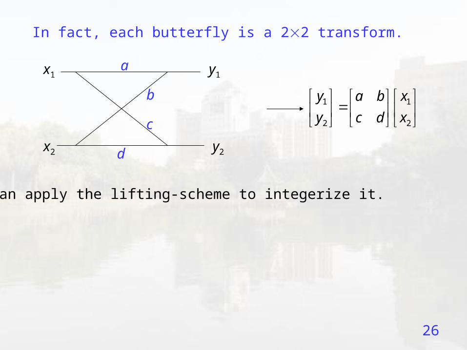
In fact, each butterfly is a 22 transform.

We can apply the lifting-scheme to integerize it.

1 1

2 2

y xa b

y xc d

x1

x2

y1

y2

a

b

c

d

27

Advantages:

--- Easy for design (avoiding solving the N(N 1) orthogonality constraint)

--- Flexibility: 1/2k1, 2/2k2, 3/2k3, are free to choose

--- The fast algorithm of the original non-integer transform can be preserved.

The 2k-point integer discrete Fourier, cosine, sine, Hartley, and Wavelet

transforms can hence be derived (k can be any integer).

S. Oraintara, Y. J. Chen, and T. Q. Nguyen, “Integer fast Fourier transform”, IEEE Trans. Signal Processing, vol. 50, no. 3, pp. 607-618, March 2002.

28

Method 3: Triangular Matrix Scheme

Lifting scheme: 2 2 matrix

Triangular matrix scheme: Generalizing the lifting scheme for N N matrices, where N can be any integer.

P. Hao and Q. Shi., “Matrix factorizations for reversible integer mapping”, IEEE Trans. Signal Processing, vol. 49, no. 10, pp. 2314-2324, Oct. 2001.

S. C. Pei and J. J. Ding, “Improved reversible integer transform”, ISCAS, pp. 1091-1094, May 2006.

29

Important discovery:

“All” the reversible non-integer transforms (det(A)) 0) can be c

onverted into the reversible integer transforms by the triangular m

atrix scheme.

30

Any matrix whose determinant is a power of 2 can be decomposed as follows:

A = DLUS

D: diagonal matrix L: lower triangular matrix,

U: upper triangular matrix, S: One row lower triangular matrix

N

N

k

k

k

ks

2000

0200

0020

0002

1

2

1

D

1

01

001

0001

00001

1,3,2,1,

3,12,11,1

2,31,3

1,2

NNNNN

NNN

cccc

ccc

cc

c

L

10000

1000

100

10

1

,1

,31,3

,21,23,2

,11,13,12,1

NN

NN

NN

NN

h

hh

hhh

hhhh

U

1

01000

00100

00010

00001

1321 Nssss

S

31

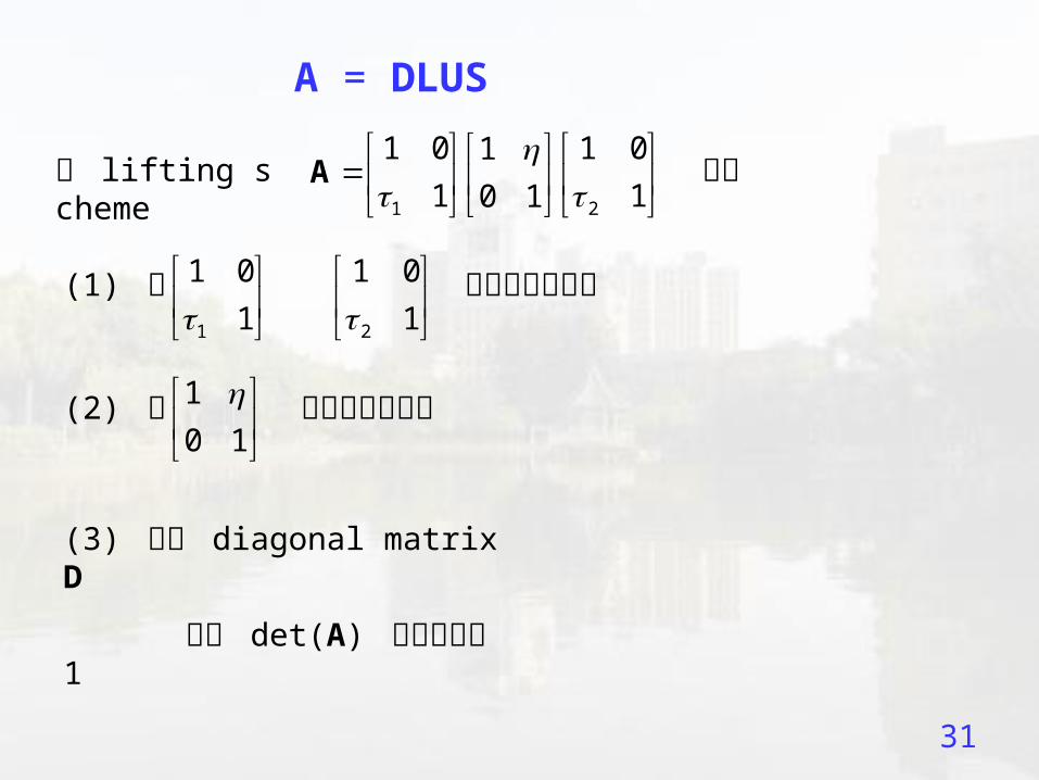
A = DLUS

1 2

1 0 1 01

1 10 1

A和 lifting schem

e比較

(1) 把1

1 0

1 2

1 0

1

變成下三角矩陣

(2) 把 1

0 1

變成上三角矩陣

(3) 多了 diagonal matrix D

使得 det(A) 不再限定為 1

32

Advantages of Triangular Matrix Decomposition:

-- The inverse of a triangular matrix is easy to compute.

-- The inverse of an integer triangular matrix is also an

integer triangular matrix.

11 0 0 1 0 0

2 1 0 2 1 0

3 4 1 5 4 1

11 -1/8 1/2 -1/2 1/2

0 1 11/8 17/8 1/2

0 0 1 2 7/8

0 0 0 1 -1/8

0 0 0 0 1

1 1/8 -43/64 101/64 57/256

0 1 -11/8 5/8 32/25

0 0 1 -2 -9/8

0 0 0 1 1/8

0 0 0 0 1

33

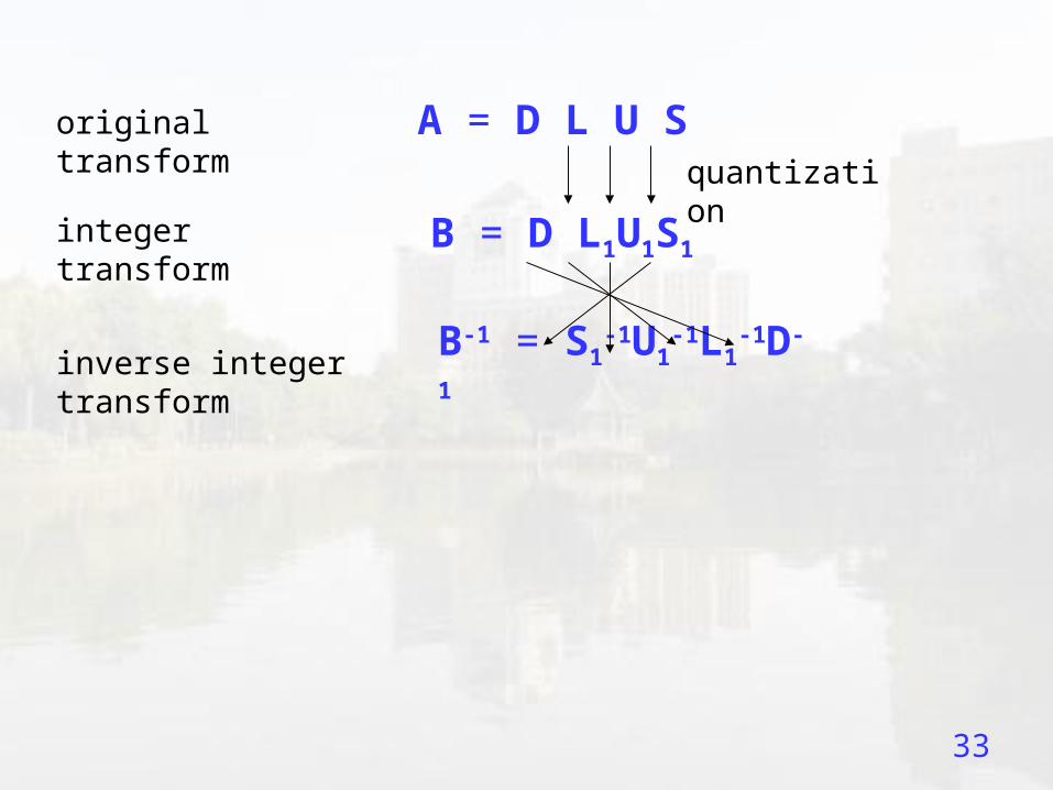
A = D L U Squantization

B = D L1U1S1

original transform

integer transform

inverse integer transform B-1 = S1-1U1

-1L1-1D-1

34

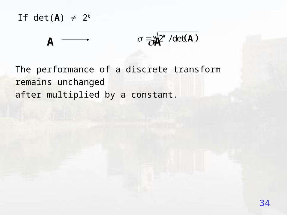
If det(A) 2k

A A 2 / detkN A

The performance of a discrete transform remains unchanged

after multiplied by a constant.

35

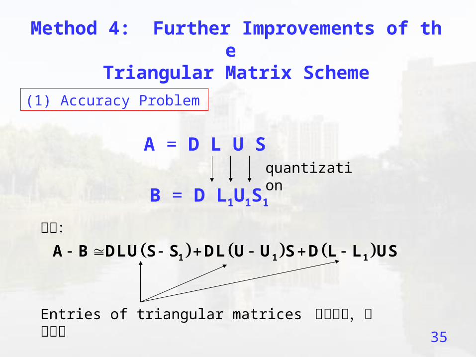
Method 4: Further Improvements of the Triangular Matrix Scheme

(1) Accuracy Problem

A = D L U Squantization

B = D L1U1S1

1 1 1A B DLU S S DL U U S D L L US

Entries of triangular matrices 的值越小，誤差越小

誤差：

36

Decompose PAQ instead of A

row permutationmatrix

column permutationmatrix

PAQ = D L U S

PBQ = D L1U1S1

B = PTD L1U1S1QT

Try to find P and Q to minimize the entries of L, U, and S

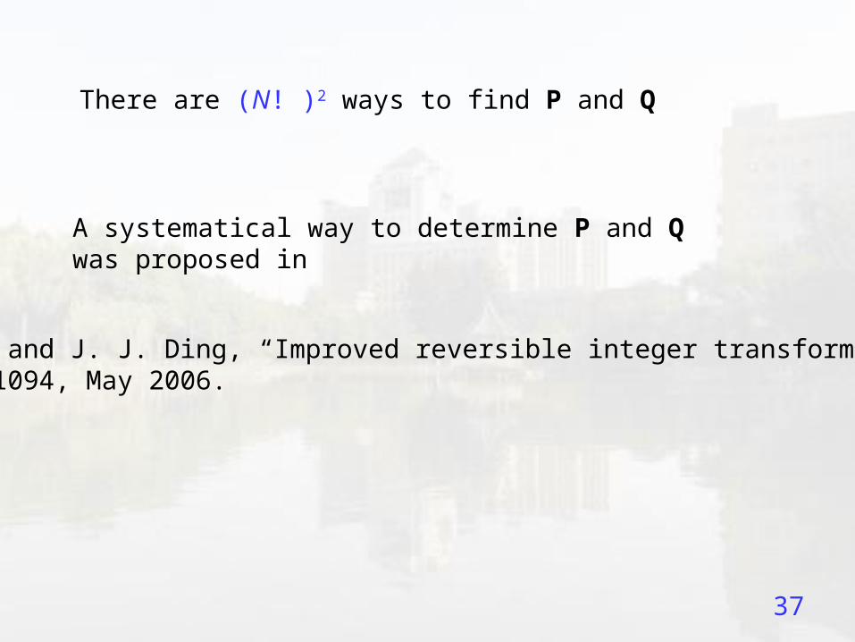
37

A systematical way to determine P and Q was proposed in

There are (N! )2 ways to find P and Q

S. C. Pei and J. J. Ding, “Improved reversible integer transform”, ISCAS, pp. 1091-1094, May 2006.

38

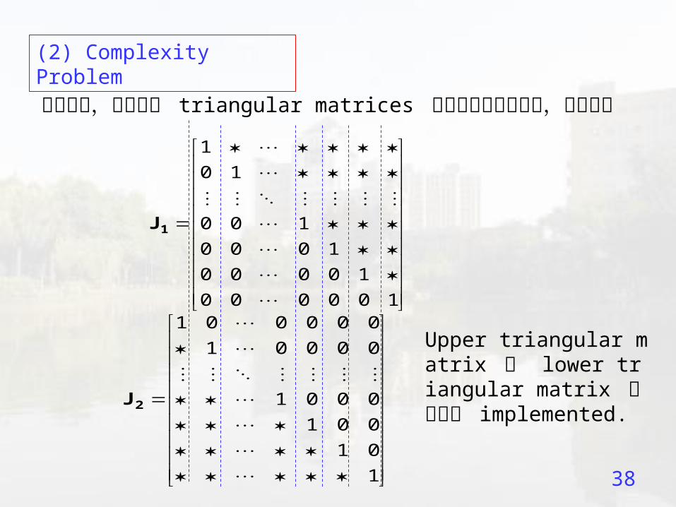
(2) Complexity Problem

乍看之下，變成三個 triangular matrices 好像會增加運算時間，其實不然

100000

10000

1000

100

10

1

1J

1

01

001

0001

00001

000001

2J

Upper triangular matrix 和　 lower triangular matrix 可以同時 implemented.

39

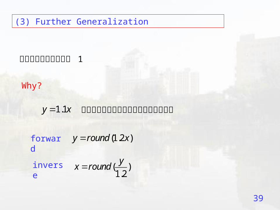
(3) Further Generalization

對角線其實不必都等於 1 　

Why?

1.1y x 這樣的運算其實可以變成可逆的整數轉換

forward (1.2 )y round x

inverse ( )1.2

yx round

40

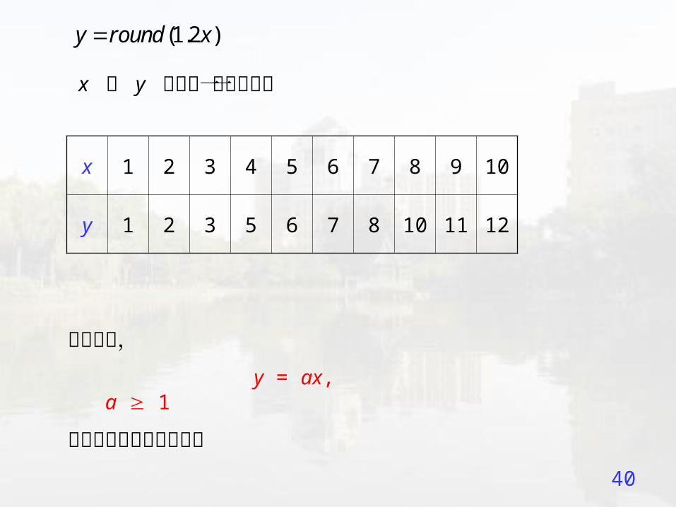
(1.2 )y round x

x 和 y 之間有一對一的關係

x 1 2 3 4 5 6 7 8 9 10

y 1 2 3 5 6 7 8 10 11 12

以此類推，

y = ax, a 1

必定也可以變成可逆轉換

41

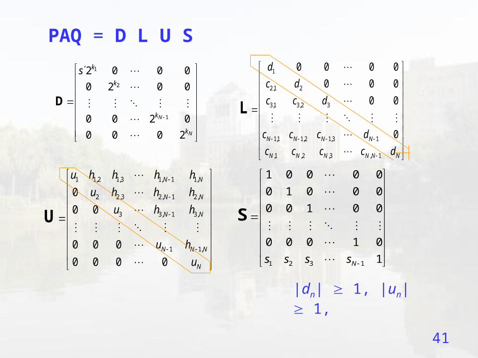
PAQ = D L U S

N

N

k

k

k

ks

2000

0200

0020

0002

1

2

1

D

1

2,1 2

3,1 3,2 3

1,1 1,2 1,3 1

,1 ,2 ,3 , 1

0 0 0 0

0 0 0

0 0

0N N N N

N N N N N N

d

c d

c c d

c c c d

c c c c d

L

1 1,2 1,3 1, 1 1,

2 2,3 2, 1 2,

3 3, 1 3,

1 1,

0

0 0

0 0 0

0 0 0 0

N N

N N

N N

N N N

N

u h h h h

u h h h

u h h

u h

u

U

1 2 3 1

1 0 0 0 0

0 1 0 0 0

0 0 1 0 0

0 0 0 1 0

1Ns s s s

S

|dn| 1, |un| 1,

42

這樣的方法，被稱作 scaled lifting scheme

或 scaled triangular matrix scheme

S. C. Pei and J. J. Ding, “Scaled lifting scheme and generalized reversible integer transform,” ISCAS, pp. 3203-3206, May 2007.

43

Examples

Integer Color Transform

RGB to YCbCr Transform

0.299 0.587 0.114

0.5 0.419 0.081

0.169 0.331 0.5

A

x1[1] = 4B, x1[2] = R, x1[3] = 2G,

1 1 2 1 11 1 { 346 [2] 339 [3]} / 256y x T x x

1 1 0 1 12 2 11 [1] 128 [3] / 256y x T y x

1 1 1 1 13 3 22 [1] 173 [2] / 256y x T y y

Y = y1[3]/2, Cr = y1[2], Cb = y1[1]/4.

2 2l lb l l

l l b

T a a

44

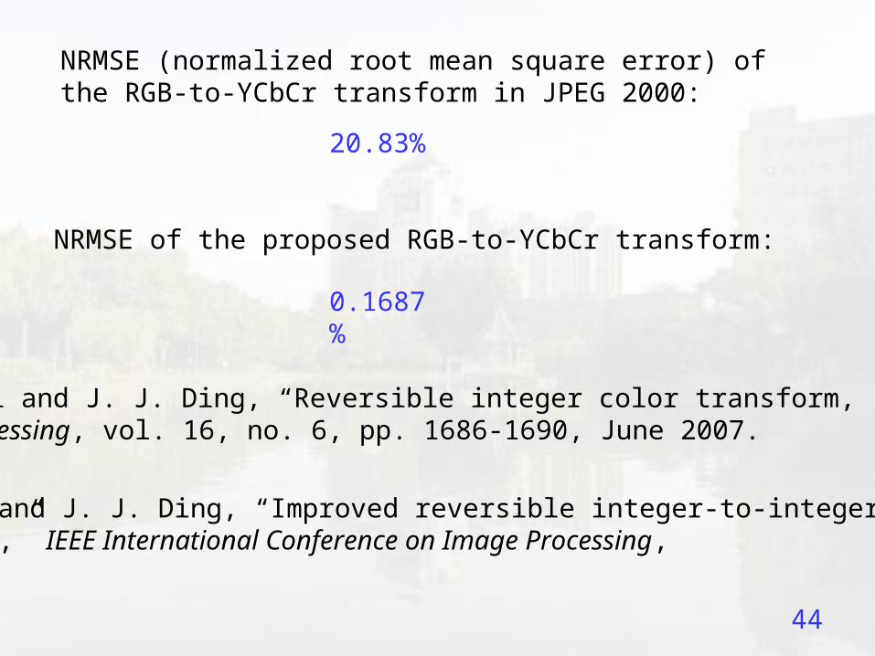
NRMSE (normalized root mean square error) of the RGB-to-YCbCr transform in JPEG 2000:

20.83%

NRMSE of the proposed RGB-to-YCbCr transform:

0.1687%

S. C. Pei and J. J. Ding, “Reversible integer color transform,” IEEE Trans. Image Processing, vol. 16, no. 6, pp. 1686-1690, June 2007.

S. C. Pei and J. J. Ding, “Improved reversible integer-to-integer color transforms,” IEEE International Conference on Image Processing, Nov. 2009.

45-100 -50 0 50 100

-5

0

5

10

15

-20 -10 0 10 20-5

0

5

10

15

-100 -80 -60 -40 -20 0 20 40 60 80 100-2

0

2

4

-100 -50 0 50 100-5

0

5

10

15

-20 -10 0 10 20-5

0

5

10

15By Origial 210-point DFT

By Integer DFT

x(t)

210-Point Integer Fourier Transform

46

Conclusion and Future Work The integer transform can apparently improve the efficiency of digital

signal processing and is important in VLSI design.

Future works:

(1) Faster design algorithm to find the optimal integer transform.

(2) Applied to the multi-channel filter system (Since it can be expressed by

a matrix)

(3) Pseudo-reversible integer transform (the case of det(A)=0)

http://djj.ee.ntu.edu.tw/Integer.ppt