1

Author version: Marine Ecology Progress Series: 389; 2009; 97-116 Hydrographic and Biological characteristics along 45°E longitude in the South Western Indian Ocean and Southern Ocean during austral summer 2004

P. Jasminea, K.R. Muraleedharana*, N.V. Madhu , C.R. Ashadevia, R. Alagarsamyb, C.T. Achuthankuttya, Zeena. P. Revia, V.N. Sanjeevanc, Satish sahayaka

a National Institute of Oceanography, Regional Centre, Dr. Salim Ali Road, P.B. No. 1918, Kochi-682 018, India b National Institute of Oceanography, Dona-Paula, Goa – 403 004, India c Center For Marine Living Resources and Ecology, Ministry of Earth Sciences, Kendriya Bhavan, P.B. No. 5415, Kochi, CSEZ P.O, Kakkanad – 37, India

Abstract

During the austral summer 2004, an intensive multidisciplinary survey was carried out in the Indian Ocean sector of the Southern Ocean to study the main hydrographic features and the associated productivity processes. This sector includes circumpolar zones and fronts with distinct hydrographic and trophic regimes, such as the Subtropical Zone, Subtropical Frontal Zone, Sub Antarctic Zone, Polar Frontal Zone, Northern Subtropical Front , Agulhas Retroflection Front, Southern Subtropical Front, Subantarctic Front, Surface Polar Front, and SubSurface Polar Front. Seasonal variations in the solar irradiance and day length, stratification, lack of micronutrients like iron and increased grazing pressure are the major factors that influenced or constrained biological production in this region. Even though there are broad differences in these controlling factors in time and space between the zonal regions, the upper 1000 m of the water column of the main zones viz. (STZ, STFZ, SAZ, PFZ) supported almost identical standing stocks of mesozooplankton (0.43, 0.47, 0.45 and 0.49 ml m-3, respectively) during the austral summer. This unexpected similarity can be explained either through the functioning of the microbial loop within STZ,STFZ and SAZ or the multivorous foodweb ecology within the PFZ. Dominance of ciliates in the microzooplankton community may be one facor resulting in the maintenance of a high mesozooplankton standing stock in SAZ. In contrast to the zones, frontal regions showed wide differences in hydrography and biological characteristics. The SSTF and SPF were far more biologically productive than that of NSTF and ARF.

Keywords: Fronts, Zones, Microzooplankton, Mesozooplankton, Microbial loop, Southern Ocean

* Corresponding author: Tel: +91 484 2390814 Fax: +91 484 2390618 E-Mail address : muraleedharan@nio.org

Present address : National Institute of Oceanography, Regional centre, Kochi, India

2

1. Introduction

The Southern Ocean (SO) plays a major role in regulating the global carbon fluxes and

world climate. Tropical regions are characterised by receiving a surplus solar energy whereas the

polar regions are in deficit of this not only during winter with either long or continuous nights,

but also during summer because of the sun’s low angle of incidence. Both atmospheric and

oceanic circulations regulate the global carbon budget by exporting the surplus energy from

tropical to Polar Regions. Fronts and the water masses of SO have great influence in regulating

biological production at the global scale (Abrams 1985a). Huntley et al. (1990) have reported

that the air breathing seabirds and mammals may transfer 20-25% of photosynthetically fixed

carbon into the atmosphere via respiration by consuming macrozooplankton and micronekton.

Therefore, zooplankton occupies an important position in the SO carbon cycle.

The major current system in the Indian Ocean sector of SO is the Antarctic Circumpolar

Current (ACC). The principal mechanism determining the different properties within the zones

and along the frontal systems is the wind (westerlies) induced transport that drives the

uninterrupted eastward flowing ACC. Deacon (1933, 1937) was the first to outline the frontal

systems in the SO and suggested that they are circumpolar. The majority of the studies on the

Southern Indian fronts were carried out during 1980’s (Lutjeharms 1981, Deacon 1982, 1983,

Belkin & Gordon 1996, Holliday & Read 1998, Pakhomov et al. 2000, Pollard & Read 2001).

Along the 45°E the main features are (from north to south), the existence of North Subtropical

Front (NSTF), Agulhas Retroflection Front (ARF), South Subtropical Front (SSTF),

Subantarctic Front (SAF) and Polar Front (PF); the PF has both Surface Polar Front (SPF) and

Subsurface Polar Front (SSPF) expressions. These frontal systems subdivide the sector into

zones with different biogeochemical characteristics viz., Subtropical Zone (STZ), Subtropical

Frontal Zone (STFZ), Subantarctic Zone (SAZ) and Polar Frontal Zone (PFZ) with Surface

Polar Zone (SPZ) and Subsurface Polar Zone (SSPZ) at 200 m. The Antarctic Paradox is related

to a well-known phenomenon referred to as the High Nutrient Low Chlorophyll (HNLC)

condition. i.e. There are regions where nitrogen and phosphorous are in high concentrations

throughout the year, but primary productivity is low. Subantarctic zone (SAZ) and Subantarctic

front (SAF) exhibit HNLC phenomenon prominently in the SO (El-Sayed 1984). The major

hypotheses put forward to explain the paradox are insufficient solar energy for phytoplankton

3

growth to attain its full potential (Nelson & Smith 1991), deficiency of micronutrients like iron

(Martin et al. 1990a & 1990), strong wind stirring resulting in deepening of the mixed layer

and convection (Sakshaug et al. 1991), and zooplankton grazing (Dubischar & Bathmann

1997).

The major currents that make this region so dynamic are the Agulhas and ACC. The

Agulhas Current (Gordon 1985) is the western boundary current that flows pole ward along the

east coast of Africa from 27° to ≈ 40°S, and then reverses direction or retroflects eastwards to

become the Agulhas Retroflection Current. The retroflection exhibits a quasi-stationary

meandering pattern with a wavelength of 500 km between 38° and 40°S (Gordon 1985). The

westerlies are largely confined between ~40° and ~65°S, and drive eastward surface current,

initiating a northward Ekman drift that is critical to the formation of Antarctic Intermediate

Water mass (AIW), subducted below the subantarctic surface water. The strong circumpolar

geostrophic currents and weak stratification result in the isopycnals tilting towards the surface in

the southern part of ACC. This tilting brings in deep water upwelling originating from the other

oceans and also from the deep Indian Ocean to the surface where they are modified by

atmospheric interactions. Another feature that results in the upwelling of nutrient-rich deep water

to the surface is the Antarctic Divergence (Jones et al. 1990). The upwelling deep water contains

not only high concentrations of dissolved nutrients that support rich biological productivity but

also supersaturated with carbon dioxide (CO2) that is vented to the atmosphere and plays a

substantial role in modulating atmospheric CO2 concentrations. The biological pump is another

mechanism whereby atmospheric CO2 concentrations can be drawn down and transferred into

the deep ocean. CO2 converted into organic matter by photosynthesis is exported to deeper

waters from the upper ocean by sedimentation and vertical migrations of organisms. The

westerlies have a large impact on SO hydrography, exerting a great influence both on the

distribution of sea ice and biological productivity. However, in oceanic waters beyond the

influence of landmasses, phytoplankton production of this region is consistently lower than

would normally be expected high macronutrient concentrations (Boyd et al. 2000).

The degree of variability in hydrographic and biological characteristics is high between

the zones and frontal system (Kostianoy et al. 2003 & 2004). Macro-scale zonation of the

epipelagic zooplankton in the SO has been extensively investigated (e.g. Grachev 1991,

4

Pakhomov &McQuaid 1996, Pakhomov et al. 2000). Although many studies have been

conducted in the Pacific and Atlantic sectors, the Indian Ocean sector still remains mostly

unexplored. A few studies in the Indian Ocean sector have focused in the vicinity of a major

front or zone (Bernard &Froneman 2003, Bernard & Froneman 2005, Froneman et al. 2007) and

the waters surrounding the oceanic islands (Fielding et al. 2007). However, an extensive study of

the response of biological community from the subtropical to polar region is still lacking. In

addition, whether HNLC affects the secondary productivity in the different zones has also not yet

been fully understood. The two major objectives of this study were, to describe the response of

biological community to different fronts and zones by switching to a food web structure better

adapted to the varying environment and to understand the influence of HNLC on the secondary

trophic level.

5

2. Data and Methodology

Hydrographic and biological measurements in the Indian Ocean sector of the SO were

carried out onboard FORV Sagar Kanya during the austral summer (January - February 2004).

Observations were made along 45°E, from 30°S to 55°S (Fig. 1), which passes through the major

fronts and zones between the subtropical and polar regions. Hydrographic observations were

taken at 1° latitudinal intervals, while the biological samples were collected at 2° intervals. A

SBE Seabird 911 plus CTD was used for recording temperature (accuracy ± 0.001°C) and

salinity (conductivity ± .0001 S/m) profiles up to 1000 m depth with a bin size of 1 m. Salinity

values from CTD were calibrated against the values obtained from water samples measured

using the Autosal (Guildline 8400A) onboard. The sea surface temperature (SST) was measured

using a bucket thermometer (accuracy of ± 0.2°C). AVHRR SST (spatial resolution 4 km and

temperature accuracy of about ± 0.3°C) were recorded over the time span of the cruise and

averaged for analysis. Surface meteorological parameters (air temperature, wind speed and

direction) were recorded at all stations. Plots of potential temperature versus salinity identified

the water masses and frontal structures. QuikSCAT satellite data were used to study the

prevailing wind patterns. Data from altimetric sensors mounted on the satellites

(TOPEX/POSIDON, JASON-1 and GFO) of NOAA were collected, processed and averaged

during the cruise period.

Water samples were collected using rosette sampler from standard depths (0, 10, 20, 30,

50, 75, 100, 150, 200, 300, 500, 750 and 1000 m) and analyzed for nitrate, phosphate and silicate

with a Segmented Flow auto-analyzer SKALAR (Model 51001-1) (Grasshoff 1983). Dissolved

Oxygen (DO) was estimated by Winkler’s method (Carpenter 1965). Water samples from the

standard depths were carefully collected in glass bottles (125 ml) without trapping air bubbles.

Samples were immediately fixed by adding 0.5 ml of Winkler A (Manganous chloride) and 0.5

ml of Winkler B (Alkaline Potassium iodide) solution and mixed well for precipitation. After

acidification by 50% hydrochloric acid, the samples were titrated against standard sodium

thiosulphate solution using starch as indicator. The titration was based on iodimetry using a

Dosimat. The endpoint was taken as the disappearance of the blue colour with visual end point

determination.

6

CTD data were used to locate the maximum surface gradients in temperature and salinity

fields to understand the water masses and frontal systems structures. Sharp gradients in

temperature and salinity were observed across the frontal systems; otherwise the temperature and

salinity (i.e. water mass structure) remained more or less constant across the hydrographic zones

between the fronts.

2.1. Validation and estimation of the remotely sensed chlorophyll a and modeling of primary

production with in-situ observation

For in situ Chlorophyll a and primary productivity measurements, water samples were

collected from seven discrete depths according to the Joint Global Ocean Flux Study (JGOFS)

protocols (UNESCO, 1994). For chlorophyll a, two liters of water from each depth were filtered

through GF/F filters (pore size 0.7 µm), and extracted with 10 ml of 90% acetone and analyzed

spectrophotometrically (Perkin–Elmer UV/Vis). Water samples for primary productivity were

collected before sunrise and incubated in situ for 12 h after adding 1 ml of NaH14CO3 to each

sample (5 µCi per 300 ml seawater). After incubation, the samples were filtered through 47 mm

GF/F (pore size 0.7 µm) filters under gentle suction, exposed to concentrated HCl fumes to

remove excess inorganic carbon and kept in scintillation vials. Scintillation cocktail was added to

the vials a day before the analysis, and the activity was counted in a Wallace scintillation

counter. The Disintegrations per Minute (DPMs) values were converted into daily production

rates (mg C m-3 day-1) using the formula of Strickland & Parsons (1972). Column chlorophyll a

(mg m-2) and column primary production (mg C m-2 day-1) were estimated by integrating the

depth values.

In order to understand the primary production and associated biological process that

happens in the merged frontal regions and small scale processes, the study requires fine

resolution data sets. Such a high resolution in situ measurement is not possible because of time

constraint during the cruise. The in situ Chlorophyll a and primary productivity measurements

were done at 2° latitudinal intervals only. Fortunately, remote sensing technique can yield high

resolution but less accurate data than in situ on both spatial and temporal scale. But careful

analysis and application of the correction for sea surface and atmospheric condition by

7

incorporating real-time meteorological data will yield highly accurate data. SeaDAS software

was used to process the remotely sensed geophysical data with an algorithm for sea surface and

atmospheric correction to generate high accuracy output. MODIS-Aqua SST during the night

pass was processed to 9 km spatial and 8 day temporal resolution during the cruise period and

were used for the present study. The Sea-viewing Wide Field-of-view Sensor (SeaWiFS) is an

eight-channel visible light radiometer dedicated to global ocean color measurements which are

used to detect and analyze patterns of biological activity in the marine environment. SeaWiFS

covers more than 90% of the ocean surface in every two days. The output binned to a spatial

resolution of 9 kilometers and temporal resolutions of 8 days were used for the present study. We

used chlorophyll a concentration and photosynthetically available radiation data from the

SeaWiFS and the SST data from aqua-MODIS satellite for the duration of the cruise to derive

phytoplankton concentrations and oceanic primary productivity.

SeaWiFS measures the total amount of chlorophyll concentration in the euphotic zone (Zeu).

Physical depth of the euphotic zone is defined as the penetration depth of 1% surface irradiance

based on the Beer-Lambert’s law (Morel & Berthon 1989). Zeu is calculated from Csat following

Morel & Berthon (1989). For the comparison and validation of remotely sensed chlorophyll to in

situ, we have done the integration of in situ chlorophyll from surface to euphotic zone (Zeu) by

trapezoidal integration.

Behrenfield & Falkowski (1997a) developed a Vertically Generalized Production Model

(VGPM), which relates the chlorophyll concentrations to depth integrated euphotic zone primary

production.

)(****1.40

0*66125.0 12 −−⎥⎦⎤

⎢⎣⎡

+=∑ DmgCmDZCP

EEPP irreusatopt

b

The core of the VGPM, like other depth-integrated models, which include a measure of depth-

integrated phytoplankton biomass, estimates the chlorophyll (Csat) and euphotic depth (Zeu), as

well as inclusion of an irradiance dependent function (f (E0)) and a photo adaptive yield term

(PBopt) necessary to convert the estimated biomass into a photosynthetic rate (Behrenfield &

Falkowski 1997b). The factor PBopt, which is the optimal environment for the maximum carbon

fixation rate within the water column (mg C (mg Chl)-1 h-1), is the only model parameter that is

neither relatable to the chlorophyll, nor possible to measure remotely. We adopted Behrenfield &

8

Falkowski (1997b) for the computation of the factor, which relates the optimal environment to

the SST for the maximum primary production. According to the geographical position and time

of year, the amount of the incoming solar irradiance varies, which can be computed from Bird's

clear sky spectral irradiance model (1984), with modifications suggested by Sathyendranath &

Platt (1988). Day length (Dirr) is also included in this model, to scale observational data from

hourly incubations to daily rates.

Sampling of zooplankton (both micro- and meso-zooplankton) was carried out at

alternate stations. Microzooplankton was sampled by collecting ten liters of water at standard

depths (surface, 10, 20, 50, 75, 100 and 120 m). The water samples were initially screened

through 200 μm bolting net to remove mesozooplankton, and then filtered through 20 μm bolting

silk to retain the microzooplankton. Each microzooplankton sample was then back-washed

gently with filtered seawater (20 μm mesh size); volumes made up to 500 ml and preserved by

adding 1% acid Lugol’s iodine. All samples were further concentrated by siphoning out the

excess water through a 20 µm filter. Samples were left to settle for >48 hr. Microzooplankton

were enumerated and identified under an Olympus inverted microscope at 100-400X

magnifications. Ciliates and dinoflagellates, larval stages of metazoans, radiolarians and

foraminiferans were identified upto group level.

Mesozooplankton samples were collected with a Hydrobios Multiple Plankton Net

(MPN) (mouth area 0.25 m2; mesh size 200 µm). Vertical hauls divided the upper 1000 m into

four depth strata: viz. - 1) 1000-500 m; 500- BT (bottom of thermocline); BT-TT (top of

thermocline), TT-surface. Samples were fixed in 5% formaldehyde. Biomass was determined by

volume displacement and expressed as ml m-3 of water filtered. Major zooplankton taxa were

sorted from 25% aliquots. Abundance of individual taxa (ind.m-3) was calculated for the whole

sample, and converted to percentage composition. Recent studies suggests (Nielsen et al. 2004,

Jaspers et al. 2009) that small fractions of the zooplankters may be drained off while using 200

µm mesh size net in oligotrophic waters. In this study at each station both microzooplankton

(20-200 µm) and mesozooplankton(>200 µm) were collected and analysed in order to avoid the

underestimation of small fractions of the zooplankters.

9

3. Results

The maximum sea surface temperature (Fig. 2) of 25.3°C was observed at STZ where the

surface salinity was about 35.6, while the minimum of 2°C was recorded at PFZ. The position of

the ARF observed was in agreement with that of Lutjeharms & Valentine (1984). SST decreased

in ARF by 1.9°C (Fig. 2) from the STFZ value of 18.6°C and the average SSS was 35.6. Across

the SSTF, sharp decrease in SST (18.57 to 13.1°C) and Sea Surface Salinity (SSS) (35.61 to

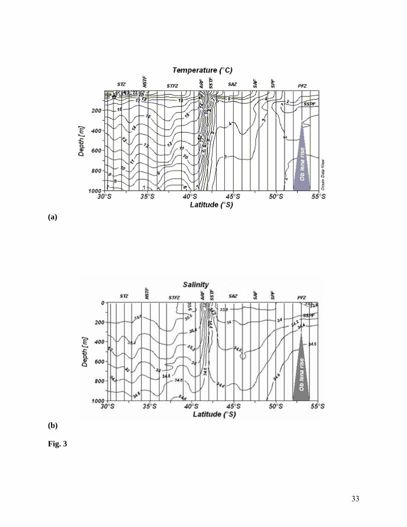
34.16) were noticed. The vertical section of temperature and salinity (Figs. 3a and b) showed that

the expression of this front extended down to 900 m. SAZ is a region where temperature

stratification was more intense compared to the salinity stratification. Compared to other regions,

salinity minimum zone was noticed in the SAZ and it was associated with AAIW. This zone is

the limit of the warm and saltier waters, typical of the subtropical regions with a thermostad (Fig.

3a) between 200 and 400 m. The temperature and salinity section (Fig. 3a and b) in the SAF

showed a weak gradient at surface between 47° and 48°S, denoting the frontal boundary between

Sub Antarctic Surface Water (SASW) and polar surface waters. The mean position of the SPF,

according to surface and subsurface expressions, was at around 50°S, where SST (Fig. 2) was

3.8°C and SSS was 33.79. We observed the sub surface polar front between 51° and 55°S with

the 2.0°C isotherm clearly demarcating the surface and subsurface expressions of the polar front.

The sections of the temperature and salinity (Figs. 3a and b) showed the northward extension of

the low temperature (< 2.0°C) and fresher water mass at depths of 100 to 400 m, where salinity

(34.2 - 34.6) remained relatively constant.

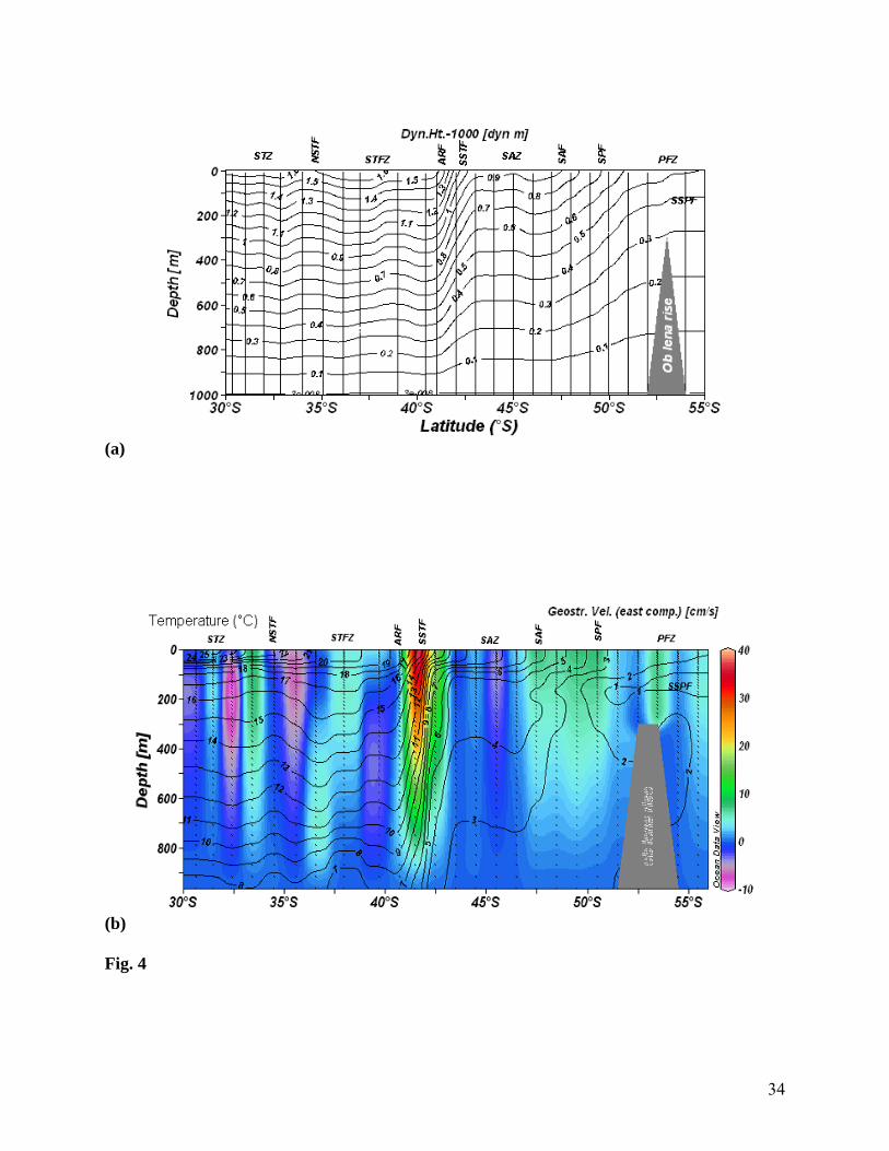
Strong, zonally prevailed westerly winds forced large, near-surface, northward Ekman

transport creating a northward pressure gradient. The ACC is approximately in geostrophic

equilibrium, with isopycnals inclined towards the surface layer of polar region. Geostrophic

currents (from thermohaline profiles) also showed strong band of eastward flowing current (40

cm s-1) between 41° and 43°S with a vertical extension of 800 m (Fig. 4b).

Surface DO values were relatively low (~225 µM) between 30 and 35°S and increased to 310

µM between 39° and 43°S (Fig. 5a). Further south, DO gradually increased to reach a maximum

of 360 µM at 54°S (Fig. 5a). Surface DO was found to be inversely correlated (r2 = 0.96) with

SST (Fig. 6a), and positively correlated (r2 = 0.324) with wind speed (Fig. 6b). Surface

10

macronutrients (Figs. 5b, c and d) were consistently low between 30° and 40°S (nitrate ~1 µM,

phosphate ~0.18 µM and silicate 6 µM). However, south of 41°S, nitrate concentrations (Fig. 5b)

rose sharply to attain a maximum of 27.5 µM at 51°S, but declined to 10 µM at 55°S. Surface

phosphate concentrations (Fig. 5c) rose south of 43°S to a maximum of 1µM, which sustained

between 49° and 53°S, but declined to 0.17µM at 55°S.

During the austral summer, the maximum intensity of solar radiation (Fig. 7a) was

calculated to be 475 to 400 watt m-2 between 30° to 55°S and the day length (Fig. 7b) increased

southwards from about 14 to 18 hr. The PAR (photosynthetically available radiation) estimated

from SeaWiFS showed a zonal pattern, with high radiation (>50 E m-2 d-1) at 30°S which

declined to < 30 E m-2 d-1 at 55°S. Calculated euphotic zone had a potential depth range of 50 -

70 m between 40° to and 50°S, and increased to 70 - 90 m equator wards. During this period, the

average surface chlorophyll a concentration (Fig. 8a) was high (1.0 mg m-3) between 41° and

43°S, but was low (0.08 mg m-3) in other areas, except at the Polar Front where it reached 0.2 mg

m-3.

The linear relation between in situ and remotely sensed chlorophyll a had a correlation (r2) of

0.43 and yielded a validation relation for remotely sensed chlorophyll a as,

Corrected remotely sensed chlorophyll = 1.83 X in situ Chl +0.03

This correction was applied to SeaWiFS chlorophyll (Fig. 8b) that showed high chlorophyll a

concentrations of >7 mg m-3 between 41° and 42°S. The linear relation between in situ and

primary productivity estimated from the Vertically Generalized Production Model (VGPM)

showed a correlation (r2) of 0.41 and yielded a validation relation for modelled primary

production as,

Corrected primary production (VGPM) =22.62 X in situ PP+98.23

Results showed a zone of high column productivity of 400 to 1000 mg C m-2 d-1 between 39° and

43°S with a maximum of 1000 mg C m-2 d-1 at 42°S (Fig. 9). Primary production rates decreased

both northwards to 20°S (to 200 mg C m-2 d-1) and southwards to 55°S (to 100 mg C m-2 d-1).

11

The microzooplankton density in the surface layer increased in the vicinity of the SPF

(139 х 103 no.m-3) and SAF (80 х 103 no.m-3), and decreased at the PFZ (2.80 х 103 no.m-3).

Frontal regions, north of the subtropical convergence (30° to 42°30’S) possessed less

microzooplankton than south. Fronts sustained relatively high microzooplankton abundance than

the zones except at SAZ where the density was79.4 х103 no.m-3. The upper 120 m also showed

more or less the same trend as that of the surface layer. Each zone and front was identified and

characterised by a unique composition of microzooplankton community (Fig.10a & b). At SPF

microzooplankton community was dominated by ciliates (53%), dinoflagellates (16%), and

nauplii (26.5%), but at SAF, the composition changed, and the contribution of ciliates fell to

19%, and that of dinoflagellates and nauplii increased to 36.5 and 25%, respectively. North of

SSTF, the contribution of ciliates (>50%) to the microzooplankton community was higher than

south of SSTF, except at SAZ (84%). The maximum contribution of ciliates (84%) to the

microzooplankton community was coinciding with that of SAZ.

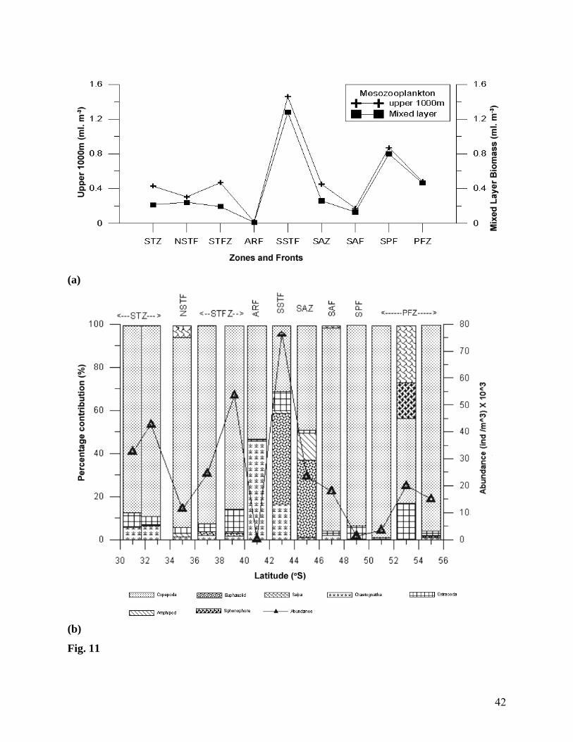
Between 30° and 55°S, high zooplankton biomass in the mixed layer was recorded at

PFZ (50° - 55°S). Among the fronts, mesozooplankton biomass was high in the mixed layer of

SSTF, between 41°15’ and 42°30’S. However, compared to all other zones and frontal regions,

mesozooplankton biomass (Figs. 11a, and b, Table 2) was extremely low (0.010 ml m-3) in the

mixed layer and in the upper 1000 m (0.018 ml m-3) of the ARF (Fig. 11a). The major

components of mesozooplankton community (Fig. 11b) in ARF were copepods (53.57%),

chaetognaths (42.86%), and ostracods (3.57%). An interesting feature observed was that in the

upper 1000 m, the mesozooplankton standing stock remained consistent between different zones

(STZ, STFZ, SAZ and PFZ), despite the variations in hydrographic conditions and

mesozooplankton composition across the fronts (Table 2). The region between SSTF (41°15’-

42°30’S) and SAZ (43°- 47°S) were characterised by high incidence of Euphausiids (68 and

49%, respectively), while in the other regions copepods formed the bulk of the community

(>90%).

4. Discussion

In the STZ, surface waters are warm (Fig. 2 and 3a), high saline (Fig. 3b) and nutrient-

poor (Fig. 5b, c and d). The subduction of these nutrient-poor surface waters as a result of the

12

anticlockwise subtropical gyral circulation, results in highly oligotrophic conditions (Karstensen

& Quadfasel 2002). The low chlorophyll a (<0.1 mg m-3) (Fig. 8) and low primary production

(< 250 mg C m-2) recorded in this region are clear indications of the oligotrophic nature of the

water (Figs. 8 & 9). This is maintained almost throughout the year except during July -

September (Fig. 8b). The seasonal variations in the solar irradiance (Figs. 7a and b) of 200 - 450

w m-2 and the day length of 9 to 15 hr indicate that the low primary production was not due to

light limitation. The most likely causes for the low primary production in the region may be the

combined effect of the low nutrient concentrations in the euphotic zone, the thermocline depth

exceeding the compensation depth and high stability due to stratification. Surprisingly, we

observed high mesozooplankton standing stock (0.440 ml m-3) in the upper 1000 m (Figs. 11a

and b) in this region despite the prevailing oligotrophy and low primary production. Incidentally,

the biomass value showed close similarity with those of STZ (0.41), STFZ (0.470 ml m-3), SAZ

(0.445 ml m-3) and PFZ (0.50 ml m-3). Microbial food web is known to support high

mesozooplankton production in the low-nutrient low chlorophyll systems (Azam 1983& 1991,

Hall et al. 1999), thereby replacing the primary producers (phytoplankton) as the source of

nutrition. The occurrence of a relatively high microzooplankton community (Figs. 10a and b),

dominated by ciliates (2203 x 103 no.m-3, 65%), indicates the possibility of strong microbial food

web operating in this region. We observed maximum density of ciliates, (2819 x 103 no. m-3) in

STZ, which was in contrast with the minimum density of ciliates (108 x 103 m-3) in the PFZ.

Bradford-Grieve et al. (1997) have reported that significant proportions of the phytoplankton

stock were of picoplankton size range, and ciliates were the dominant grazers of both the pico -

and nanoplankton. Low phytoplankton density with high abundance of picoplankton has been

reported from the subtropical north Pacific (Odate 1994). The flow cytometry data (Detmer &

Bathmann 1997) have also shown that autotrophic pico- and nanoplankton may contribute up to

90% of total chlorophyll a present in other oligotrophic regions. Under high nitrate condition,

large size classes of phytoplankton usually flourish, whereas in nitrate-depleted waters,

picoplankton predominates (Taguchi et al. 1992, Calbet et al. 2001) and this population can

support substantial amount of secondary (zooplankton) production through the microbial food

web. Thus the low availability of the large sized phytoplankton initiated the need for alternating

food sources for the mesozooplankton. The trophic role of microzooplankton, in supporting the

high mesozooplankton is evident from the high abundance of ciliates. The relatively high

13

biomass of microzooplankton indicates a very strong coupling between the mesozooplankton and

the microbial food web. Satapoomin et al. (2004) also reported the role of microzooplankton in

structuring the mesozooplankton community in oligotrophic waters.

We observed the NSTF (Belkin & Gordon 1996) between 34° and 35°S in the southern

Indian Ocean where it formed the boundary for warm, saline subtropical water and was well

expressed in subsurface features (Figs. 2, 3a and b). Primary productivity and zooplankton

biomass and abundance decreased sharply across the front (Figs. 8a, 11a, and b). Compared to

other frontal features, the biological production associated with this front was very low. The

higher abundance of microzooplankton (Figs. 10a and b) in the NSTF (3046 x 103 no.m-2) clearly

indicates the extreme oligotrophic nature of this front.

The STFZ (Lutjeharms et al. 1993) region is bounded by the NSTF to the north and the

ARF to the south. In this region biological production was low, as in the subtropical region

despite receiving ample solar irradiance and day length of sufficient duration. But, seasonal

chlorophyll a concentrations show that it is a low productivity region throughout the year.

However, the relatively high abundance of the microzooplankton (Figs. 10a and b) (2819 x 103

no.m-2) might be sufficient enough to sustain a fairly high mesozooplankton biomass, and it was

similar to the biomass values observed in the other zones. Earlier studies have indicated that the

low productivity regions were dominated by microbial food web and the major carbon flow was

through the microbial food web to the microzooplankton with a very high proportion of the

primary production being consumed by the microzooplankton (Azam 1983 &1991, Hall et al.

1999).

ARF (Lutjeharms & Valentine 1984, Belkin & Gordon 1996) is readily distinguishable

by its expression in SST that ranged from 20.7 to 17.2°C (mean 18.4°C) and in the subsurface

(upper 100-150 m) thermohaline fields. The Agulhas Retroflection Current has a core width of

~70 km and it transports an estimated 44 ±5 Sv in the upper 1000 m (Boebel et al. 2003).

Between 38° and 40°S it develops a quasi-stationary meandering pattern (wavelength 500 km).

The upwelled waters along of the southwest African coast are being advected in to the present

study area, and this could be identified by their relatively high content of nitrate (0.28 µM) (Fig.

5b), chlorophyll a (0.13 mg m-3) (Fig. 8a) and primary productivity (493 mg C m-2d-1) (Fig. 9).

14

Both chlorophyll a concentrations and primary production within the Agulhas current system

exhibited seasonal patterns (Fig. 8b). SeaWIFS data showed high chlorophyll a concentrations

(0.5 mg m-3) during the austral summer (December) (Fig. 8b). But, instead of a proportionate

increase, we observed a drastic decrease (Figs. 11a and b) in the mesozooplankton biomass in

this front. On the other hand, microzooplankton was abundant (12.8 x 103 no.m-3 ) in the surface

layer (Fig. 10a). The integrated abundance of microzooplankton in the upper 120 m (Fig. 10b)

was 2434 x 103 no.m-2 and the community was dominated by ciliates (62%). However,

elucidating the food web ecology in such complex situations is very difficult. The mixing of the

oligotrophic subtropical water with nutrient-rich Atlantic and Subantarctic waters substantially

modifies the system. In such a dynamic system, the current velocities (Boebel et al. 1998) are so

high (≈200 cm.s-1 ), that they might deter the stabilization of mesozooplankton population and/or

the time may not be sufficient for the population to respond to the nutrient enrichment.

Our observation of the mean position of the SSTF front was consistent with that of

Lutjeharms & Valentine (1984). SSTF is the boundary between the warm saline (Figs. 3a and b)

subtropical waters and the cool fresh waters of the SO. In the convergence, both chlorophyll a

and column primary production were high (0.47 mg m-3 and 950 mg C m-2d-1, respectively) and

so also the mesozooplankton standing stock (1.46 ml m-3). The isopycnal mixing between the

subtropical and subantarctic waters introduces nutrient-rich subthermocline waters into the

surface layers, thereby augmenting the primary (Fig. 9) and secondary production (Figs. 11a and

b). This also enhanced both the surface (14.4 x 103) and column (Figs. 10a and b) (4459 x 103)

microzooplankton biomass. Previous studies have recorded that frontal systems are characterized

by increased biological productivity and biomass at all trophic levels of the pelagic eco-system

(Lutjeharms et al. 1985, Pakhomov et al. 1994, Pakhomov & McQuaid 1996). The

microzooplankton community changes from being totally dominated by ciliates in the

subtropical waters to more diverse forms (ciliates 36%, dinoflagellates 38% and nauplii 25%).

This change in microzooplankton population could also be due to a change toward larger

phytoplankton favouring populations of larger heterotrophic dinoflagellates rather than ciliates.

Hansen (1991) reported the ability of heterotrophic dinoflagellates to graze a wider range of

prey, from small cyanobacteria to larger diatoms, their diverse feeding mechanisms enable them

to survive in a variety of environments. During the winter, productivity is probably light-limited,

15

and the ciliates dominate in the microzooplankton community, and the energy flow is

predominantly via the microbial loop. During the spring and summer, since light is not a limiting

factor, large phytoplankton blooms occur (Fig. 8b), which can be sustained by the nutrients

supplied by the vertical mixing of water. However, high microzooplankton populations are also

maintained at the same time implying that the microbial loop is also active during this period.

The SAZ has an almost uniform SST of 8.3°C (Figs. 2 and 3a) and SSS of 33.8 (Fig. 3b)

throughout. There is a clear thermostad (Fig. 3a) at 200 to 400 m depth, which forms in the

winter as a result of vertical overturn. This is a HNLC zone. To the north, productivity in the

subtropical waters is nutrient-limited, whereas to the south, the Polar zone is light-limited.

Within this region solar irradiance is estimated to be 150 wm-2 (day length ~9 hr) during the

winter and rises to 450 w.m-2 (day length ~15hr) during summer. Although the macronutrient

supplies in the wind mixed layer were sufficient enough to support high productivity, the surface

chlorophyll a (Fig. 8a) concentration (0.18 mg m-3) and column primary productivity (374 mg C

m-2 d-1) remained very low (Fig. 9). Two main hypotheses have been proposed to explain why

primary production remains suppressed. One hypothesis is that grazing pressure reduces the

phytoplankton abundance and the other one is that lack of essential micronutrients, particularly

iron limits the primary production (Martin et al. 1990a & 1990). Mesozooplankton standing

stocks in this region (Fig. 11a) were similar to those observed in both the subtropical and polar

zones (Fig. 11b), but microzooplankton population showed abundance at the surface (79.4 x 103

no.m-3) and in the upper 120 m column (5608 x 103 no.m-2 ) (Figs. 10a and b). This indicates that

the primary production in this region is supported by regenerated nutrients and is utilized in the

microbial food web. It has also been reported that nano-phytoplankton which supports the

microzooplankton community, was the dominant component in the inter frontal regions between

the SSTF and SAF during late summer (Laubscher et al. 1993).

SST declined from 9.0 to 5.1°C (Lutjeharms & Valentine 1984) across the SAF, and SSS

declined from 34.11 to 33.89 (Allanson et al. 1981). Belkin & Gordon (1996) defined the front as

the boundary between the intermediate salinity minimum and Sub Antarctic Mode Water

(SAMW) thermostad to the north. Despite the high concentrations of nutrients (Figs. 5b, c and d)

(NO3, 21.3, PO4, 0.96 and SiO4, 8.4), the biological production was low. During winter, low solar

irradiance (Figs. 7a and b) and the short day lengths were probably the major limiting factors on

16

productivity. But even during summer, standing stocks of chlorophyll and primary production

remained low (Figs. 8a and b) (0.2 mg m-2, 327 mg C m-2 d-1, respectively) so also the secondary

production (0.13 ml m-3, 0.173 ml m-3) (Figs. 11a and b). This finding is in agreement with

earlier studies conducted in the SSAF (Bernard & Froneman 2003). Microzooplankton

abundance both at the surface (80 x 103 no.m-3) and in the upper 120 m (3600 x 103 no.m-2)

(Figs. 10a and b) was sufficient to support moderate mesozooplankton standing stocks. The

composition of the microzooplankton community (Fig. 10b) changed (ciliates 19%;

dinoflagellates 36.5%, and nauplii 25%). This change in microzooplankton population could

also be due to a change toward larger phytoplankton favouring populations of larger

heterotrophic dinoflagellates rather than ciliates.The reduction in ciliate population was probably

related to the development of large diatom blooms, as the diatoms are too large in size for the

ciliates to feed on. The other important microzooplankton group the heterotrophic dinoflagellates

prefer prey of their own size and the linear size ratio between predators and their optimal prey is

1 : 1 and hence the prey predator size ratio is crucial for the structuring of pelagic food web

(Hansen et al. 1994). It has been observed that changes in the environmental conditions influence

the abundance and composition of the microzooplankton community (Atkinson, 1996, Hall et

al.1999). A major factor contributing to low biomass of mesozooplankton (Figs. 11a and b) may

be the changing environment, i.e. the formation of AAIW and lateral mixing with SAMW,

resulting in a sharp drop of 3.0°C in SST. The assemblage of organisms that inhabited the polar

region was entirely different from that in the subtropical seas. Even though food resources in the

front were potentially high, the sharp shifts in environmental conditions probably inhibited the

build up of the standing stocks of zooplankton.

The SPF is a region where SST changes from 6.0° to 2.0°C (mean 3.4°C) and SSS

from 33.8 to 33.9. We observed maximum SST gradient (Figs. 2 and 3a) centered at 3.8°C and

SSS at 33.79 (Fig. 3b) are in agreement with those reported by Allanson et al. (1981). One effect

of the ACC (Fig. 4a) is that it caused the isopycnals to outcrop at the surface, and hence mixing

of the high concentration of nutrients occurred from deep water to the surface layers (Sloyan &

Rintoul 2001, Pollard et al. 2002). We observed sharp increases in the nutrient concentrations

(Figs. 5b, c and d) (NO3- 26.7, PO4

- 0.8 and SiO4- 39.4) associated with the frontal region.

Seasonal fluctuations in solar irradiance and day length (Figs. 7a and b) showed that there was

absence of light during the winter, but during summer, despite the sun’s low angle of incidence

17

sufficient light was available for photosynthesis. However, no concomitant general increase in

the chlorophyll a (Fig. 8a) and water column production (Fig. 9) were observed. It is now

recognized that phytoplankton blooms associated with the seasonal ice retreat contribute

substantially to the biochemical cycling (Smith & Nelson, 1986). However, we observed low

chlorophyll a (<0.2 mgm-3) and primary production (<200 mg C m-2 d-1) (Table.1). Bernard &

Froneman (2003) have shown that no enhancement of chlorophyll a biomass was recorded in

the vicinity of PF. Froneman et al. (2000) and Pakhomov & Froneman (2004) found that

zooplankton grazing accounted for up to 89% of daily primary production in the Polar region.

Thus, in contrast to the HNLC regions, it appears that high grazing pressure by abundant

mesozooplankton standing stock (Figs. 11a and b), and increase of copepod nauplii in the

microzooplankton community (Figs. 10a and b) might have limited the build up of chlorophyll a

concentrations (phytoplankton bloom). The chlorophyll a and primary production presented here

are substantially lower than those observed in the PF by Allanson et al. (1981) and Lutjeharms et

al. (1985). De Baar et al. (1995) correlated high iron concentrations with enhanced primary

productivity at PF in the Atlantic sector. They have reported that the high primary productivity

was supported by the advection of iron-rich water masses within the frontal jet. Ciliates occurred

at maximum densities at the surface at 49°S (Fig. 10a), where the surface chlorophyll was 0.18

mg m-3. The contribution of heterotrophic dinoflagellates appears to be higher in the subsurface

layers (Fig. 10b), within the pycnocline as well as at the base of the photic zone. These depth

profiles may result from the predator/prey interactions, characteristic for microzooplankton

consumers, such as ciliates, which generally feed on particles < 20 µm. During the spring and

summer, diatoms can exploit the eutrophic conditions and develop blooms. We observed the

highest microzooplankton (Fig. 10a) abundance both at the surface (140 x 103 no.m-3) and within

the upper 120 m (Fig. 10b) (8057 x 103 no.m-2). Here the major constituents of the

microzooplankton community were ciliates (53%), nauplii (26.5%) and dinoflagellates (16%). In

late summer, both chlorophyll a (0.125mgm-3) and primary production (187 mg C m-2 d-1) levels

declined. Even then the microzooplankton community (8057 x 103) flourished and sustained high

mesozooplankton (Figs. 11a and b) standing stock (0.87 ml m-3). Low chlorophyll a and low

primary production rates with high micro- and mesozooplankton biomass establish that both

traditional and microbial loop were active in this front.

18

In the PFZ, weak subsurface salinity and temperature minimum (Fig. 2) were observed

that was concordant with the observation of Allanson et al. (1981). During the spring-summer,

ice melt and Antarctic divergent water advected from the Antarctic region stabilized the upper

water column, especially where the isopycnals outcrop because of the ACC (Fig. 4a). This

increased in water column stability with high nutrient and trace metal concentrations play a

major role in triggering phytoplankton blooms in the vicinity of the polar front (Dubischar &

Bathmann 1997, Perissinotto & Pakhomov 1998). Antarctic polar frontal zones are characterized

by patches and bands of high chlorophyll a (Laubscher et al. 1993, Dafner &Mordasova, 1994,

Bathmann et al. 1997). The growth rates and maximum standing stocks of the large diatom

appear to have been regulated by the availability of dissolved silica. Tremblay et al. (2002)

reported that along the Polar Front, elevated concentration of chlorophyll a and primary

production and abundance of microzooplankton (>20-200 µm) coincided with high dominance of

large or long chained diatoms. Strong nutrient deficits (Figs. 5b, c and d) were clearly seen in

this region. The decrease in the nutrient concentrations (NO3 - 10 µM) in this region (Figs. 5b, c

and d) was generally linked with high diatom blooms; but chlorophyll a concentrations (Fig. 8a)

and primary production (Fig. 9) did not correlate with these blooms. The high grazing pressure

of copepods and salps (Figs. 11b), which were very abundant at the time of our observations,

probably reduced the phytoplankton standing crop and productivity. The stable stratification

resulting from the advection of fresher, and ice melt water from the ice edge probably prevented

vertical mixing of deepwater and replenishment of nutrients. These studies highlight the

importance of the PF as a biogeographic boundary for zooplankton distribution, demarcating

Subantarctic and Antarctic realms of the SO. The sharp decrease in the microzooplankton

abundance in this zone may also be the result of strong grazing pressure by large copepods and

carnivorous zooplankton. Copepods were the dominant metazooplankton in the PFZ (Franz &

Gonzalaz 1997). The mesozooplankton community was dominated almost entirely by copepods,

which is in agreement with a number of previous studies (Pakhomov &Froneman 1999, Bernard

& Froneman 2003 & 2005). Within the microzooplankton community, ciliates (25%) were

replaced by copepod nauplii (50%), and this probably contributed to the strong grazing

pressures. Lugomela et al. (2001) reported that copepod nauplii are an important link between

the classical and microbial foodwebs because of their small size and have the ability to feed on

pico-sized particles,which are generally unavailable to the later copepodites and adults.The

19

strong grazing impact of copepods in the PFZ during autumn has been reported (Perissinotto

1992, Bernard & Froneman 2003) and the slightly reduced impact during summer may be

attributed to the inability of copepods to consume larger phytoplankton, which dominate total

chlorophyll a (Fortier et al.1994). The mesozooplankton biomass was 0.5 ml m-3 which was

almost equal to that observed in the other zones. Although most of the cyclopoids did not

significantly ingest small autotrophic and heterotrophic flagellates (2-8 µM), large copepods

were actively feeding on >10 µm particles including autotrophic/ heterotrophic dinoflagellates

and ciliates with a clearance rate of 0.03 to 0.38 ml animal-1 h-1 (Nakumura& Turner (1997)).

Odate (1994) suggested that top-down control of zooplankton might alter the abundance and size

composition of phytoplankton in summer, i.e. net zooplankton grazing may suppress the net

phyto- and microzooplankton abundance (Multivorous food web).

Belkin & Gordon (1996) identified the northern boundary of the subsurface minimum

layer, bounded by the 2.0°C isotherm, within the depth range of 100 to 300 m. We observed the

subsurface polar front between 51° and 55°S; the 2.0°C isotherm clearly demarcated the polar

waters at both the surface and subsurface layers. Our mean path turns southward at the Ob’-Lena

Rise (46°E). Seamounts and islands are regions of locally enhanced production through the

‘island mass effect’ (Genin & Boelhert 1985, Coutis & Middleton 1999), and in HNLC regions

by being a source of dissolved iron. The high mesozooplankton abundance (12.8 ml m-3) (Figs.

11a and b, Table 2) found observed in this region may be due to the island mass effect. The

major contributors of this high biomass were copepod, salps and medusae.

5. Conclusions

This study revealed that during the austral summer, mesozooplankton-standing stock

remained more or less similar in all zones (STZ, STFZ, SAZ and PFZ) of Indian Ocean sector of

Southern Ocean crossing 45°E meridian, though chlorophyll a and primary production varied in

each zone. The similarity in the mesozooplankton standing stock can be attributed to the

functioning of alternate food webs like microbial loop and multivorous food web. A chart of

solar irradiance and day length showed that light was not a limiting factor for biological

productivity in the subtropical region, whereas it was a constraint in the Subantarctic and Polar

regions. While nutrient was the major limiting factor for primary production in the photic zone of

20

Subtropical region, solar irradiance was the cause in the Subantarctic and Polar Frontal zones.

Oligotrophic behavior of Subtropical region was due to the combined effect of low nutrient

concentration in the surface layers, deep thermocline region that exceeded compensation depth

and strong stratifications. Although such a condition existed in this region, microbial food web

played a vital role in maintaining the zooplankton standing stock through high ciliate abundance.

Thus, the basic metabolic needs of the mesozooplankton were met by grazing microzooplankton.

The dominance of the microzooplankton in the subtropical region is supported by the findings of

-Grieve et al. (1997). In the Agulhas region, availability of sufficient amount of nutrients and

primary production made the system eutrophic, but the secondary standing stock was found to be

quite low. This may be due to the prevalence of strong currents and dynamic environment,

deterring the establishment of mesozooplankton communities. Due to the strong circumpolar

current and weak stratification maintained by tilting of isopycnals towards surface in the

southern part of ACC, permanent thermocline reached the surface of SSTF and supplied very

high amount of nutrients and CO2 which could be utilized for biological production. High rates

of primary and secondary production suggest the prevalence of active traditional food web and

high abundance of microzooplankton community indicates the functioning of active microbial

foodweb also in this front. Subantarctic zone exhibited HNLC phenomenon, but

mesozooplankton abundance in this zone was more or less similar to other zones. This was due

to the abundance of microzooplankton which provided the nutritional resources for the

mesozooplankton. Polar frontal zone becomes productive during austral summer by a combined

effect of advection of ice melt and Antarctic divergent water together with trace metal

concentration and stabilized upper water column. However, high grazing pressure exerted by

copepods and tunicates decreases the phytoplankton standing stock in the PF, and the prevalence

of a multivorous food web maintained a secondary standing stock similar to that of other zones.

This was well supported by replacement of ciliates by copepod nauplii in the microzooplankton

community. From the study it is understood that the similarity in the mesozooplankton standing

stock in all the major zones are supported by microzooplankton community. In the zones, the

major share of the primaryproduction could be channelled through the microzooplankton in

sustaining the mesozooplankton biomass.This illustartes the importance of the microbial food

web as a link for the transfer of carbon fixed by small autotrophs to

mesozooplankton.Nonetheless, only long-term observations can clearly show whether

21

seasonality has any impact on the mesozooplankton standing stock. Further studies in this

direction would give a better understanding of the intricate relationship underlying the secondary

productivity of the Southern Ocean.

Acknowledgements

We thank the Director, National Institute of Oceanography, Goa and the Director, Centre for

Marine Living Resources and Ecology, Kochi and the National centre For Antarctic and Ocean

Research, Goa for providing facilities for the study. We are grateful to Dr. K. Banse, School of

Oceanography, University of Washington, Seattle, USA and Dr. M.V. Angel, Southampton

Oceanographic Centre, UK for critically reading the manuscript. We also thank all the

participants of cruise SK 200 of ORV Sagar Kanya for the help rendered in sampling. The

anonymous reviewers are greatly acknowledged for their valuable suggestions,

which improved the quality and clarity of the manuscript. This investigation was

carried out under the pilot expedition to Southern Ocean funded by Ministry of Earth Sciences,

Govt. of India, New Delhi.

References

Abrams R W (1985a) Energy and food requirements of pelagic aerial seabirds in different regions of the African sector of the Southern Ocean. In:Siegfried WR, Condy PR, Laws RM (eds) Antarctic nutrient cycles and foodwebs. Springer,Berlin Heidelberg New York: 466-472

Allanson BR, Hart RC, Lutjeharms JRE (1981) Observations on the nutrients, chlorophyll and primary production of the Southern Ocean south of Africa. South Afr J Ant. Sci 10/11:3-14

Atkinson A (1996) Sub Antarctic copepods in an oceanic low chlorophyll environment: Ciliate predation, low food selectivity and impact on prey populations. Mar Ecol Prog Ser 130:85-96

Azam F, Fenchel T, Field JG, Gray JS, Meyer-Reil LA, Thingstad F (1983) The ecological role

of water-column microbes in the sea. Mar Ecol Prog Ser 10:257-263

Azam F, Smith DC, Holli baugh JT (1991) The role of the microbial loop in Antarctic pelagic

22

ecosystems. Polar Res 10:239-243

Bathmann UV, Scharek R, Klaas C, Dubischar CD, Smetacek V (1997) Spring development of phytoplankton biomass and composition in major water masses of the Atlantic sector of the Southern Ocean. Deep- Sea Res II 44: 51-67

Behrenfield MJ, Falkowski PG (1997a) A consumer’s guide to phytoplankton primary productivity models. Limnol Oceanogr 42:1479-1491

Behrenfield M J, Falkowski P G (1997b) Photosynthetic rates derived from satellite – based chlorophyll concentration. Limnol Oceanogr 42: 1-20

Belkin IM, Gordon A L (1996) Southern Ocean fronts from the Greenwich Meridian to Tasmania. J Geophys Res 101: 3675-3696

Bernard KS, Froneman PW (2003) Mesozooplankton community structure and grazing impact in

the Polar Frontal Zone of the south Indian Ocean during austral autumn 2002. Polar Biol 26:268-275

Bernard KS, Froneman PW (2005) Trophodynamics of selected mesozooplankton in the west-

Indian sector of the Polar Frontal Zone, Southern Ocean. Polar Biol 28:594-606

Boebel O, Rossby T, Lutjeharms J, Zenk W, Barron C (2003) Path and variability of the

Agulhas Return Current. Deep-Sea Res II 50:35-56

Boebel O, Rae CD , Garzoli S , Lutjeharms J, Richardson P, Rossby T, Schmid C, Zenk W, (1998) Float experiment studies interocean exchanges at the tip of Africa. EOS, 79: 7-8

Boyd P W, Watson A J, Law C S, Abraham ER, Trull T, Murdoch R, Bakker DCE, Bowie AR , Buesseler KO, Chang H, Charett M, Croot P, Downing K, Frew R, Gall M, Hadfield M, Hall J, Harvey M, Jameson G, LaRoche J, Liddicoat M, Ling R, Maldonado MT, McKay RM, Nodder S, Pickmore S, Pridmore R, Rintoul S, Safi K, Sutton P, Strzepek R, Tanneberger K, Turner S, Waite A, Zeldis J (2000) A mesoscale phytoplankton bloom in the polar Southern Ocean stimulated by iron fertilization. Nature 407:695-730

Bradford-Grieve JM, Chang FH , Gall M, Pickmere S, Richards F (1997) Size fractionated phytoplankton standing stocks and primary production during Austral winter and spring 1993 in the subtropical convergence near New Zealand. New Zealand J Mar Freshwater Res 31: 201-224

Calbet A, Landry M R, and Nunnery S (2001) Bacteria flagellate interactions in the microbial

food web of the oligotrophic subtropical North Pacific. Aquatic Microb Ecol 23: 283-292

Carpenter J H (1965) The Chesapeake Bay Institute technique for the Winkler

23

dissolved oxygen method. Limnol Oceanogr 10: 141-143.

Coutis PF, Middleton J H (1999) Flow topography interaction in the vicinity of an isolated deep ocean island. Deep- Sea Res II 46:1633-1652

Dafner EV, Mordasov NV (1994) Influence of biotic factors on the hydro chemical structure of surface water in the polar frontal zone of the Atlantic Antarctic. Mar Chem 45: 137-148

De Baar H J W, de Jong J T M, Baker D C E (1995) Importance of iron for plankton blooms

and carbon dioxide draw down in the Southern Ocean. Nature 373: 412 – 415

Deacon GER (1933) A general account of the hydrology of the South Atlantic Ocean. Discovery Report 7: 171-238

Deacon GER (1937) The hydrology of the Southern Ocean. Discovery Report 15: 122 -123

Deacon GER (1982) Physical and biological zonation in the Southern Ocean. Deep- Sea Res II 29:1-16

Deacon G ER (1983) Kerguelen, Antarcic and Subantarctic. Deep- Sea Res I 30: 1-15

Detmer A, Bathmann U (1997) Distribution patterns of autotrophic pico- and nanoplankton and their relative contribution to algal biomass during spring in the Atlantic sector of the Southern Ocean. Deep-Sea Res II 44: 299-320

Dubischar CD, Bathmann UV (1997) Grazing impact of copepods and salps on phytoplankton in the Atlantic sector of the Southern Ocean. Deep- Sea Res II 44: 415-433

El-Sayed S (1984) Productivity of the Antarctic waters – A reappraisal. In: Holm-Hansen O,

Bolis L, Gilles R (eds) Marine Phytoplankton and productivity. Springer, Berlin

Heidelberg, New York: p19-34

Fielding S, Ward P, Pollard R T , Seeyave S, Read J F, Hughes J A, Smith T, Castellani C (2007) Community structure and grazing impact of mesozooplankton during late spring/early summer 2004/2005 in the vicinity of the Crozet Islands (Southern Ocean). Deep-Sea Res II 54: 2106–2125

Fortier L, Le Fevre J, Legendre L (1994) Export of biogenic carbon to fish and to the deep

ocean: the role of large planktonic microphages. J Plankton Res 16:809–839

Franz HG, Gonzalez SR (1997) Latitudinal metazoan plankton zones in the Antarctic Circumpolar current along 6°W during austral spring 1992. Deep- Sea Res II 44: 395-414

24

Fronemann PW, Pakhomov EA, Perissinotto R, McQuaid CD (2000) Zooplankton structure and grazing in the Atlantic sector of the Southern Ocean in late austral summer 1993. Part 2. Biochemical zonation. Deep- Sea Res I 47:1687-1702

Froneman PW, Ansorge IJ , Richoux N, Blake J, Daly R, Sterley J, Mostert B, Heyns

E,Sheppard J,Kuyper B, Hart N, George C, Howard J, Mustafa E, Pey F, Lutjeharms JRE (2007) Physical and biological processes at the subtropical convergence in the south-west Indian ocean. South Afr J Sci 103:193-195

Genin A, Boehlert GW (1985) Dynamics of temperature and chlorophyll structures above a seamount: an oceanic experiment. J Mar Res 43: 907-924

Gordon AL (1985) Indian–Atlantic transfer of thermocline water at the Agulhas retroflection. Science 227: 1030–1033

Grachev DG (1991) Frontal zone influences on the distribution of different zooplankton groups in the central part of the Indian sector of the Southern Ocean, Samolova, M.S. and S.O.Shumkova (Ed.) Ecology of Commercial Marine Hydrobionts. TINRO Press, Vladivostok: p19-21

Grasshoff K (1983) Methods of seawater analysis. Edited by K. Grasshoff. M. Ehrhardt

and K.Kremling. (2nd Edn.), Verlag Chemie, Weinheim: p419

Hansen P J (1991) Quantitative importance and trophic role of HDS in a coastal pelagic food

web. Mar Ecol Progr Ser 73: 253–273

Hansen B, Bjornsen PK , Hansen PJ (1994) The size ratio between planktonic predators

and their prey. Limnol Oceanogr 39(2):395-403

Hall JA, James MR, Bradford-Grieve JM, (1999) Structure and dynamics of the pelagic

microbial food web of the Subtropical Convergence region east of New Zealand. Aquat Microb Ecol 20:95-105

Holliday NP, Read JF (1998) Surface oceanic fronts between Africa and Antarctica. Deep- Sea Res I 45: 217-238

Huntley ME, Lopez M DG, Karl DM (1991) Top predators in the Southern Ocean: a major leak in the biological carbon pump. Science 253:64-66.

Jaspers C, Nielsen T G, Carstensen J, Hopcroft R R, Moller E F (2009) Metazooplankton distribution across the Southern Indian Ocean with emphasis on the role of Larvaceans. J Plankton Res 31(5):525-540

25

Jones EP, Nelson DM, Treguer P (1990) Chemical Oceanography. In: Polar Oceanography Part B Chemistry, Biology and Geology, W.O.Smith, Jr. (Ed.) Academic Press, San Diego: p407-476

Karstensen J, Quadfasel D (2002) Water subducted into the Indian Ocean subtropical gyre.

Deep Sea Res 49: 1441–1457

Kostianoy AG, Ginzburg AI, Lebedav S A, Frankignoulle M , Delille B (2003) Fronts and

Mesoscale Variability in the Southern Indian Ocean as Inferred from the TOPEX/POSEIDON and ERS-2 Altimetry Data. Oceanol 43: 632–642

Kostianoy AG, Ginzburg AI, Frankignoulle M, Delille B (2004) Fronts in the Southern Indian

Ocean as inferred from satellite sea surface temperature data. J Mar Sys 45: 55-73

Laubscher RK, Perissinotto R, McQuaid CD (1993) Phytoplankton production and biomass at frontal zones in the Atlantic sector of the Southern Ocean. Polar Biol 13: 471-481

Lugomela C, Wallberg P, Nielsen TG (2001) Plankton composition and cycling of carbon during

the rainy season in a tropical coastal ecosystem, Zanzibar, Tanzania. J Plank Res 23 (1): 1121-1136

Lutjeharms JRE (1981) Spatial scales and intensities of circulation in the ocean areas adjacent to South Africa. Deep- Sea Res II 28:1289-1302

Lutjeharms JRE, Valentine HR (1984) Southern Ocean thermal fronts south of Africa. Deep- Sea Res Part A 31: 1461-1475

Lutjeharms JRE, Walters NM, Allanson BR (1985) Oceanic frontal systems and biological enhancement. In: W.R. Siegfried, (Ed.), Antarctic Nutrient Cycles and Food webs. Springer, Berlin: p 11-21

Lutjeharms JRE, Valentine HR, van Ballegooyen, RC, (1993) The Subtropical Convergence in the South Atlantic Ocean. South Afr J Sci 89:552-559

Martin JH, Fitzwater SE, Gordon RM, (1990) Iron deficiency limits plankton growth in Antarctic waters. Global Biogeochem Cycles 4:5-12

Martin JH, Gordon RM, Fitzwater SE (1990a) Iron in Antarctic waters. Nature 345: 156-158

Morel A, Berthon J (1989) Surface pigments, algal biomass profiles, and potential production of the euphotic layer: Relationships reinvestigated in view of remote-sensing applications. Limnol Oceanogr 34: 1545 - 1562

26

Nakumura Y, Turner J T (1997) Predation and respiration by the small cyclopoid copepod Oithona similis; How important is feeding on ciliates and Heterotrophic flagellates? J Plankt Res 19: 1275-1288

Nelson DM, Smith Jr, WO (1991) Sverdrup re-visited: critical depths, maximum chlorophyll levels, and the control of Southern Ocean productivity by the irradiance-mixing regime. Limnol Oceanogr 36: 1650-1661

Nielsen TG, Bjornsen P K, Boonruang P, Fryd M, Hansen P J, JanekarnV, Limtrakulvong V,

Munks P, Hansen O S, Satapoomin S, Sawangarreruks S, Thomsen H A, Ostergaard J B (2004) Hydrography, bacteria and protist communities across the continental shelf and shelf slope of the Andaman Sea (NE Indian ocean). Mar Ecol Prog Ser 274:69–86

Odate T (1994) Plankton abundance and size structure in the northern North Pacific Ocean, early summer. Fish Oceanogr 3: 267–278

Pakhomov EA, Perissinotto R, Mc Quaid CD (1994) Comparative structure of the macrozooplankton and micro nekton communities of the Subtropical and Antarctic Polar Fronts. Mar Ecol Prog Ser 111: 155-169

Pakhomov EA, McQuaid CD (1996) Distribution of surface zooplankton and seabirds across the Southern Ocean. Polar Biol 16: 271-286

Pakhomov E A and Froneman P W (1999) Macroplankton/ micronekton dynamics in the

vicinity of the Edward Islands(Southern Ocean). Mar Biol 134:501-515

Pakhomov EA, Perissinotto R, McQuaid CD, Froneman PW (2000) Zooplankton structure and grazing in the Atlantic sector of the Southern Ocean in late austral summer 1993 Part 2 Biochemical zonation. Deep- Sea Res I 47: 1687-1702

Pakhomov EA, Froneman PW (2004) Zooplankton dynamics in the eastern Atlantic sector of the Southern Ocean during the austral summer 1997/1998, Part2 Grazing impact. Deep- Sea Res II 51: 1663-1686

Perissinotto R (1992) Mesozooplankton size –selectivity and grazing impact on the phytoplankton community of the Prince Edward Archipelago (Southern Ocean). Mar Ecol Prog Ser 79: 243-258

Perissinotto R, Pakhomov E A (1998) The trophic role of the tunicate Salpa thompsoni in the Antarctic marine ecosystem. J Mar Syst 17: 361-374

Pollard RT, Read JF (2001) Circulation pathways and transport of the Southern Ocean in the vicinity of the Southwest Indian Ridge. J Geophys Res 106: 2881-2898

27

Pollard RT, Bathmann U, Dubischar C, Read JF, Lucas M (2002) Zooplankton distribution and behaviour in the Southern Ocean from surveys with a towed optical Plankton Counter. Deep- Sea Res II 42:641-673

Sakshaug E, Slagstad D, Holm-Hansen O (1991) Factors controlling the development of phytoplankton blooms in the Antarctic Ocean - a mathematical model. Mar Chem 35: 259–271

Satapoomin S, Nielsen T G, Hansen P J (2004) Andaman Sea copepods: spatio-temporal

variations in biomass and production, and role in the pelagic food web. Mar Ecol Prog Ser 274: 99–122

Sathyendranath S, Platt T (1988) The spectral irradiance field at the surface and in the interior of the ocean: A model for applications in oceanography and remote sensing. J Geophy Res 93: 9270-9280

Sloyan BM, Rintoul SR (2001) Circulation, renewal and modification of Antarctic mode and Intermediate water. J Phys Oceanogr 31:1005-1030

Smith WO Jr, Nelson DM, (1986) Importance of ice edge phytoplankton production in the Southern Ocean. Biol Sci 36, 251-257.

Strickland JDH, Parsons TR (1972) A practical handbook of seawater analysis. Bull Fish Res

Board Can, Ottawa 167: pp310

Taguchi SH, Saito H, Kasai T, Kono T, Kawasaki Y (1992) Hydrography and spatial variability in the size distribution of phytoplankton along the Kurilie islands in the Western sub Arctic Pacific Ocean. Fish Oceanogr 1: 227-237

Tremblay JE, Lucas MJ, Kattner G, Pollard R, Strass VH, Bathmann UV (2002) Significance of the Polar Frontal Zone for large-sized diatoms and new production during summer in the Atlantic sector of the Southern Ocean. Deep- Sea Res II 49: 3793-3811

UNESCO (1994) Protocols for the joint global ocean flux study, Manual and Guides. 29:

pp190

28

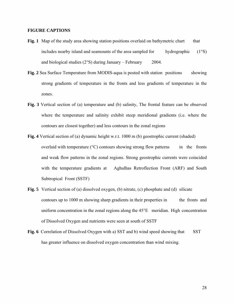
FIGURE CAPTIONS

Fig. 1 Map of the study area showing station positions overlaid on bathymetric chart that

includes nearby island and seamounts of the area sampled for hydrographic (1°S)

and biological studies (2°S) during January – February 2004.

Fig. 2 Sea Surface Temperature from MODIS-aqua is posted with station positions showing

strong gradients of temperature in the fronts and less gradients of temperature in the

zones.

Fig. 3 Vertical section of (a) temperature and (b) salinity, The frontal feature can be observed

where the temperature and salinity exhibit steep meridional gradients (i.e. where the

contours are closest together) and less contours in the zonal regions

Fig. 4 Vertical section of (a) dynamic height w.r.t. 1000 m (b) geostrophic current (shaded)

overlaid with temperature (°C) contours showing strong flow patterns in the fronts

and weak flow patterns in the zonal regions. Strong geostrophic currents were coincided

with the temperature gradients at Aghulhas Retroflection Front (ARF) and South

Subtropical Front (SSTF)

Fig. 5 Vertical section of (a) dissolved oxygen, (b) nitrate, (c) phosphate and (d) silicate

contours up to 1000 m showing sharp gradients in their properties in the fronts and

uniform concentration in the zonal regions along the 45°E meridian. High concentration

of Dissolved Oxygen and nutrients were seen at south of SSTF

Fig. 6 Correlation of Dissolved Oxygen with a) SST and b) wind speed showing that SST

has greater influence on dissolved oxygen concentration than wind mixing.

29

Fig. 7 Seasonal patterns of (a) solar irradiance and (b) Day length showing during the study

period (austral summer) light is not a constraint for the biological production in the study

area.

Fig. 8 (a) SeaWiFS Chlorophyll a (mg m-3) concentration overlaid with AVHRR SST contours

during the study period. Maximum chl a concenteration was seen in the SSTF and

minimum was at Subtropical zone. (b) Monthly distribution of SeaWiFS chlorophyll a

along 45°E from June 2003 to June 2004 showed highest chl a concenteration was during

Nov- Feb.

Fig. 9 Water column primary productivity computed from remotely sensed data by using

VGPM model also showed the high primary production rate was at SSTF.

Fig. 10 Variations in the composition of microzooplankton in the (a) surface (b) upper 120 m of

different fronts and zones .

Fig. 11 (a) Variations in the mesozooplankton biomass in fronts and zones, Uniform biomass can

be observed at different zones (b) Percentage composition of different taxa and total

abundances of mesozooplankton. Copepods were the dominant component in all of the

zones and fronts except at SSTF and SAZ

30

Table 1 Surface values of physical (Temperature (°C), Salinity) and chemical (Dissolved

oxygen & nutrients) variables measured across the fronts and zones of the 45° E

longitude during austral summer 2004. Nutrient levels and dissolved oxygen are

expressed in µM.

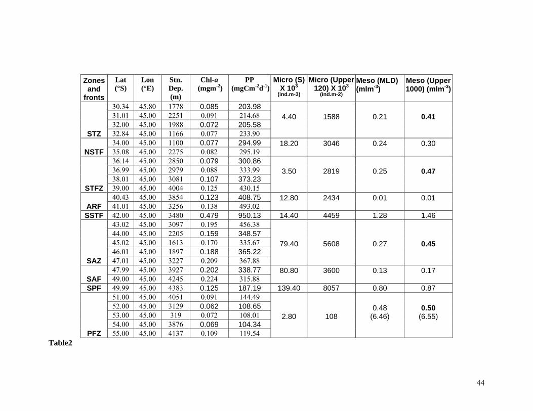
Table 2 Biological variables measured across the fronts and zones of 45° E longitude during

austral summer 2004. Variables such as chlorophyll a, Primary productivity,

microzooplankton abundance in the surface and in the upper 120 m, mesozooplankton

biomass in the mixed layer and in the upper 1000 m are shown. Biomass values

shown in bold letters are those which are more or less having same values in different

zones.

31

Figures

Fig. 1

32

Fig. 2

33

(a)

(b) Fig. 3

34

(a)

(b) Fig. 4

35

(a)

Fig. (b)

36

(c)

(d) Fig. 5

37

(a)

(b) Fig. 6

38

0

100

200

300

400

500

600

mW/m

2Lat 1

Lat 1

Lat 3

Lat 4

Lat 5

Lat 6

(a)

(b)

Fig. 7

0

24

6

8

1012

14

16

1820

Hours

Lat 1

Lat 1

Lat 3

Lat 4

Lat 5

Lat 6

39

(a)

(b) Fig. 8

40

Fig. 9

41

(a)

(b)

Fig. 10

42

(a)

(b)

Fig. 11

43

Zones and

fronts

Lat (°S)

Lon (°E)

Stn. Dep. (m)

Tpot-0 (°C)

Salinity

DO (µM)

NO3 (µM)

PO4 (µM)

SiO4 (µM)

STZ

30.34 45.80 1778 25.31 35.63 221 31.01 45.00 2251 25.14 35.66 209 2.66 0.16 6.58 32.00 45.00 1988 25.00 35.68 215 32.84 45.00 1166 23.35 35.69 223 0.66 0.16 5.17

NSTF

34.00 45.00 1100 21.92 35.69 225 35.08 45.00 2275 22.22 35.70 225 0.66 0.16 4.39

STFZ

36.14 45.00 2850 21.07 35.68 232 36.99 45.00 2979 20.05 35.64 229 0.28 0.16 7.31 38.01 45.00 3081 20.05 35.62 224 39.00 45.00 4004 20.48 35.59 219 0.43 0.16 8.04

ARF

40.43 45.00 3854 18.71 35.60 230 41.01 45.00 3256 18.42 35.62 239 0.29 0.10 5.85

SSTF 42.00 45.00 3480 13.06 34.16 286

SAZ

43.02 45.00 3097 10.23 33.70 307 14.40 0.10 9.50 44.00 45.00 2205 8.66 33.77 319 45.02 45.00 1613 8.43 33.77 307 19.73 0.64 9.50 46.01 45.00 1897 7.75 33.80 315 47.01 45.00 3227 7.24 33.79 317 19.87 0.32 7.31

SAF

47.99 45.00 3927 5.39 33.77 304 49.00 45.00 4245 5.23 33.77 335 21.31 0.96 8.04

SPF 49.99 45.00 4383 3.83 33.79 338

PFZ

51.00 45.00 4051 2.72 33.87 347 26.74 0.80 39.47 52.00 45.00 3129 2.64 33.88 340 53.00 45.00 319 2.35 33.80 350 25.88 0.96 48.97 54.00 45.00 3876 2.19 33.78 363 55.00 45.00 4137 2.24

33.80

326

10.11 0.16 24.12

Table 1

44

Zones and

fronts

Lat (°S)

Lon (°E)

Stn. Dep. (m)

Chl-a (mgm-2)

PP (mgCm-2d-1)

Micro (S) X 103

(ind.m-3)

Micro (Upper 120) X 103

(ind.m-2)

Meso (MLD) (mlm-3)

Meso (Upper 1000) (mlm-3)

STZ

30.34 45.80 1778 0.085 203.98 4.40

1588

0.21

0.41

31.01 45.00 2251 0.091 214.68 32.00 45.00 1988 0.072 205.58 32.84 45.00 1166 0.077 233.90

NSTF 34.00 45.00 1100 0.077 294.99 18.20

3046

0.24

0.30

35.08 45.00 2275 0.082 295.19

STFZ

36.14 45.00 2850 0.079 300.86 3.50

2819

0.25

0.47

36.99 45.00 2979 0.088 333.99 38.01 45.00 3081 0.107 373.23 39.00 45.00 4004 0.125 430.15

ARF 40.43 45.00 3854 0.123 408.75 12.80

2434

0.01

0.01

41.01 45.00 3256 0.138 493.02 SSTF 42.00 45.00 3480 0.479 950.13 14.40 4459 1.28 1.46

SAZ

43.02 45.00 3097 0.195 456.38

79.40

5608

0.27

0.45

44.00 45.00 2205 0.159 348.57 45.02 45.00 1613 0.170 335.67 46.01 45.00 1897 0.188 365.22 47.01 45.00 3227 0.209 367.88

SAF 47.99 45.00 3927 0.202 338.77 80.80

3600

0.13

0.17

49.00 45.00 4245 0.224 315.88 SPF 49.99 45.00 4383 0.125 187.19 139.40 8057 0.80 0.87

PFZ

51.00 45.00 4051 0.091 144.49

2.80

108

0.48 (6.46)

0.50 (6.55)

52.00 45.00 3129 0.062 108.65 53.00 45.00 319 0.072 108.01 54.00 45.00 3876 0.069 104.34 55.00 45.00 4137 0.109 119.54

Table2