1

Health Monitoring of Li-ion Battery Systems: AMedian Expectation Diagnosis Approach (MEDA)Haris M. Khalid, Member, IEEE, Qadeer Ahmed, Member, IEEE, and Jimmy C.-H. Peng, Member, IEEE

Abstract—The operations of Li-ion Battery Management System (BMS)are highly dependent on installed sensors. Malfunctions in sensors couldlead to a deterioration in battery performance. This paper proposed aneffective health monitoring scheme using a median expectation-based diag-nosis approach (MEDA). MEDA calculates the median of a possible set ofvalues, rather than taking their weighted average as in the case of a stan-dard expected mean operator. Furthermore, a smoother was developed tocapture important patterns in the estimation. The resulting filter was firstderived using a one-dimensional system example, where the iterative con-vergence of median-based proposed filter was proved. Performance evalu-ations were subsequently conducted by analyzing real-time measurementscollected from Li-ion battery cells used in Hybrid Electric Vehicles (HEV)and Plug-in HEVs (PHEV) duty cycles. Results showed the proposed filterwas more effective and less sensitive to small sample size and curves withoutliers.

Index Terms—Battery diagnosis, Battery Management System (BMS),expected value, Kalman filter, lithium-ion batteries, mean, median.

ACRONYMS AND ABBREVIATIONSBMS Battery Management System

MEDA Median expectation-based diagnosis approachHEV Hybrid Electric Vehicle

PHEV Parallel Hybrid Electric VehicleSoC State-of-chargeTMS Thermal Management SystemVMS Voltage Management SystemSMS Safety Management SystemBCU Battery Control Unit

ME-based KS Median expectation-based Kalman smootherMKF Median Kalman filterMKS Median Kalman smootherDT Detection time

MDR Missed Detection RateFDR False Detection Rate

IT Isolation timeMIR Missed Isolation RateEKF Extended Kalman filterMSE Mean Square ErrorDST Dynamic Stress rate

I. INTRODUCTION

LITHIUM-ION batteries are popular in HEV market due totheir high energy density and low maintenance cost [1–4].

However, their high capacity and large serial-parallel numbersof automotive lithium-ion batteries raised issues such as safety,reliability, cost, and uniformity. Lithium-ion batteries must op-erate in a reliable and safe operational range to prevent a de-crease in lifetime, capacity, and safety related problems [5, 6].For example, an extremely low-voltage or over-discharged bat-tery may result in the collapse of the lattice and reduction ofthe electrolyte. High temperature operation can also cause thebattery electrolyte to decompose, and produce combustible gas,

This work was developed on the data generated from the Center of Automo-tive Research Laboratory, Ohio State University, USA. The experiments weresupport by US DOE CERC under the project no. 60029877.

H. M. Khalid and J. C.-H. Peng are with the Department of Electrical En-gineering and Computer Science, Institute Center for Energy, Masdar Insti-tute of Science and Technology (MIST), Abu Dhabi, UAE. E-mail: mkhalid,jpeng@masdar.ac.ae

Q. Ahmed is with the Center for Automotive Research, The Ohio State Uni-versity (OSU), Columbus, OH, USA. E-mail: ahmed.358@osu.edu

which exothermically reacts with the oxygen generated from thedecomposition of the positive electrode. This may result in fireand thermal runaway [7–9]. On the other hand, low temperatureoperations can cause the breakdown of the cathode, and resultin short-circuit [5, 10, 11]. Meanwhile, the imprecise calcula-tion of SoC can easily trigger the overcharge or over-dischargesituation, which may result in poor HEV efficiency [12, 13].

To keep the Li-ion battery system safe from these known is-sues, BMS is required to continuously track the battery perfor-mance with the help of on-board sensors. A battery pack isgenerally composed of several modules consisting of cells con-nected in-series to provide the desired voltage and in parallelto satisfy the capacity requirements. BMS includes the follow-ing subsystems and functions: 1) a TMS to keep the batteryat optimal average temperature while minimizing temperaturedifferences among cells, 2) a VMS to reduce cell-to-cell im-balances in voltage and SoC, 3) a SMS to electrically discon-nect the battery in case of adverse conditions, and 4) a BCU.BCU controls all three subsystems, estimates battery parame-ters, and provides diagnostic and prognostic functions. This isdone using a set of current, voltage, and temperature sensorsconnected to the BCU. It can be observed that BMS operationsare highly dependent on healthy sensors. Any fault in these sen-sors, which are often neglected, can result in fatal consequences[5]. Some works were proposed for component-level analysis offaults [14–18]. However, limited attentions were given to sen-sor fault diagnosis for lithium-ion battery system at the system-level. This may lead to a false assumption that measurementscollected from sensors are always accurate within subsystems.Therefore, this paper focuses on diagnosing system-level faults.This could provide access to have traceability against the sys-tem requirements established at each component-level. It couldalso provide the dynamic aspects of component interactions, en-suring component-level compatibility with the main system.

The contribution of this paper is to enhance the reliability oflithium-ion batteries at system-level by improving the estima-tion and detection capabilities of instant nonlinear faults in theforms of spikes and outliers. This was accomplished by firstextracting the correlation information of the estimates. Sub-sequently, fault detection and isolation were performed usinga proposed fault diagnosis scheme. The proposed scheme isnamed as MEDA approach. It is based on the principles ofKalman filter, which is widely applied for monitoring and es-timating applications [19–25]. However, estimators developedfrom classic Kalman filter take the weighted average betweenthe noisy observations and the prior measurements. This min-imizes the expected value of the sample to be estimated, butdoes not guarantee a better measure of the central tendency ifthe sample size is small or contain outliers. To overcome thislimitation, a novel nonlinear filter was derived using the median

2

expected value. The proposed enhancement was incorporatedinto the estimation step and integrated with a fault diagnosisscheme to monitor lithium-ion battery system.

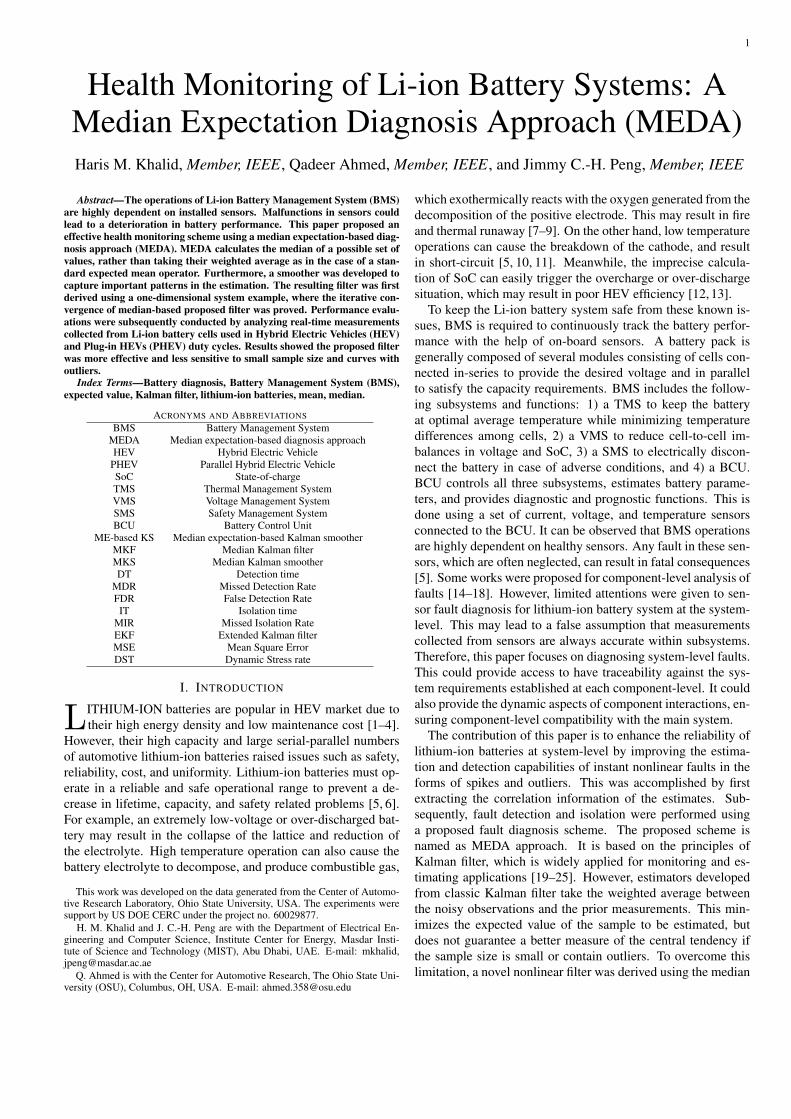
An overview of the proposed MEDA scheme is illustrated inFig. 1. Compared with its Kalman predecessors of [16] and [17]used in the same field, the proposed scheme improved the esti-mation and detection accuracy under random fault fluctuations.This was done by computing modal parameters from the inputof a variable battery system, which is the current. Subsequently,estimation of voltage and temperature outputs of the battery sys-tem was computed using a ME-based KS estimator using (25)–(28), where derivations of the equations will be shown in thefollowing sections. At this stage, random faults were injectedin both outputs. The proposed filter was applied to detect thesefaults, thereby doing a residual generation using (29)–(37). Theresidual is a measure used to quantify the existence of a fault. Tomake residual evaluation of the signal, a fault threshold selec-tion was also formulated using a coherence function (38)–(42).Once an accurate threshold was selected, faults could be iso-lated using a recognition model from (43). The isolation signalwas represented on a binary scale.

The paper is organized as follows: The problem was formu-lated in Section II. The implementation and evaluation of thescheme were discussed in Section III. Conclusions and futurework were drawn in Section IV.

II. PROBLEM FORMULATION

A. Median Expectation-Based Kalman filter with GaussianDistributions

The derivation of the median expectation-based Kalman filtermodel assumed the state x of the battery system at a time t+1evolved from its prior state at time t as:

xt+1 = Ftxt +Btut +Gtwt, t= 0,1, ...., T (1)

where x0 ∈ IRr is the initial condition of the state, and Ft ∈IRr×r is a model matrix of the state response. Note each statedepends on its covariates. The variableBt is the input transitionmatrix, ut is the input vector, Gt is the noise transition matrix,and wt ∈ IRr is the random process noise. Finally, t is the timeinstant, and T refers to the number of time instants. Let thebattery system described in (1) to be observed at time-instant tas:

zt =Htxt + νt (2)

where zt ∈ IRp is the observation output of state, p is the num-ber of simultaneous observations for estimation made at timeinstant t, Ht ∈ IRp× r is the observation matrix, xt is the statematrix, and νt ∈ IRp is the observation noise. The relationshipof (1) and (2) was based on the following assumption.

Assumption II.1: The noises wt and νt are all initially un-correlated zero-median white Gaussian such that IEµ1/2

[wt] =IEµ1/2

[νt] = 0, ∀ t. Note IEµ1/2denotes the median expectation

operator, where IEµ1/2[wiν

Tj ] = 0. Meanwhile, IEµ1/2

[wiwTj ] =

Rtδij when considering the noise process to be a serially uncor-related, zero-mean, constant, and finite variance process. Thevariable Rt represents the covariance matrix, and δij is a Kro-necker delta function used for shifting the integer variable af-ter the presence or absence of noise. Similarly, IEµ1/2

[νiνTj ] =

Fig. 1. Proposed MEDA based health monitoring scheme to detect and isolatesensor faults in Li-ion battery

Qtδij with Qt being the process noise correlation factor. Basedon the formulated system and observation models, the median-based Kalman filter could then be derived to enhance the estima-tion in the presence of outliers and small sample size. This re-quired some additional properties of median expectation, whichwould be derived in the next subsection.

A.1 Properties of Median Expectation

The median-based expectation operator IEµ1/2was developed

from the following definitions II.1, II.2 and II.4 as well as theo-rem II.1.

Definition II.1: Let X be a random variable. It admits aprobability density function f(x), where the standard expectedvalue [26] is an infinite sum:

IE[X] = Σ∞−∞xf(x) (3)

In the same manner, the median-based expected value of therandom variable X is defined as:

P (X ≤ µ1/2)=P (X ≥ µ1/2)=IEµ1/2[X]=Σ

µ1/2

−∞ xf(x)=1

2(4)

The term µ1/2 is the calculated median for the random variableX . It is defined in a separable Hilbert space H over IRd as:

µ1/2 = IEµ1/2(x1, .... xN ) = arg min

s∈HΣN

i=1(∥Xi − s ∥) (5)

where ∥ . ∥ is its associated norm, and s is a real variable. Whenobserving the sample values x1, x2, .... xN , a median µ1/2 is

3

defined by the gradient equation from [27] as:

IEµ1/2(X) = ΣN

i=1

Xi −µ1/2

∥Xi −µ1/2 ∥= 0 (6)

The median µ1/2 always belongs to the convex hull of samplevalues x1,x2, .... xN . It could be evaluated iteratively as:

µ1/2,t+1 = µ1/2,t + γtXt+1 −µ1/2,t

∥Xt+1 −µ1/2,t ∥(7)

Note the sequence of steps γt satisfies, γt > 0 for all time-instants t ≥ 1. The properties to calculate (7) were outlined intheorem II.1.Proof: This is shown in the Appendix.

Theorem II.1: Let X and Y be two random variables whilec is a constant value. The following properties can be subse-quently stated.

Property 1: If c ∈ IR, then IEµ1/2[cX] = c IEµ1/2

(X).Proof: This is proved in the Appendix.

Property 2: If a,b ∈ IR:

IEµ1/2[aX + bY ]≃ a IEµ1/2

X + b IEµ1/2Y (8)

Proof: This is proved in the Appendix.Property 3: If X and Y are independent:

IEµ1/2[XY ] ≈ IEµ1/2

(X)IEµ1/2(Y ) (9)

Proof: It follows the proof of Property 2.Property 4: If X is an independent variable, then for the

higher moments of X , i.e. IEµ1/2[X2],

IEµ1/2[X2] = IEµ1/2

[(X − IEµ1/2[X])2]

= argminθ1

|[X − argminθ2

|X − θ2|]2 − θ1|

= argminθ1

|X2 − 2X(argminθ2

|X − θ2|)

+ (argminθ2

|X − θ2|)2 − θ1| (10)

where θ1 and θ2 represents the expectation IEµ1/2,1 and IEµ1/2,2

respectively.Definition II.2: According to [28], if the distribution has a fi-

nite variance, then the distance between the mean and the vari-ance is bounded by one standard deviation:

|µ−µ1/2| ≤ σ (11)

where σ is the standard deviation. Using the property of equal-ity gives:

µ1/2 −µ ≤ σ

µ1/2 −µ−σ ≤ 0

µ1/2 −µ−σ+ f(µ1/2) = 0

µ1/2 = µ+σ − f(µ1/2) (12)

where f(µ1/2) is calculated using definition II.3.Definition II.3: f(µ1/2) could be computed according to the

procedure illustrated in Fig. 2. To find the median function inthe first iteration, a minimum of three sample data points arerequired. The standard deviation of this data set as well as theramp robustness calculation for data points with an increasingorder could be determined. From these values, the distance be-tween the median and the mean could be computed. Similarly,the distance between the present data sample and the mediancould be found using a Chebychev window. Such approach

Fig. 2. Overview of the median function calculation

minimizes the Chebyshev norm of side-lobes for a given mainlobe width for which the distance needs to be calculated. Thecomputed distance gives the median of state x. In parallel, thehistogram of the data sample from the state x is calculated asshown in Fig. 2. A normalization function is applied to adjustthe values according to the sum of data samples. The normal-ization function and the median calculated from the Chebychevbounds are then used to interpolate for function of median. Thiscould be achieved by the gradient method outlined by the fol-lowing definition.

Definition II.4: Referring to [29], the distribution of the sam-ple median from a sample size with a density function f(µ1/2)is asymptotically normal with a mean µ, and a variance σ2:

1

4nf(µ1/2)2(13)

Note n is the sample size. Hence, the normal distribution couldbe defined as f(x,µ,σ) = 1√

2πσ2e− (x−µ)2

2σ2 . Using the defini-tion of [29], let the sample to be of the size m = 2n+1. Themedian-based normal distribution could then be expressed as:

f(x,µ1/2,σ) =1√2πσ2

e−8f(µ1/2)2m(x−µ1/2)

2

(14)

1) Formulation of ME-Based KS based on Median Operator andFirst Principles

Once the definitions and theorem were derived, a systemmodel for Kalman filter using the median-based expectationoperator was formulated. Suppose the estimated state at time-instant t for the time-sequence T is xt|t. Given the informationof (2) and time sequence T − 1, the state prediction can be de-fined linearly with a conditional probability as:

xt|t−1 = IEµ1/2[xt|ZT−1]

= Ft argminx

[xt−1 −µ1/2,t−1] +Btut (15)

Note the process noise is assumed to have a zero median. Takingthe difference between (1) and (15) gives:

xt − xt|t−1 = Ftxt−1 +Btut +Gtwt −Ft argminx

[xt−1 −

µ1/2,t−1]−Btut (16)

Here xt− xt|t−1 is equal to the covariance matrix matrix Pt|t−1

as followed by standard KF.

Pt|t−1 = Ft(xt−1 − argminx

[xt−1 −µ1/2,t−1])+Gtwt

= IEµ1/2[Ft(xt−1 − argmin

x[xt−1 −µ1/2,t−1])

+ Gtwt)(Ft(xt−1 − argminx

[xt−1 −µ1/2,t−1])

+ Gtwt)T ]

= FtIEµ1/2[(xt−1 − argmin

x[xt−1 −µ1/2,t−1])(xt−1

4

− argminx

[xt−1 −µ1/2,t−1])T ]FT

t +FtIEµ1/2[(xt−1

− argminx

[xt−1 −µ1/2,t−1])GtwTt ] + IEµ1/2

[Gtwt

(xt−1 − argminx

[xt−1 −µ1/2,t−1])T ]FT

t

+ GtIEµ1/2[wtw

Tt ]G

Tt

= FtPµ1/2,t−1|t−1FTt +GtQtG

Tt (17)

The measurement updated equations for the estimated statext and the covariance matrix Pt were derived from first prin-ciples based on (15) to (17). It followed the concepts outlinedin [30]. Here, the estimation was determined using a probabil-ity density function (pdf) with normal distributions. A simpleone-dimension system example based on vehicular motion wasused to formulate the calculations of information gathered fromthe pdfs.

Assume an electric vehicle is constantly tracking to see if it isfollowing a straight line. At each time instant, it seeks to knowthe position of the vehicle. This could be achieved by knowingthe last known position of the vehicle and measurements gath-ered as the vehicle starts its motion at time-instant t0 while fol-lowing the whole time-sequence tT0 . At a new time-instant, e.g.t1, the new position of the vehicle could be calculated by know-ing the limitation such as velocity, acceleration, and decelera-tion. Now, suppose a position of the vehicle could be modeledby a Gaussian pdf with a known median and variance. When thevehicle moves, each new position is represented by a differentGaussian pdf. Similarly, the new position could again be esti-mated by the prediction from the last known position and themeasurements of past observations. This is equivalent to multi-plying two Gaussian pdfs assumed at different time-instants.

To consider multiplication of pdfs, let the median-basedGaussian distribution function for the prediction from the lastknown position to be:

f1(x,µ1/2,1,σ) =1√2πσ2

e−8f(µ1/2,1)2m(x−µ1/2,1)

2

(18)

Next the median-based pdf for measurement could be assumedas:

f2(x,µ1/2,2,σ) =1√2πσ2

e−8f(µ1/2,2)2m(x−µ1/2,2)

2

(19)

The best estimate could then be calculated by multiplying theinformation from the prediction (18), and the measurement of(19) such that:

[ f1(x,µ1/2,1,σ1) ][ f2(x,µ1/2,2,σ2) ]

=1√2πσ2

1

e−(x−µ 1

2,1)28f(µ 1

2,1)2m× 1√

2πσ22

e−(x−µ 1

2,2)28f(µ 1

2,2)2m

=1

2π√σ21σ

22

e−(x−µ 1

2,1)28f(µ 1

2,1)2m+(x−µ 1

2,2)28f(µ 1

2,2)2m

(20)

This resulted to a newly fused distribution function:

ffused(x,µ 12 ,fused,σfused)

=1√

2πσ2fused

e−(x√

8f(µ 12,fused)m−µ 1

2,fused

√8f(µ 1

2,fused)m

)2

(21)

where

σ2fused =

σ21σ

22

σ21 +σ2

2

=(8f(µ 1

2 ,1)2m)−1σ2

2

σ21 +σ2

2

=1

(8f(µ 12 ,1

)2m).

σ22

σ21 +σ2

2

(22)

and

µ 12 ,fused =

µ 12 ,1σ22 +µ 1

2 ,2σ21

σ21 +σ2

2

= µ 12 ,1

+σ21(µ 1

2 ,2−µ 1

2 ,1)

σ21 +σ2

2

=µ 1

2 ,1

g+

(σ1

g )2(µ 12 ,2

−µ 1

2,1

g )

(σ1

g )2 +σ22

= µ 12 ,1

+ [

σ21

g

(σ1

g )2 +σ22

][µ 12 ,2

−µ 1

2 ,1

g] (23)

Note the information from the prediction could be scaled by aparameter g. According to the definition II.4 and (12), substi-tuting µ= µ+σ−f(µ 1

2), H = 1/g andK = (Hσ2

1)/(H2σ2

1+

σ22) in (23) gives,

µ 12 ,fused = µ1 +

σ1g

− f(µ 12 ,1

)+ [

σ21

g

(σ1

g )2 +σ22

][µ2 +σ2

−f(µ 12 ,2

)−µ1 −σ1g

+ f(µ 12 ,1

)]

= µ1 +√σ21 − f(µ 1

2 ,1)+K(µ2 +σ2 − f(µ 1

2 ,1)

−Htµ1 −H2t σ1 +Htf(µ 1

2 ,1)) (24)

Comparing the terms derived from (22) to (24) to the standardvectors and matrices used in the Kalman filter algorithm gener-ated the following relationships:• The state prediction µ1/2,1 ≈ xt|t−1,• The measurement vector µ1/2,2 ≈ zt,• The state estimate generated from data fusion µ1/2,fused ≈ xt|t,• The a− priori estimate covariance matrix σ2

1 ≈ Pt|t−1,• Covariance matrix of estimation error σ2

2 ≈ Rt,• The a− posteriori estimate covariance matrix σ2

fused ≈ Pt|t,• The transformation observation matrix H ≈ Ht, and• The Kalman gain K ≈Kt.

This led to the formulation of (25) from (24), and (26) from(22) as shown below:

xt|t = xt|t−1 +Ht

√Pt|t−1 − f(xt|t−1)+Kt[zt +

√Rt

−f(zt)−Htxt|t−1 −H2t

√Pt|t−1 +Htf(xt|t−1)] (25)

Pt|t = Kt

(64f(xt|t−1)

2f(xt)2Pt|t−1Rt

)−1(26)

They represented the updated measurement equations of the fil-tering step. To improve the initialization procedure, a smootherprocess was introduced. It analyzes a sequence of T observa-tions from the previous filter measurements. Here, the time se-quence was turned backwards such that t = T, T − 1, . . . , 0.This sequence updated the smoothed a− posteriori estimatecovariance, PS

t|T . The subscript S denotes the smooth operator.Taking the difference between (25) and (1), and then its updatewith respect to the state estimate of the forward run gives:

xt−xt|t−1=FtPSt+1|TF

Tt +H

√PSt+1|T−f(xt|t−1)+IEµ1/2

5

[(KtHtxt +Ktνt +Kt

√Rt −Ktf(zt)−KtHt

xt|t−1−KtH2t

√PSt+1|T +KtHtf(xt|t−1)−wt)

(KtHtxt+Ktνt +Kt

√Rt −Ktf(zt)−KtHt

xt|t−1−KtH2t

√PSt+1|T +KtHtf(xt|t−1)−wt)

T ]

PSt|T = FtP

St+1|TF

Tt +Ht

√PSt+1|T − f(xt|t−1)+

[(KtHtf(PSt+1|T )−KtH

2t

√PSt+1|T+Kt

√Rt

− KtHtxt|t−1 +Ktf(Rt)+wt(Kt − 1))(KtHt

f(PSt+1|T )−KtH

2t

√PSt+1|T +Kt

√Rt −Kt

f(zt)−KtHtxt|t−1 +Ktf(Rt)+wt

(Kt − 1))T ] (27)xt|T = xt|t−1 +PS

t|T (28)

where using definition II.1, IEµ1/2(xt − xt|t−1) = f(PB

t+1|T ).Rt denotes the covariance matrix of the difference between ztand Htxt. Ft is the state transition model applied to previousstate xt−1. The desired measurement update for the state esti-mate is xt|T .

Up to now, a one-dimensional example was used to derivethe scalar mathematics. This could now help us to generate theresiduals from the estimated temperature and voltage of the bat-tery system.

B. Residual GenerationThe residual generation of the estimated parameters depends

on the following two assumptions. They are summarized as fol-lows:

Assumption II.2: For each measurement, there exists L0

such that for any norm bounded x1,t,x2,t ∈ Rn, the followinginequality holds:

∥(ut,zt,x1,t)− (ut,zt,x2,t)∥ ≤ L0∥x1,t −x2,t∥ (29)Assumption II.3: Considering the simplified form of (1), the

transfer function matrix Ht[sI − (At −KtHt)]−1Bt is strictly

positive real, where Kt ∈Rn×r is chosen such that At−KtHt

is stable.Assume a given positive definite matrix Qt > 0 ∈ Rn×n at

time instant t. There should exist a covariance matrix, Pt =P ∗t > 0 ∈Rn×n, and a scalar covariance error Rt such that:

(At −KtHt)∗Pt(At −KtHt) = −Qt (30)

PtBt = H∗t Rt (31)

To detect a fault from a residual generation for each measure-ment, the following expression was constructed:

xt = Axt +(ut,zt)+ ξf,t(ut,zt, xt)+Kt(zt − zt) (32)zt = Htxt (33)rt = V (zt − zt) (34)

where the pair (At,Ht) is assumed. The ξt ∈ R is a parameterthat changes unexpectedly when a fault occurs. The variableV is the residual weighting matrix. Since the pair (At,Ht) isassumed observable, Kt could be selected to ensure At−KtHt

is a stable matrix. This could be defined as:

ex,t = xt − xt, ez,t = zt − zt (35)

Error equations became:

ex,t+1 = (At −KtHt)ex,t + [ξt(ut,zt,xt)

− ξf,t(ut,zt, xt)], (36)ez,t = Htex,t (37)

The convergence of the above filter was guaranteed by the fol-lowing theorem II.2:

Theorem II.2: Based on Assumption II.3, the filter is asymp-totically convergent when no fault occurs (ξt = ξf,t), i.e.limt→∞ez,t = 0.Proof of Theorem II.2: This is shown in the Appendix.

Once the residual was found, evaluations were required todetermine the threshold selection for identifying a fault.

C. Residual Evaluation

The residual evaluation was performed by a coherence func-tion. Such approach is widely used in system identification orin determining the cause-effect relationship of a system with itsapplications [32, 33]. In this work, a function based on magni-tude of squared coherence spectrum was employed to determinethe fault status of a battery system at its outputs. Let G(ω) andGf (ω) be the estimates of the frequency response of the bat-tery system under normal fault-free and faulty operating outputregimes respectively. Here ω is the frequency in rad/sec. Themagnitude-squared coherence spectrum of the two signals couldbe defined as:

c(G(ω), Gf (ω)) =|G(ω)Gf (ω)|2

|G(ω)|2|Gf (ω)|2(38)

where c(G(ω), Gf (ω)) is the magnitude-squared coherencespectrum, and G∗(ω) is the complex conjugate of G(ω) . Thecoherence spectrum would be less than or equal to unity due tothe normalization terms in the denominator

c(G(ω), Gf (ω))≤ 1 (39)

In the presence of noise, a threshold value was estimated togive a high probability of detection and a low probability offalse alarms. The test statistic teststat was chosen to be themedian value of the coherence spectrum

teststat = µ1/2(c(G(ω), Gf (ω))) (40)

teststat =

≤ th ∀ω ∈ Ω fault> th ∀ω ∈ Ω no fault

(41)

where 0≤ th≤ 1 is a threshold value, Ω is the relevant spectralregion, e.g. bandwidth. The evaluation output can be treated asa detection signal for fault isolation.

Note that in cases of incipient residual evaluation, noiseis considered as an inherent component of system measure-ment. Therefore, it is likely that a single input-single out-put system is insufficient to capture the complete systemdynamics due to insufficient ideal system assumptions. ACauchySchwarz inequality is then considered to guarantee avalue of c(G(ω), Gf (ω)) ≤ 1. To achieve precise threshold se-lection for a particular signal, only a fractional part of the outputsignal will be considered by the input of that frequency. Thisleads to the definition of the coherent output spectrum as:

G0(ω) = (c(G(ω), Gf (ω)))(Gf (ω)) (42)

6

where G0(ω) provides a spectral quantification of the outputpower that is uncorrelated with noise or other inputs.

D. Fault Isolation using the Recognition Model

The fault isolation was based on a recognition model, whichdirectly relates the recognition parameters to the input and out-put of the battery system. The recognition model linking to thereference input r, the recognition parameter γ, and the residualerror et is:

et = yt − y0t =Σqi=1ψ

Tt−1θ

(1)i ∆γi + νt (43)

where, ∆γi = γ− γ0i is the perturbation in γ ; yt and y0t are thefault-free (nominal) and faulty outputs, respectively. θ(1)i = δθ

δγi,

and ψ is the data vector formed of the past outputs and pastreference inputs. The gradient θ(1)i was estimated by performinga number of offline experiments, which consisted of perturbingthe recognition parameters one at a time. The input-output datafrom all the perturbed parameter experiments were then used toidentify the gradients θ(1)i . The outcome could be representedin the form of the cross-spectral density between the faulty dataand fault-free data.

E. Summary of MEDA Approach

1. ME-based KS: Define the properties of Median expecta-tion operator from (3) to (14). Deriving the state and co-variance matrices for filter from (25) to (26), following bya smoother from (27) to (28).

2. Residual Generation: Generate the residual of the esti-mated parameters outlined from (29) to (37).

3. Residual Evaluation: Evaluate the residual using coher-ence function from (38) to (42).

4. Fault Isolation: Fault isolation is calculated using therecognition model outlined in (43).

III. IMPLEMENTATION AND EVALUATION

The proposed FDI scheme was exhaustively assessed onLithium-ion battery under different operating conditions. Twocase studies were presented in this paper. Test Case I analyzedthe HEV duty cycle data and Test Case II evaluated the PHEVduty cycle measurements obtained from experiments conductedat the Center of Automotive Research [15]. Experiments fol-lowed the guidelines issued by United States Department of En-ergy battery test manual [18, 34]. In both test cases, the charac-terized battery cell is a cylindrical A123 ANR26650 lithium-ioniron-phosphate cell with nominal capacity of 2.3 Ah and nomi-nal voltage of 3.2 V. The experimental setup is composed of 800W programmable electronic load, 1.2 kW programmable powersupply, a data acquisition unit for collecting measurement sig-nals, a thermal chamber to provide a controlled thermal envi-ronment, and a computer used for controlling the current loadand supply and data storage through a Labview interface. Thenoise in the measurements is eliminated with the help of a lowpass filter. The characterization tests and driving cycle test wereconducted with a frequency of 10 Hz at 20 0C, and the cur-rent is considered to be positive at discharge and negative atcharge. In this paper, FDI was tested under offline environmentbecause of two main reasons. One was the fault injection typi-cally resulted in a detection by BMS. This detection could result

0 2 4 6 8 10 12 14 16 18 20−50

0

50HEV duty cycle data

Cur

rent

(A

)

0 2 4 6 8 10 12 14 16 18 202

3

4

Vol

tage

(V

)

0 2 4 6 8 10 12 14 16 18 2020

20.5

21

Tem

pera

ture

(0 C)

0 2 4 6 8 10 12 14 16 18 200

50

100

time window (hour)

SO

C (

%)

Fig. 3. Li-ion battery cell measurements with HEV duty cycle

in system shut-off or a compensation of the fault. Alternatively,if the BMS was unavailable, it could not detect the fault. In thiscase, the injected fault may result in potential damage to bat-tery. Therefore, while the scheme was designed to operate inreal-time, the off-line approach was chosen as the whole set ofconsidered faults were covered in a consistent way.

In this paper, frozen and biased sensor faults were consid-ered for voltage and temperature sensor measurements, respec-tively. They were applied at random timings in both cases. Thefollowing performance metrics were formulated to evaluate theeffectiveness of the proposed MEDA based health monitoringscheme:

• DT: Time from the fault occurrence to first sensitive detec-tion of fault.

• MDR: The ratio of test runs for which the fault occurrencewas not detected.

• FDR: The ratio of of test runs for which the fault occur-rence was detected under no-fault condition

• IT: Time from fault occurrence to first correct isolation offault.

• MIR: The ratio of test runs for which the correct fault iso-lation was not obtained.

A. Test Case I: Li-ion Battery Cell under HEV Duty Cycle

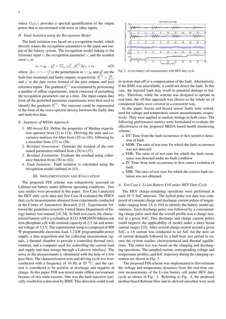
The HEV charge-sustaining operations were performed ateach 10 % SoC intervals. The hybrid pulse test data was com-posed of constant charge and discharge current pulses of magni-tudes ranging from 1A to 10A to identify the battery model pa-rameters. Each discharge pulse was followed by a correspond-ing charge pulse such that the overall profile was a charge neu-tral at a given SoC. This discharge and charge current pulsescould improve the applicability of model under a more broadcurrent ranges [15]. After several charge neutral around a givenSoC, a 1A current was conducted to set SoC for the next setof current demands followed by a half-hour rest period to en-sure the system reaches electrochemical and thermal equilib-rium. The entire test was based on the charging and discharg-ing operations. The sampled current, corresponding voltage andtemperature profiles, and SoC trajectory during the charging op-eration are shown in Fig. 3.

The proposed FDI scheme was implemented to first estimatethe voltage and temperature dynamics from the real-time cur-rent measurements of the Li-ion battery cell under HEV dutycycle as shown in Fig. 3. Referring to Fig. 4, the proposedmedian-based Kalman filter and its derived smoother were used

7

TABLE IPERFORMANCE EVALUATION OF FAULTS IN HEV1

Metric DTEKF DTMKF DTMKS MDREKF MDRMKF MDRMKS FDREKF FDRMKF FDRMKS IT MIR

∆VHEV 28.403 19.036 19.247 0 0 0 0.046 0.069 0.024 19.330 0.304

∆THEV 24.536 16.229 20.132 0 0 0 0.045 0.027 0.022 10.527 0.114

1In this table, ∆V and ∆T are the voltage and temperature faults respectively. DT is the detection time, MDR is the missed detection rate, FDR is the falsedetection rate, IT is the isolation time and MIR is the missed isolation rate. Subscript EKF, MKF and MKS are the acronymns of extended Kalman filter,median-based Kalman filter and median-based Kalman smoother respectively.

0 2 4 6 8 10 12 14 16 18 202

2.25

2.5

2.75

3.0

time window (hour)

volta

ge (

V)

Extended Kalman FilterMedian−based Kalman FilterMedian−Based Kalman SmootherVoltage measurement

Fig. 4. Comparison of battery cell voltage estimates for HEV duty cycle

0 2 4 6 8 10 12 14 16 18 20

19.85

19.9

19.95

20

20.05

20.1

20.15

20.2

20.25

20.3

20.35

time window (hour)

tem

pera

ture

(0 C

)

Extended Kalman FilterMedian−based Kalman FilterMedian−Based Kalman SmootherVoltage measurement

Fig. 5. Comparison of battery cell temperature estimates for HEV duty cycle

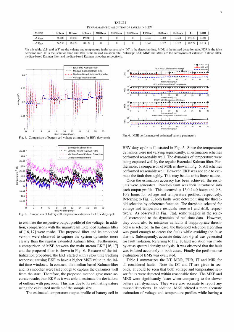
to estimate the respective output profile of the voltage. In addi-tion, comparisons with the mainstream Extended Kalman filterof [16, 17] were made. The proposed filter and its smoothedversion were observed to capture the system dynamics moreclearly than the regular extended Kalman filter. Furthermore,a comparison of MSE between the main stream EKF [16, 17]and the proposed filter is shown in Fig. 6. Because of the ini-tialization procedure, the EKF started with a slow time trackingresponse, causing EKF to have a higher MSE value in the ini-tial time windows. In contrast, the median-based Kalman filterand its smoother were fast enough to capture the dynamics wellfrom the start. Therefore, the proposed method gave more ac-curate results than EKF as it was able to estimate the deviationsof outliers with precision. This was due to its estimating natureusing the calculated median of the sample size.

The estimated temperature output profile of battery cell in

0 2 4 6 8 10 12 14 16 18 2010

−2

100

time window (hour)

MS

E

HEV: MSE Comparison of Voltage

MSE−EKF

MSE−MKF

MSE−MKS

0 2 4 6 8 10 12 14 16 18 2010

−3

10−2

10−1

time window (hour)

MS

E

HEV: MSE Comparison of Temperature

0 2 4 6 8 10 12 14 16 18 2010

−3

10−2

10−1

time window (hour)

MS

E

PHEV: MSE Comparison of Voltage

0 2 4 6 8 10 12 14 16 18 20

10−2

100

time window (hour)

MS

E

PHEV: MSE Comparison of Temperature

Fig. 6. MSE performance of estimated battery parameters

HEV duty cycle is illustrated in Fig. 5. Since the temperaturedynamics were not varying significantly, all estimation schemesperformed reasonably well. The dynamics of temperature werebeing captured well by the regular Extended Kalman filter. Fur-thermore, a comparison of MSE is shown in Fig. 6. All schemesperformed reasonably well. However, EKF was not able to esti-mate the fault thoroughly. This may be due to its linear nature.

Once the estimation accuracy has been achieved, the resid-uals were generated. Random fault was then introduced intoeach output profile. This occurred at 13.0-14.0 hours and 9.8-10.9 hours for voltage and temperature profiles, respectively.Referring to Fig. 7, both faults were detected using the thresh-old selection by coherence function. The threshold selected forvoltage and temperature residuals were ±1 and ±10, respec-tively. As observed in Fig. 7(a), some wiggles in the resid-ual correspond to the dynamics of real-time data. However,they could also be mistaken as faults if inappropriate thresh-old was selected. In this case, the threshold selection algorithmwas good enough to detect the faults while avoiding the falsealarms. Subsequently, accurate detection signal was generatedfor fault isolation. Referring to Fig. 8, fault isolation was madeby cross spectral density analysis. It was observed that the faultwas isolated accurately in both cases. Finally the performanceevaluation of BMS was evaluated.

Table I summarizes the DT, MDR, FDR, IT and MIR forall considered faults. Note the DT and IT are given in sec-onds. It could be seen that both voltage and temperature sen-sor faults were detected within reasonable time. The MKF andMKS were significantly faster when comparing to the slowerbattery cell dynamics. They were also accurate to report anymissed detections. In addition, MKS offered a more accurateestimation of voltage and temperature profiles while having a

8

0 2 4 6 8 10 12 14 16 18 20−3

−2

−1

0

1

2

time window (hour)(a)

Res

idua

l Sig

nal

0 2 4 6 8 10 12 14 16 18 20−20−10

0102030405060

time window (hour)(b)

Res

idua

l Sig

nal

Voltage ResidualVoltage Threshold

Temperature ResidualTemperature Threshold

Fig. 7. a) Battery cell voltage sensor residual in HEV duty cycle, and b)Battery cell temperature sensor residual in HEV duty cycle

0 2 4 6 8 10 12 14 16 18 20

0

1

time window (hour)

Isol

atio

n S

igna

l

Fault Isolation

0 2 4 6 8 10 12 14 16 18 20

0

1

time window (hour)

Isol

atio

n S

igna

l

Fault Isolation

Fig. 8. a) Battery cell voltage sensor fault detection in HEV duty cycle, andb) Battery cell temperature sensor fault detection in HEV duty cycle

slightly longer time than MKF. Although the isolation ratio wasquiet low for both proposed methods, there were some missedisolations. Overall, the proposed MKS took less time than thestandard EKF. Moreover, the FDR of MKS was comparativelysmaller than EKF.

B. Test Case II: Li-ion Battery Cell under PHEV Duty Cycle

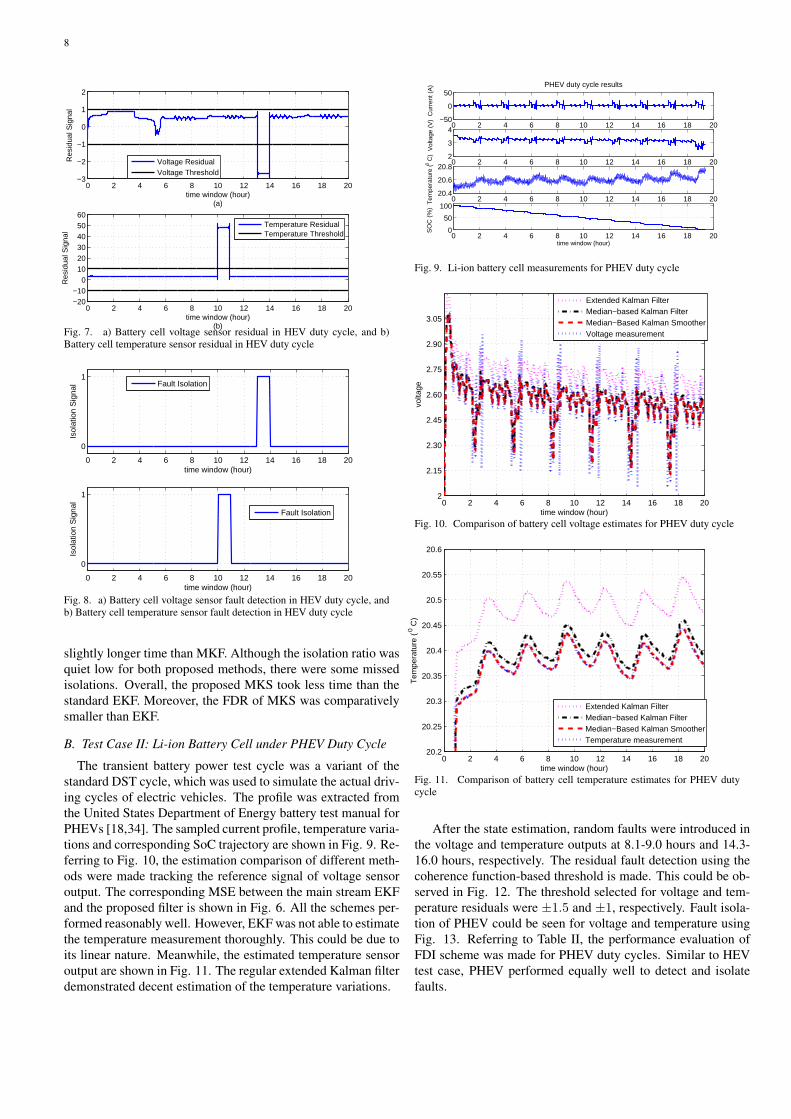
The transient battery power test cycle was a variant of thestandard DST cycle, which was used to simulate the actual driv-ing cycles of electric vehicles. The profile was extracted fromthe United States Department of Energy battery test manual forPHEVs [18,34]. The sampled current profile, temperature varia-tions and corresponding SoC trajectory are shown in Fig. 9. Re-ferring to Fig. 10, the estimation comparison of different meth-ods were made tracking the reference signal of voltage sensoroutput. The corresponding MSE between the main stream EKFand the proposed filter is shown in Fig. 6. All the schemes per-formed reasonably well. However, EKF was not able to estimatethe temperature measurement thoroughly. This could be due toits linear nature. Meanwhile, the estimated temperature sensoroutput are shown in Fig. 11. The regular extended Kalman filterdemonstrated decent estimation of the temperature variations.

0 2 4 6 8 10 12 14 16 18 20−50

0

50PHEV duty cycle results

Cur

rent

(A

)

0 2 4 6 8 10 12 14 16 18 202

3

4

Vol

tage

(V

)

0 2 4 6 8 10 12 14 16 18 2020.4

20.6

20.8

Tem

pera

ture

(0 C)

0 2 4 6 8 10 12 14 16 18 200

50

100

time window (hour)

SO

C (

%)

Fig. 9. Li-ion battery cell measurements for PHEV duty cycle

0 2 4 6 8 10 12 14 16 18 202

2.15

2.30

2.45

2.60

2.75

2.90

3.05

time window (hour)

volta

ge

Extended Kalman FilterMedian−based Kalman FilterMedian−Based Kalman SmootherVoltage measurement

Fig. 10. Comparison of battery cell voltage estimates for PHEV duty cycle

0 2 4 6 8 10 12 14 16 18 2020.2

20.25

20.3

20.35

20.4

20.45

20.5

20.55

20.6

time window (hour)

Tem

pera

ture

( 0 C

)

Extended Kalman FilterMedian−based Kalman FilterMedian−Based Kalman SmootherTemperature measurement

Fig. 11. Comparison of battery cell temperature estimates for PHEV dutycycle

After the state estimation, random faults were introduced inthe voltage and temperature outputs at 8.1-9.0 hours and 14.3-16.0 hours, respectively. The residual fault detection using thecoherence function-based threshold is made. This could be ob-served in Fig. 12. The threshold selected for voltage and tem-perature residuals were ±1.5 and ±1, respectively. Fault isola-tion of PHEV could be seen for voltage and temperature usingFig. 13. Referring to Table II, the performance evaluation ofFDI scheme was made for PHEV duty cycles. Similar to HEVtest case, PHEV performed equally well to detect and isolatefaults.

9

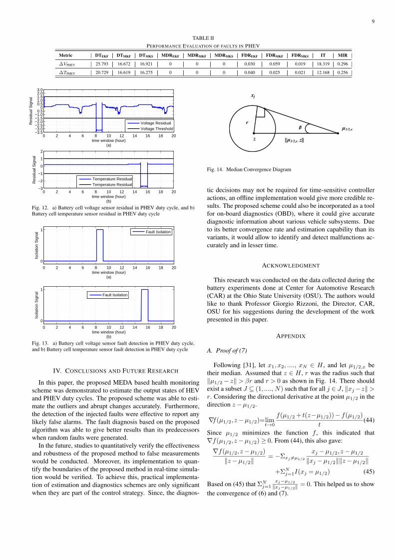
TABLE IIPERFORMANCE EVALUATION OF FAULTS IN PHEV

Metric DTEKF DTMKF DTMKS MDREKF MDRMKF MDRMKS FDREKF FDRMKF FDRMKS IT MIR

∆VPHEV 25.793 16.672 16.921 0 0 0 0.030 0.059 0.019 18.319 0.296

∆TPHEV 20.729 16.619 16.275 0 0 0 0.040 0.025 0.021 12.168 0.256

0 2 4 6 8 10 12 14 16 18 20−3.5−3.0−2.5−2.0−1.5−1.0

0.50

0.51.01.52.03.0

time window (hour)(a)

Res

idua

l Sig

nal

0 2 4 6 8 10 12 14 16 18 20−3

−2

−1

0

1

2

time window (hour)(b)

Res

idua

l Sig

nal

Voltage ResidualVoltage Threshold

Temperature ResidualTemperature Residual

Fig. 12. a) Battery cell voltage sensor residual in PHEV duty cycle, and b)Battery cell temperature sensor residual in PHEV duty cycle

0 2 4 6 8 10 12 14 16 18 20

0

1

time window (hour)(a)

Isol

atio

n S

igna

l

Fault Isolation

0 2 4 6 8 10 12 14 16 18 20

0

1

time window (hour)(b)

Isol

atio

n S

igna

l

Fault Isolation

Fig. 13. a) Battery cell voltage sensor fault detection in PHEV duty cycle,and b) Battery cell temperature sensor fault detection in PHEV duty cycle

IV. CONCLUSIONS AND FUTURE RESEARCH

In this paper, the proposed MEDA based health monitoringscheme was demonstrated to estimate the output states of HEVand PHEV duty cycles. The proposed scheme was able to esti-mate the outliers and abrupt changes accurately. Furthermore,the detection of the injected faults were effective to report anylikely false alarms. The fault diagnosis based on the proposedalgorithm was able to give better results than its predecessorswhen random faults were generated.

In the future, studies to quantitatively verify the effectivenessand robustness of the proposed method to false measurementswould be conducted. Moreover, its implementation to quan-tify the boundaries of the proposed method in real-time simula-tion would be verified. To achieve this, practical implementa-tion of estimation and diagnostics schemes are only significantwhen they are part of the control strategy. Since, the diagnos-

Fig. 14. Median Convergence Diagram

tic decisions may not be required for time-sensitive controlleractions, an offline implementation would give more credible re-sults. The proposed scheme could also be incorporated as a toolfor on-board diagnostics (OBD), where it could give accuratediagnostic information about various vehicle subsystems. Dueto its better convergence rate and estimation capability than itsvariants, it would allow to identify and detect malfunctions ac-curately and in lesser time.

ACKNOWLEDGMENT

This research was conducted on the data collected during thebattery experiments done at Center for Automotive Research(CAR) at the Ohio State University (OSU). The authors wouldlike to thank Professor Giorgio Rizzoni, the Director, CAR,OSU for his suggestions during the development of the workpresented in this paper.

APPENDIX

A. Proof of (7)

Following [31], let x1, x2, ...., xN ∈ H , and let µ1/2,x betheir median. Assumed that z ∈ H , r was the radius such that∥µ1/2 − z∥ > βr and r > 0 as shown in Fig. 14. There shouldexist a subset J ⊆ (1, ...., N) such that for all j ∈ J , ∥xj−z∥>r. Considering the directional derivative at the point µ1/2 in thedirection z−µ1/2.

∇f(µ1/2,z−µ1/2)=limt→0

f(µ1/2 + t(z−µ1/2))− f(µ1/2)

t(44)

Since µ1/2 minimizes the function f , this indicated that∇f(µ1/2,z−µ1/2)≥ 0. From (44), this also gave:

∇f(µ1/2,z−µ1/2)

∥z−µ1/2∥= −Σxj =µ1/2

xj −µ1/2,z−µ1/2

∥xj −µ1/2∥∥z−µ1/2∥+ΣN

j=1I(xj = µ1/2) (45)

Based on (45) that ΣNj=1

xj−µ1/2

∥xj−µ1/2∥= 0. This helped us to show

the convergence of (6) and (7).

10

B. Proof of Properties of Theorem II.1

Proof of Property 1:argmin

s∈HΣN

i=1 ∥ xi − s ∥= IEµ1/2(X)

argmins∈H

ΣNi=1 ∥ cxi − s ∥= argmin

sc

ΣNi=1 ∥ cxi −

s

c∥

= mins∈cH

ΣNi=1 ∥ cxi − s ∥, cH : ch : h ∈H

ΣNi=1 ∥ cxi − cIEµ1/2

(x) ∥= |c|ΣNi=1 ∥ xi − IEµ1/2

(x) ∥= |c|argmin

s∈HΣN

i=1 ∥ xi − s ∥= argmins∈H

ΣNi=1 ∥ cxi − cs ∥

= arg minsc∈H

ΣNi=1 ∥ cxi − s ∥,wheres=

s

c

= mins∈cH

ΣNi=1 ∥ cxi − s ∥=ΣN

i=1 ∥ cxi − IEµ1/2(x) ∥

= mins∈H

ΣNi=1 ∥ cxi − s ∥ (46)

where cH =H since H is a linear operator..Proof of Property 2:= argmin

s∈HΣN

i=1 ∥ axi + byi − s ∥

≤ ΣNi=1 ∥ axi + byi + aIEµ1/2

(x)+ bIEµ1/2(y) ∥

≤ ΣNi=1(∥ axi + aIEµ1/2

(x) ∥+ ∥ byi + bIEµ1/2(y) ∥)

= ΣNi=1 ∥ axi + aIEµ1/2

(x) ∥+ΣNi=1 ∥ byi + bIEµ1/2

(y) ∥= min

s∈HΣN

i=1 ∥ axi − s ∥+mins∈H

ΣNi=1 ∥ byi − s ∥

≤ mins∈H

ΣNi=1(∥ axi − s ∥∥ byi − s ∥) (47)

Proof of Property 3: It follows the proof of Property 2.Property 4: If X was an independent variable, then for the

higher moments of X , i.e. IEµ1/2[X2],

IEµ1/2[X2] = IEµ1/2

[(X − IEµ1/2[X])2]

= argminθ1

|[X − argminθ2

|X − θ2|]2 − θ1|

= argminθ1

|X2 − 2X(argminθ2

|X − θ2|)

+ (argminθ2

|X − θ2|)2 − θ1| (48)

where θ1 and θ2 represents the expectation IEµ1/2,1 and IEµ1/2,2

respectively.

C. Proof of theorem II.2:

Consider the following Lyapunov function,

V (et) = e∗x,tPtex,t (49)

where Pt was defined as the solution of (30), Qt was chosensuch that ρ1 = λmin(Qt)− 2∥Ht∥.|Rt|ξf,tL0 > 0. Along thetrajectory of the fault-free system, the corresponding Lyapunovdifference along the trajectory et could be expressed as:

∆V = IEV (et+1|et,Pt)−V (et)

= IEe∗t+1Ptet+1− e∗tPtet

= (Ae,tex,t +BL0,tue,t)∗Pt(Ae,tex,t +BL0,tue,t)

−e∗x,tPtex,t

= e∗t [(Pt(At −KtHt)+ (At −KtHt)∗Pt)

+PtBtξf,t[(ut,zt,xt)− (ut,zt, xt)]]et (50)

From Assumption II.2 and system described by (30), one couldfurther claim:

∆V ≤ −eTx,tQtex,t +2∥ez,t∥.|Rit|ξf,tL0∥ex,t∥

≤ −ρ1∥ex,t∥2 < 0 (51)

Thus, limt→∞ ex,t = 0 and limt→∞ez,t = 0. This completedthe proof.

REFERENCES

[1] H. Budde-Meiwes, J. Drillkens, B. Lunz, J. Muennix, S. Rothgang, J.Kowal, and D. U. Sauer, “A review of current automotive battery technol-ogy and future prospects,” Jour. Auto. Engg., vol. 227, no. 5, pp. 761–776,2013.

[2] A. Burke and M. Miller, “Performance characteristics of lithium-ion bat-teries of various chemistries for plug-in hybrid vehicles,” EVS24 Intl. Bat-tery, Hybrid and Fuel Cell Elec. Vehicle Symp., Stavanger, Norway, pp.1–13, May 2009.

[3] A. Dinger, R. Martin, X. Mosquet, M. Rabl, D. Rizoulis, M. Russo, andG. Sticher, “Batteries for electric cars: Challenges, opportunities, and theoutlook to 2020,” tech. rep., The Boston Consulting Group, 2010.

[4] M. Lowe, S. Tokuoka, T. Trigg, and G. Gereffi, “Lithium-ion batteries forelectric vehicles,” tech. rep., Center of Glob., Governance & Competitive-ness, Duke Uni., Oct. 5, 2010.

[5] L. G. Lu, X. B. Han, J. Q. Li, J. F. Hua, and M. G. Ouyang, “A review onthe key issues for lithium-ion battery management in electric vehicles,” J.Power Sour., vol. 226, pp. 272-288, Mar. 2013.

[6] P. Arora, R. E. White, and M. Doyle, “Capacity fade mechanisms and sidereactions in lithium-ion batteries,” J. Electrochem. Soc., vol. 145, no. 10,pp. 3647-3667, Apr. 1998.

[7] L. Lu, X. Han, J. Li, J. Hua, and M. Ouyang, “A review on the key issuesfor lithium-ion battery management in electric vehicles,” J. Power Sour.,vol. 226, pp. 272–288, 2013.

[8] K. Zaghib, M. Dontigny, “Safe and fast-charging Li-ion battery with longshelf life for power applications,” J. Power Sour. vol. 196, pp. 3949–3954,2011.

[9] X. Han, M. Ouyang, L. Lu, J. Li, Y. Zheng, and Z. Li, “A comparativestudy of commercial lithium-ion battery cycle life in electrical vehicle:Aging mechanism identification,” J. Power Sour., vol. 251, pp. 38–54,2013.

[10] D. P. Abraham, E. P. Roth, R. Kostecki, K. McCarthy, S. MacLaren, S.,and D. H. Doughty, “Diagnostic examination of thermally abused high-power lithium-ion cells,” J. Power Sour., vol. 161, no. 1, pp. 648-657,Oct. 2006.

[11] Q. S. Wang, P. Ping, X. J. Zhao, G. Q. Chu, J. H. Sun, and C. H. Chen,“Thermal runaway caused fire and explosion of lithium-ion battery,” J.Power Sour., vol. 208, pp. 210-224, Jun. 2012.

[12] C. Mikolajczak, M. Kahn, K. White, K., and R. T. Long, R.T. “Lithium-ion batteries hazard and use assessment,” Fin. Rprt. Fire Protect. Res.Foun., Jul. 2011.

[13] H. D. Daniel, and A. P. Ahmad, “Vehicle battery safety roadmap guid-ance,” Battery Safety Consulting (subcontractor), NREL Report No.SR-5400-54404, Oct. 2012.

[14] Z. Liu, Q. Ahmed, G. Rizzoni, and H. He, “Fault detection and isola-tion for lithium-ion battery system using structural analysis and sequentialresidual generation,” 7th ASME Annual Dynamic Sys. and Ctrl., TX, US,2014.

[15] Y. Hu, S. Yurkovich, Y. Guezennec, and B. J. Yurkovich, “Electro-thermalbattery model identification for automotive applications,” J. Power Sour.,vol. 196, no. 1, pp. 449-457, Jan. 2011.

[16] A. Singh, A. Izadian, and S. Anwar, “Adaptive nonlinear model-basedfault diagnosis of Li-ion Batteries,” IEEE Trans. Indus. Elect., Article inPress, DOI: 10.1109/TIE.2014.2336599, Jul. 2014.

[17] H. He, R. Xiong, X. Zhang, F. Sun, and J. Fan, “State-of-Charge estima-tion of the lithium-ion battery using an adaptive extended Kalman filterbased on an improved Thevenin model,” IEEE Trans. Vehi. Tech., vol. 60,no. 4, pp. 1461–1469, May 2011.

[18] J. Marcicki, M. Canova, M., A. T. Conlisk, and G. Rizzoni, “Designand parametrization analysis of a reduced-order electrochemical model ofgraphite/LiFePO4 cells for SOC/SOH estimation,” Jour. Power Sour.,vol. 237, pp, 310-324, Sep. 2013.

[19] S. F. Schmidt, “The Kalman filter: Its recognition and development foraerospace applications,” AIAA J. Guid. Contr., vol. 4, pp. 4–7, 1981.

11

[20] M. S. Grewal, V. Henderson, V., and R. Miyasako, R., “Application ofKalman filtering to the calibration and alignment of inertial navigationsystems,” IEEE Trans. Automat. Contr., vol. 36, no. 1, pp. 4–14, Jan. 1991.

[21] Grewal, M. S., Weill, L. R., and Andrews, A. P., “Global positioning sys-tems, inertial navigation, and integration,” 2nd ed. Hoboken, NJ: Wiley,2007.

[22] E. Kaplan, E., and C. Hegarty, “Understanding GPS: Principles and appli-cations, Second Edition,” Norwell, MA, USA: Artech House, 2005.

[23] H. Hijazi, and L. Ros, “Joint data QR-detection and Kalman estimationfor OFDM time-varying Rayleigh channel complex gains,” IEEE Trans.Commun., vol. 58, no. 1, pp. 170–178, Jan. 2010.

[24] C. Komninakis, C. Fragouli, A. Sayed, and R. Wesel, “Multi-input multi-output fading channel tracking and equalization using Kalman estima-tion,” IEEE Trans. Sig. Process., vol. 50, no. 5, pp. 1065–1076, May 2002.

[25] H. M. Khalid and J. C.-H. Peng, “Improved recursive electromechani-cal oscillations monitoring scheme: A novel distributed approach,” IEEETrans. Pow. Syst., vol. 30, no. 2, pp. 680–688, Mar. 2015.

[26] B. S. Everitt, “The Cambridge dictionary of statistics,” Cambridge Uni-versity Press, Cambridge.

[27] H. Cardot, P. Cenac, P., and M. Chaouch, “Stochastic approximation to themultivariate and the functional median,” Compstat 2010, Physica Verlag,Springer, pp. 421–428, 2010.

[28] C. Mallows, “Another comment on O’Cinneide,” The American Statisti-cian, vol. 45, no. 3, pp. 257, Aug. 1991.

[29] S. Stigler, “Studies in the history of probability and statistics XXXII:Laplace, Fisher and the discovery of the concept of sufficiency,”Biometrika, vol. 60, no. 3, pp. 439–445, Dec. 1973.

[30] R. Faragher, “Understanding the basis of the Kalman filter via a simpleand intuitive derivation,” IEEE Sig. Process. Mag., pp. 128–132, Aug.2012.

[31] M. Stanislav, “Geometric median and robust estimation in banach spaces,”pp. 1–28, arXiv: math.ST/1308.1334.

[32] T. Yanagisawa, H. Takayama, “Coherence coefficient measuring systemand its application to some acoustic measurements,” Applied Acoustics,vol. 16, no. 2, pp. 105–119, Mar. 1983.

[33] C. Zheng, H. Yang, and X. Li, “On generalized auto-spectral coherencefunction and its applications to signal detection,” IEEE Sig. Process. let.,vol. 21, no. 5, pp. 559–563, May 2014.

[34] “Battery test manual for Plug-In hybrid electric vehicles,” U.S. Dept. Ener.Vehicle Tech. Program, Revision 0, Mar. 2008.

Haris M. Khalid (M’13) received his M.S and Ph.D.degrees from King Fahd University of Petroleum andMinerals (KFUPM), Dhahran, Kingdom of Saudi Ara-bia, in 2009 and 2012, respectively. He has workedas a research fellow at Distributed Control ResearchGroup at KFUPM. Since 2013, he has been working asa Postdoctoral Researcher with Department of Electri-cal Engineering and Computer Science at Masdar Insti-tute of Science and Technology (MI) collaborated withMI-MIT Cooperative Program. His research interestsare power systems, signal processing, fault diagnostics,

filtering, estimation, performance monitoring and battery management systems.

Qadeer Ahmed (M’11) received the B.S. degree inmechatronics and control engineering from the Uni-versity of Engineering and Technology, Lahore, Pak-istan, in 2007 and the M.S. and PhD degree in con-trol systems from Mohammad Ali Jinnah University,Islamabad, Pakistan, in 2009 and 2011. He is currentlySenior Research Associate at The Ohio State Univer-sity, Center for Automotive Research. He is workingon next generation of energy efficient vehicle power-trains. He has authored more than 33 international pub-lications. His research interests include modeling, esti-

mation, control and diagnostics of automotive systems.

Jimmy C. -H. Peng (S’05-M’12) received the B.E.(Hons.) and Ph.D. degrees from the University ofAuckland, Auckland, New Zealand, in 2008 and 2012,respectively. In 2012, he joined the Department ofElectrical Engineering and Computer Science at Mas-dar Institute of Science and Technology, Abu Dhabi,United Arab Emirates, as an Assistant Professor ofElectrical Power Engineering. He was a Visiting Scien-tist with the Research Laboratory of Electronics (RLE)and a Visiting Assistant Professor with the MIT-MI Co-operative Program at Massachusetts Institute of Tech-

nology (MIT), in 2013 and 2014, respectively. His research interests are powersystem stability, synchrophasor measurements, real-time system identification,and high performance computing.