1 fall 2004, cis, temple university cis527: data warehousing, filtering, and mining lecture 6...
TRANSCRIPT

1
Fall 2004, CIS, Temple University
CIS527: Data Warehousing, Filtering, and Mining
Lecture 6
• Clustering
Lecture slides taken/modified from:– Jiawei Han (http://www-sal.cs.uiuc.edu/~hanj/DM_Book.html)– Vipin Kumar (http://www-users.cs.umn.edu/~kumar/csci5980/index.html)

3
General Applications of Clustering
• Pattern Recognition• Spatial Data Analysis
– create thematic maps in GIS by clustering feature spaces
– detect spatial clusters and explain them in spatial data mining
• Image Processing• Economic Science (especially market research)• WWW
– Document classification– Cluster Weblog data to discover groups of similar
access patterns

4
Examples of Clustering Applications
• Marketing: Help marketers discover distinct groups in their customer bases, and then use this knowledge to develop targeted marketing programs
• Land use: Identification of areas of similar land use in an earth observation database
• Insurance: Identifying groups of motor insurance policy holders with a high average claim cost
• City-planning: Identifying groups of houses according to their house type, value, and geographical location
• Earth-quake studies: Observed earth quake epicenters should be clustered along continent faults

5
What Is Good Clustering?
• A good clustering method will produce high quality
clusters with– high intra-class similarity
– low inter-class similarity
• The quality of a clustering result depends on both the
similarity measure used by the method and its
implementation.
• The quality of a clustering method is also measured by its
ability to discover some or all of the hidden patterns.

6
Requirements of Clustering in Data Mining
• Scalability
• Ability to deal with different types of attributes
• Discovery of clusters with arbitrary shape
• Minimal requirements for domain knowledge to determine input parameters
• Able to deal with noise and outliers
• Insensitive to order of input records
• High dimensionality
• Incorporation of user-specified constraints
• Interpretability and usability
7
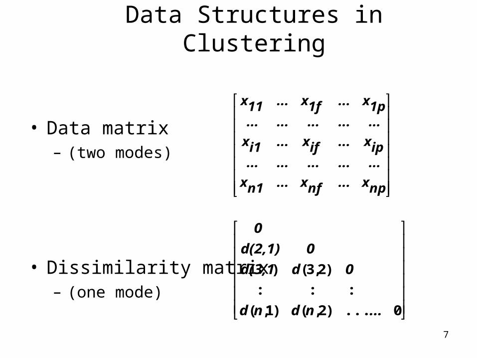
Data Structures in Clustering
• Data matrix– (two modes)
• Dissimilarity matrix– (one mode)
npx...nfx...n1x
...............ipx...ifx...i1x
...............1px...1fx...11x
0...)2,()1,(
:::
)2,3()
...ndnd
0dd(3,1
0d(2,1)
0

8
Measuring Similarity
• Dissimilarity/Similarity metric: Similarity is expressed in terms of a distance function, which is typically metric:
d(i, j)• There is a separate “quality” function that measures the
“goodness” of a cluster.• The definitions of distance functions are usually very
different for interval-scaled, boolean, categorical, ordinal and ratio variables.
• Weights should be associated with different variables based on applications and data semantics.
• It is hard to define “similar enough” or “good enough” – the answer is typically highly subjective.

9
Interval-valued variables
• Standardize data
– Calculate the mean squared deviation:
where
– Calculate the standardized measurement (z-score)
• Using mean absolute deviation could be more robust
than using standard deviation
.)...21
1nffff
xx(xn m
)2||...2||2|(|121 fnffffff
mxmxmxns
f
fifif s
mx z

10
Similarity and Dissimilarity Between Objects
• Distances are normally used to measure the similarity or
dissimilarity between two data objects
• Some popular ones include: Minkowski distance:
where i = (xi1, xi2, …, xip) and j = (xj1, xj2, …, xjp) are two p-
dimensional data objects, and q is a positive integer
• If q = 1, d is Manhattan distance
pp
jx
ix
jx
ix
jx
ixjid )||...|||(|),(
2211
||...||||),(2211 pp jxixjxixjxixjid
11
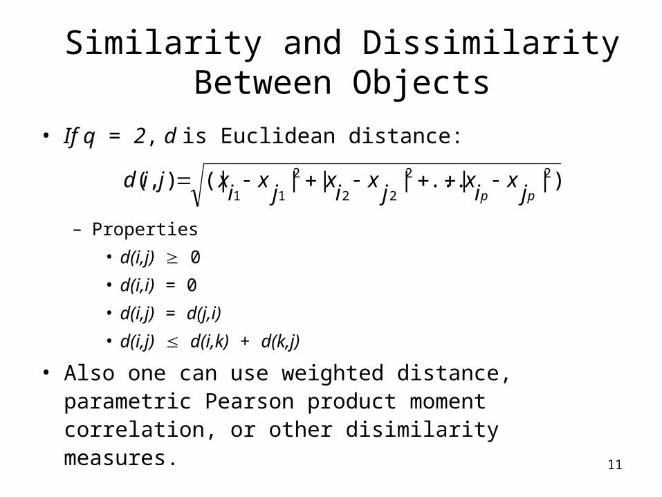
• If q = 2, d is Euclidean distance:
– Properties
• d(i,j) 0
• d(i,i) = 0
• d(i,j) = d(j,i)
• d(i,j) d(i,k) + d(k,j)
• Also one can use weighted distance, parametric Pearson product moment correlation, or other disimilarity measures.
)||...|||(|),( 22
22
2
11 pp jx
ix
jx
ix
jx
ixjid
Similarity and Dissimilarity Between Objects

12
Mahalanobis Distance
Tqpqpqpsmahalanobi )()(),( 1
For red points, the Euclidean distance is 14.7, Mahalanobis distance is 6.
is the covariance matrix of the input data X
n
i
kikjijkj XXXXn 1
, ))((1
1
13
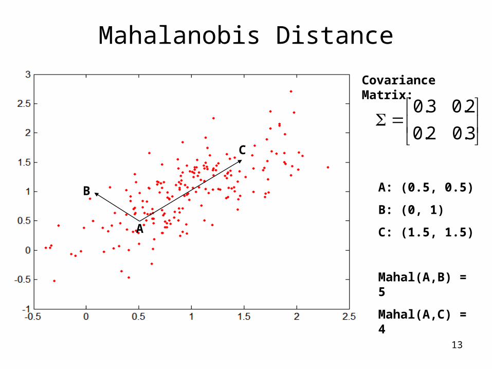
Mahalanobis Distance
Covariance Matrix:
3.02.0
2.03.0
B
A
C
A: (0.5, 0.5)
B: (0, 1)
C: (1.5, 1.5)
Mahal(A,B) = 5
Mahal(A,C) = 4

14
Cosine Similarity
• If d1 and d2 are two document vectors, then
cos( d1, d2 ) = (d1 d2) / ||d1|| ||d2|| , where indicates vector dot product and || d || is the length of vector d.
• Example:
d1 = 3 2 0 5 0 0 0 2 0 0
d2 = 1 0 0 0 0 0 0 1 0 2
d1 d2= 3*1 + 2*0 + 0*0 + 5*0 + 0*0 + 0*0 + 0*0 + 2*1 + 0*0 + 0*2 = 5
||d1|| = (3*3+2*2+0*0+5*5+0*0+0*0+0*0+2*2+0*0+0*0)0.5 = (42) 0.5 = 6.481
||d2|| = (1*1+0*0+0*0+0*0+0*0+0*0+0*0+1*1+0*0+2*2) 0.5 = (6) 0.5 = 2.245
cos( d1, d2 ) = .3150

15
Correlation Measure
Scatter plots showing the similarity from –1 to 1.

16
Binary Variables
• A contingency table for binary data
• Simple matching coefficient (invariant, if the binary variable is
symmetric):
• Jaccard coefficient (noninvariant if the binary variable is
asymmetric):
dcbacb jid
),(
pdbcasum
dcdc
baba
sum
0
1
01
cbacb jid
),(
Object i
Object j

17
Dissimilarity between Binary Variables
• Example
– gender is a symmetric attribute– the remaining attributes are asymmetric binary– let the values Y and P be set to 1, and the value N be set to 0
Name Gender Fever Cough Test-1 Test-2 Test-3 Test-4
Jack M Y N P N N NMary F Y N P N P NJim M Y P N N N N
75.0211
21),(
67.0111
11),(
33.0102
10),(
maryjimd
jimjackd
maryjackd

18
Nominal Variables
• A generalization of the binary variable in that it can take
more than 2 states, e.g., red, yellow, blue, green
• Method 1: Simple matching– m: # of matches, p: total # of variables
• Method 2: use a large number of binary variables– creating a new binary variable for each of the M nominal states
pmpjid ),(

19
Ordinal Variables
• An ordinal variable can be discrete or continuous
• order is important, e.g., rank
• Can be treated like interval-scaled – replacing xif by their rank
– map the range of each variable onto [0, 1] by replacing i-th object in the f-th variable by
– compute the dissimilarity using methods for interval-scaled variables
11
f
ifif M
rz
},...,1{fif
Mr

20
Ratio-Scaled Variables
• Ratio-scaled variable: a positive measurement on a
nonlinear scale, approximately at exponential scale,
such as AeBt or Ae-Bt
• Methods:– treat them like interval-scaled variables — not a good choice!
(why?)
– apply logarithmic transformation
yif = log(xif)
– treat them as continuous ordinal data treat their rank as interval-
scaled.

21
Variables of Mixed Types
• A database may contain all the six types of variables– symmetric binary, asymmetric binary, nominal, ordinal, interval and
ratio.
• One may use a weighted formula to combine their effects.
– f is binary or nominal:
dij(f) = 0 if xif = xjf , or dij
(f) = 1 o.w.
– f is interval-based: use the normalized distance– f is ordinal or ratio-scaled
• compute ranks rif and
• and treat zif as interval-scaled
)(1
)()(1),(
fij
pf
fij
fij
pf
djid
1
1
f
if
Mrz
if

22
Notion of a Cluster can be Ambiguous
How many clusters?
Four Clusters Two Clusters
Six Clusters
23
Other Distinctions Between Sets of Clusters
• Exclusive versus non-exclusive– In non-exclusive clusterings, points may belong to multiple
clusters.– Can represent multiple classes or ‘border’ points
• Fuzzy versus non-fuzzy– In fuzzy clustering, a point belongs to every cluster with some
weight between 0 and 1– Weights must sum to 1– Probabilistic clustering has similar characteristics
• Partial versus complete– In some cases, we only want to cluster some of the data
• Heterogeneous versus homogeneous– Cluster of widely different sizes, shapes, and densities

24
Types of Clusters
• Well-separated clusters
• Center-based clusters
• Contiguous clusters
• Density-based clusters
• Property or Conceptual
• Described by an Objective Function
25
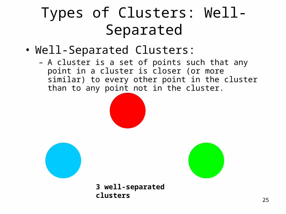
Types of Clusters: Well-Separated
• Well-Separated Clusters: – A cluster is a set of points such that any point in a cluster is
closer (or more similar) to every other point in the cluster than to any point not in the cluster.
3 well-separated clusters

26
Types of Clusters: Center-Based
• Center-based– A cluster is a set of objects such that an object in a cluster is
closer (more similar) to the “center” of a cluster, than to the center of any other cluster
– The center of a cluster is often a centroid, the average of all the points in the cluster, or a medoid, the most “representative” point of a cluster
4 center-based clusters

27
Types of Clusters: Contiguity-Based
• Contiguous Cluster (Nearest neighbor or Transitive)– A cluster is a set of points such that a point in a cluster is
closer (or more similar) to one or more other points in the cluster than to any point not in the cluster.
8 contiguous clusters

28
Types of Clusters: Density-Based
• Density-based– A cluster is a dense region of points, which is separated by
low-density regions, from other regions of high density. – Used when the clusters are irregular or intertwined, and when
noise and outliers are present.
6 density-based clusters

29
Types of Clusters: Conceptual Clusters
• Shared Property or Conceptual Clusters– Finds clusters that share some common property or represent
a particular concept. .
2 Overlapping Circles

30
Major Clustering Approaches
• Partitioning algorithms: Construct various partitions and
then evaluate them by some criterion
• Hierarchy algorithms: Create a hierarchical decomposition
of the set of data (or objects) using some criterion
• Density-based: based on connectivity and density functions
• Grid-based: based on a multiple-level granularity structure
• Model-based: A model is hypothesized for each of the
clusters and the idea is to find the best fit of that model to
each other

31
K-means Clustering
• Partitional clustering approach • Each cluster is associated with a centroid (center point) • Each point is assigned to the cluster with the closest centroid• Number of clusters, K, must be specified• The basic algorithm is very simple

32
K-means Clustering – Details• Initial centroids are often chosen randomly.
– Clusters produced vary from one run to another.
• The centroid is (typically) the mean of the points in the cluster.• ‘Closeness’ is measured by Euclidean distance, cosine similarity, correlation, etc.• K-means will converge for common similarity measures mentioned above.• Most of the convergence happens in the first few iterations.
– Often the stopping condition is changed to ‘Until relatively few points change clusters’
• Complexity is O( n * K * I * d )– n = number of points, K = number of clusters,
I = number of iterations, d = number of attributes
33
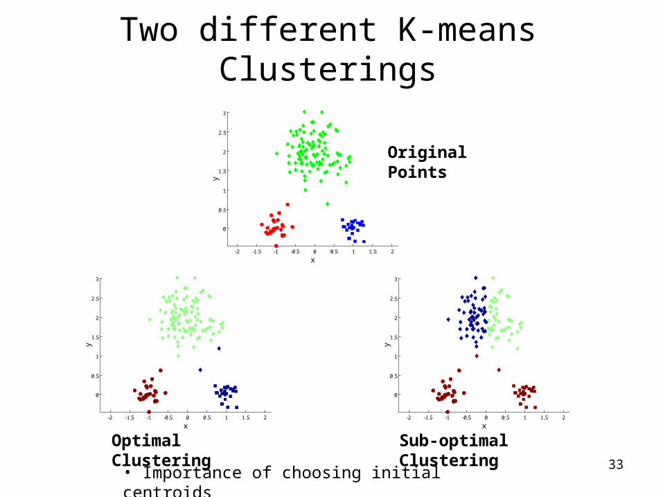
Two different K-means Clusterings
-2 -1.5 -1 -0.5 0 0.5 1 1.5 2
0
0.5
1
1.5
2
2.5
3
x
y
-2 -1.5 -1 -0.5 0 0.5 1 1.5 2
0
0.5
1
1.5
2
2.5
3
x
y
Sub-optimal Clustering
-2 -1.5 -1 -0.5 0 0.5 1 1.5 2
0
0.5
1
1.5
2
2.5
3
x
y
Optimal Clustering
Original Points
• Importance of choosing initial centroids

34
Evaluating K-means Clusters
• Most common measure is Sum of Squared Error (SSE)– For each point, the error is the distance to the nearest cluster– To get SSE, we square these errors and sum them.
– x is a data point in cluster Ci and mi is the representative point for cluster Ci
• can show that mi corresponds to the center (mean) of the cluster
– Given two clusters, we can choose the one with the smallest error– One easy way to reduce SSE is to increase K, the number of
clusters• A good clustering with smaller K can have a lower SSE than a poor
clustering with higher K
K
i Cxi
i
xmdistSSE1
2 ),(

35
Solutions to Initial Centroids Problem
• Multiple runs– Helps, but probability is not on your side
• Sample and use hierarchical clustering to determine initial centroids
• Select more than k initial centroids and then select among these initial centroids– Select most widely separated
• Postprocessing• Bisecting K-means
– Not as susceptible to initialization issues
36
Handling Empty Clusters
• Basic K-means algorithm can yield empty clusters
• Several strategies– Choose the point that contributes most to SSE– Choose a point from the cluster with the highest SSE– If there are several empty clusters, the above can be
repeated several times.

37
Pre-processing and Post-processing
• Pre-processing– Normalize the data
– Eliminate outliers
• Post-processing– Eliminate small clusters that may represent outliers
– Split ‘loose’ clusters, i.e., clusters with relatively high SSE
– Merge clusters that are ‘close’ and that have relatively low SSE
– Can use these steps during the clustering process• ISODATA

38
Bisecting K-means
• Bisecting K-means algorithm– Variant of K-means that can produce a partitional or a hierarchical clustering

39
Bisecting K-means Example

40
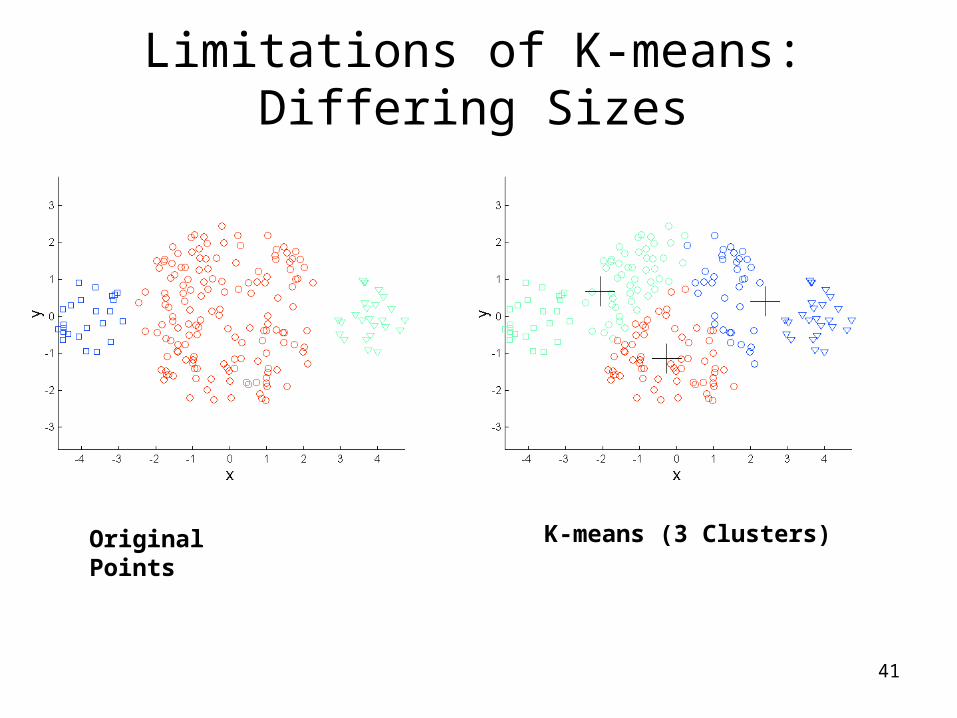
Limitations of K-means
• K-means has problems when clusters are of differing – Sizes– Densities– Non-globular shapes
• K-means has problems when the data contains outliers.
41
Limitations of K-means: Differing Sizes
Original Points K-means (3 Clusters)

42
Limitations of K-means: Differing Density
Original Points K-means (3 Clusters)

43
Limitations of K-means: Non-globular Shapes
Original Points K-means (2 Clusters)

44
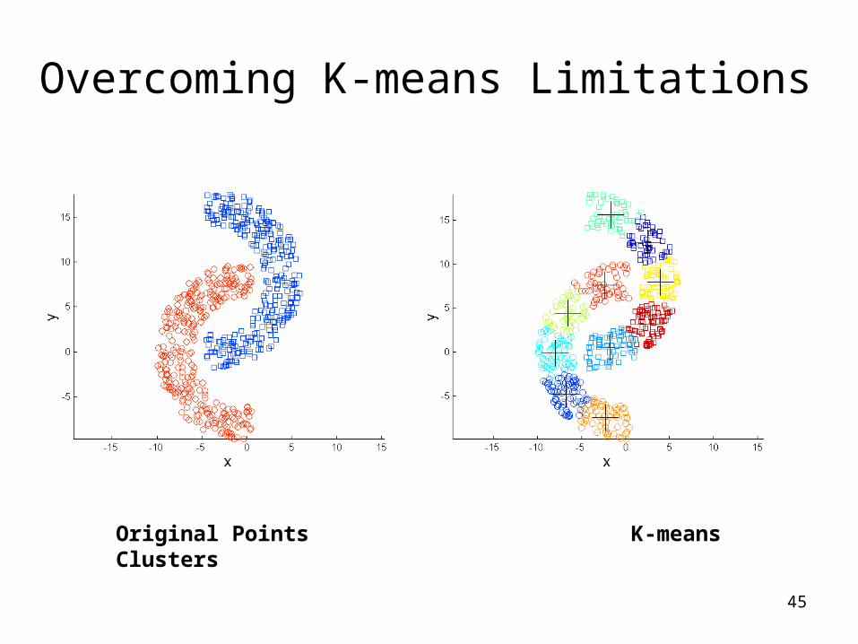
Overcoming K-means Limitations
Original Points K-means Clusters
One solution is to use many clusters.Find parts of clusters, but need to put together.
45
Overcoming K-means Limitations
Original Points K-means Clusters

46
Variations of the K-Means Method
• A few variants of the k-means which differ in– Selection of the initial k means– Dissimilarity calculations– Strategies to calculate cluster means
• Handling categorical data: k-modes (Huang’98)– Replacing means of clusters with modes– Using new dissimilarity measures to deal with categorical objects– Using a frequency-based method to update modes of clusters
• Handling a mixture of categorical and numerical data: k-prototype method

47
The K-Medoids Clustering Method
• Find representative objects, called medoids, in clusters
• PAM (Partitioning Around Medoids, 1987)– starts from an initial set of medoids and iteratively replaces one of
the medoids by one of the non-medoids if it improves the total distance of the resulting clustering
– PAM works effectively for small data sets, but does not scale well for large data sets
• CLARA (Kaufmann & Rousseeuw, 1990)– draws multiple samples of the data set, applies PAM on each
sample, and gives the best clustering as the output
• CLARANS (Ng & Han, 1994): Randomized sampling
• Focusing + spatial data structure (Ester et al., 1995)

48
Hierarchical Clustering
• Produces a set of nested clusters organized as a hierarchical tree
• Can be visualized as a dendrogram– A tree like diagram that records the sequences of
merges or splits
1 3 2 5 4 60
0.05
0.1
0.15
0.2
1
2
3
4
5
6
1
23 4
5

49
Strengths of Hierarchical Clustering
• Do not have to assume any particular number of clusters– Any desired number of clusters can be obtained by
‘cutting’ the dendogram at the proper level
• They may correspond to meaningful taxonomies– Example in biological sciences (e.g., animal kingdom,
phylogeny reconstruction, …)

50
Hierarchical Clustering
• Two main types of hierarchical clustering– Agglomerative:
• Start with the points as individual clusters• At each step, merge the closest pair of clusters until only one cluster
(or k clusters) left
– Divisive: • Start with one, all-inclusive cluster • At each step, split a cluster until each cluster contains a point (or there
are k clusters)
• Traditional hierarchical algorithms use a similarity or distance matrix– Merge or split one cluster at a time
51
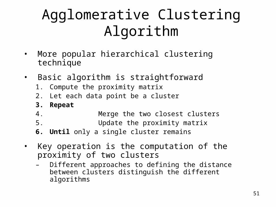
Agglomerative Clustering Algorithm
• More popular hierarchical clustering technique
• Basic algorithm is straightforward1. Compute the proximity matrix2. Let each data point be a cluster3. Repeat4. Merge the two closest clusters5. Update the proximity matrix6. Until only a single cluster remains
• Key operation is the computation of the proximity of two clusters
– Different approaches to defining the distance between clusters distinguish the different algorithms
52
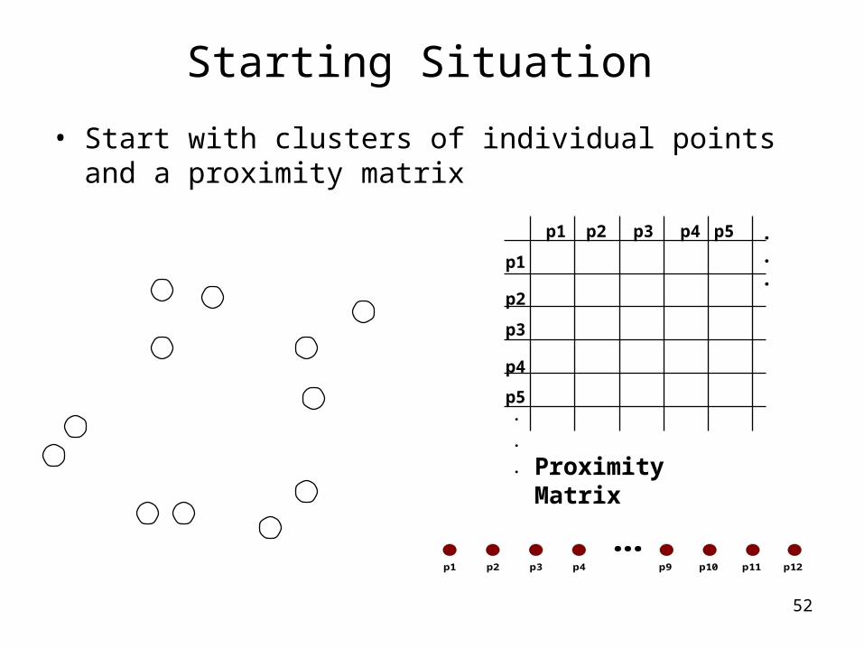
Starting Situation
• Start with clusters of individual points and a proximity matrix
p1
p3
p5
p4
p2
p1 p2 p3 p4 p5 . . .
.
.
. Proximity Matrix
...p1 p2 p3 p4 p9 p10 p11 p12

53
Intermediate Situation
• After some merging steps, we have some clusters
C1
C4
C2 C5
C3
C2C1
C1
C3
C5
C4
C2
C3 C4 C5
Proximity Matrix
...p1 p2 p3 p4 p9 p10 p11 p12
54
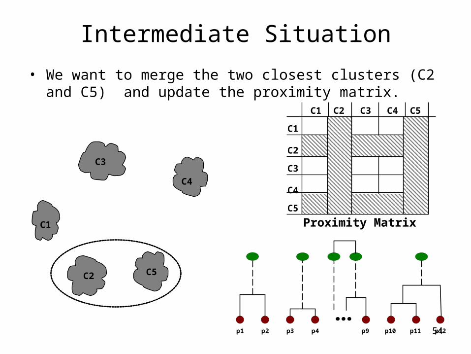
Intermediate Situation
• We want to merge the two closest clusters (C2 and C5) and update the proximity matrix.
C1
C4
C2 C5
C3
C2C1
C1
C3
C5
C4
C2
C3 C4 C5
Proximity Matrix
...p1 p2 p3 p4 p9 p10 p11 p12
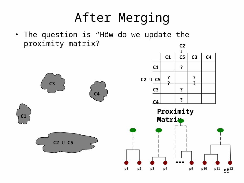
55
After Merging• The question is “How do we update the proximity matrix?”
C1
C4
C2 U C5
C3? ? ? ?
?
?
?
C2 U C5C1
C1
C3
C4
C2 U C5
C3 C4
Proximity Matrix
...p1 p2 p3 p4 p9 p10 p11 p12

56
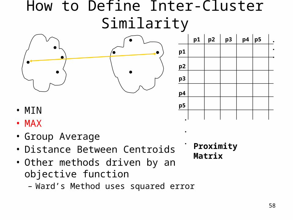
How to Define Inter-Cluster Similarity
p1
p3
p5
p4
p2
p1 p2 p3 p4 p5 . . .
.
.
.
Similarity?
• MIN• MAX• Group Average• Distance Between Centroids• Other methods driven by an
objective function– Ward’s Method uses squared error
Proximity Matrix

57
How to Define Inter-Cluster Similarity
p1
p3
p5
p4
p2
p1 p2 p3 p4 p5 . . .
.
.
.Proximity Matrix
• MIN• MAX• Group Average• Distance Between Centroids• Other methods driven by an
objective function– Ward’s Method uses squared error
58
How to Define Inter-Cluster Similarity
p1
p3
p5
p4
p2
p1 p2 p3 p4 p5 . . .
.
.
.Proximity Matrix
• MIN• MAX• Group Average• Distance Between Centroids• Other methods driven by an
objective function– Ward’s Method uses squared error

59
How to Define Inter-Cluster Similarity
p1
p3
p5
p4
p2
p1 p2 p3 p4 p5 . . .
.
.
.Proximity Matrix
• MIN• MAX• Group Average• Distance Between Centroids• Other methods driven by an
objective function– Ward’s Method uses squared error

60
How to Define Inter-Cluster Similarity
p1
p3
p5
p4
p2
p1 p2 p3 p4 p5 . . .
.
.
.Proximity Matrix
• MIN• MAX• Group Average• Distance Between Centroids• Other methods driven by an
objective function– Ward’s Method uses squared error

61
Hierarchical Clustering: Comparison
Group Average
Ward’s Method
1
2
3
4
5
61
2
5
3
4
MIN MAX
1
2
3
4
5
61
2
5
34
1
2
3
4
5
61
2 5
3
41
2
3
4
5
6
12
3
4
5

62
Hierarchical Clustering: Time and Space requirements
• O(N2) space since it uses the proximity matrix. – N is the number of points.
• O(N3) time in many cases– There are N steps and at each step the size, N2,
proximity matrix must be updated and searched– Complexity can be reduced to O(N2 log(N) ) time for
some approaches

63
Hierarchical Clustering: Problems and Limitations
• Once a decision is made to combine two clusters, it cannot be undone
• No objective function is directly minimized
• Different schemes have problems with one or more of the following:– Sensitivity to noise and outliers– Difficulty handling different sized clusters and convex
shapes– Breaking large clusters

64
MST: Divisive Hierarchical Clustering
• Build MST (Minimum Spanning Tree)– Start with a tree that consists of any point– In successive steps, look for the closest pair of points (p, q)
such that one point (p) is in the current tree but the other (q) is not
– Add q to the tree and put an edge between p and q

65
MST: Divisive Hierarchical Clustering
• Use MST for constructing hierarchy of clusters

66
More on Hierarchical Clustering Methods
• Major weakness of agglomerative clustering methods– do not scale well: time complexity of at least O(n2), where n is the
number of total objects– can never undo what was done previously
• Integration of hierarchical with distance-based clustering– BIRCH (1996): uses CF-tree and incrementally adjusts the quality
of sub-clusters– CURE (1998): selects well-scattered points from the cluster and
then shrinks them towards the center of the cluster by a specified fraction
– CHAMELEON (1999): hierarchical clustering using dynamic modeling

67
One Alternative: BIRCH
• Birch: Balanced Iterative Reducing and Clustering using Hierarchies, by Zhang, Ramakrishnan, Livny (SIGMOD’96)
• Incrementally construct a CF (Clustering Feature) tree, a hierarchical data structure for multiphase clustering
– Phase 1: scan DB to build an initial in-memory CF tree (a multi-level compression of the data that tries to preserve the inherent clustering structure of the data)
– Phase 2: use an arbitrary clustering algorithm to cluster the leaf nodes of the CF-tree
• Scales linearly: finds a good clustering with a single scan and improves the quality with a few additional scans
• Weakness: handles only numeric data, and sensitive to the order of the data record.

68
Density-Based Clustering Methods
• Clustering based on density (local cluster criterion), such as density-connected points
• Major features:– Discover clusters of arbitrary shape– Handle noise– One scan– Need density parameters as termination condition
• Several interesting studies:– DBSCAN: Ester, et al. (KDD’96)– OPTICS: Ankerst, et al (SIGMOD’99).– DENCLUE: Hinneburg & D. Keim (KDD’98)– CLIQUE: Agrawal, et al. (SIGMOD’98)

69
DBSCAN
• DBSCAN is a density-based algorithm.• Definitions:
– Density = number of points within a specified radius (Eps)
– A point is a core point if it has more than a specified number of points (MinPts) within Eps
• These are points that are at the interior of a cluster
– A border point has fewer than MinPts within Eps, but is in the neighborhood of a core point
– A noise point is any point that is not a core point or a border point.

70
DBSCAN: Core, Border, and Noise Points
71
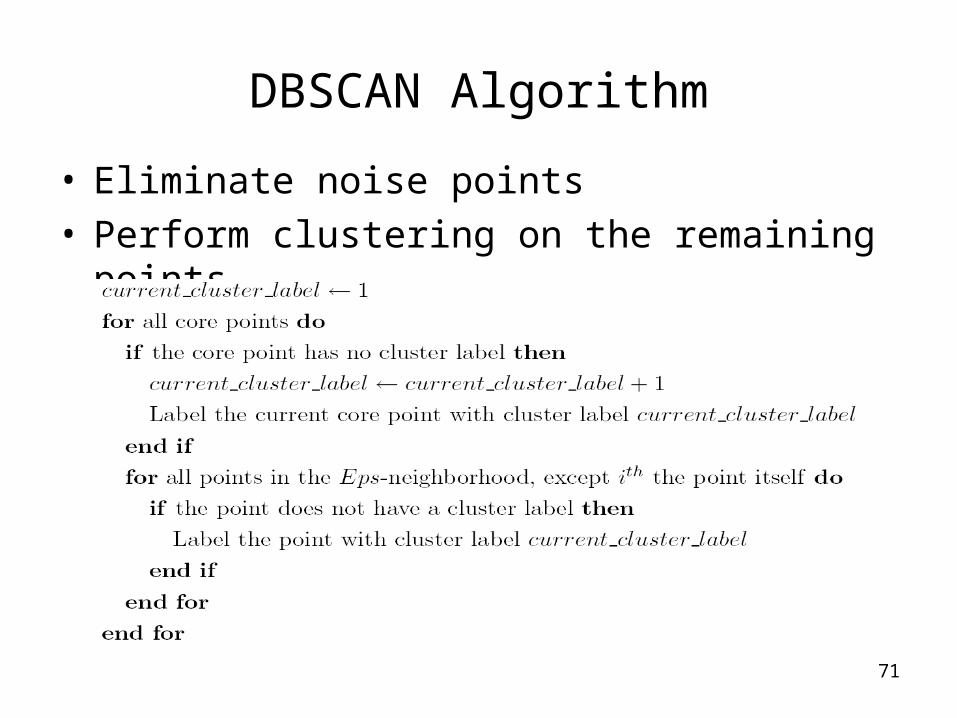
DBSCAN Algorithm
• Eliminate noise points• Perform clustering on the remaining points

72
DBSCAN: Core, Border and Noise Points
Original Points Point types: core, border and noise
Eps = 10, MinPts = 4

73
When DBSCAN Works Well
Original Points Clusters
• Resistant to Noise
• Can handle clusters of different shapes and sizes
74
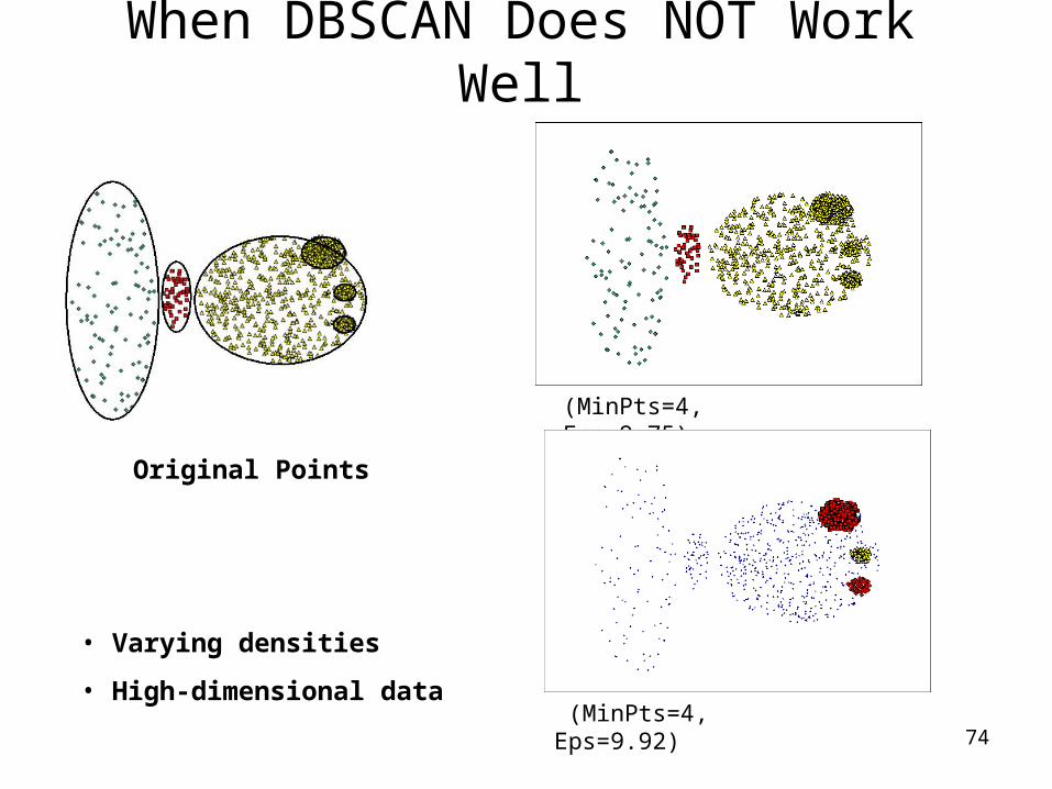
When DBSCAN Does NOT Work Well
Original Points
(MinPts=4, Eps=9.75).
(MinPts=4, Eps=9.92)
• Varying densities
• High-dimensional data

75
DBSCAN: Determining EPS and MinPts• Idea is that for points in a cluster, their kth nearest
neighbors are at roughly the same distance• Noise points have the kth nearest neighbor at farther
distance• So, plot sorted distance of every point to its kth
nearest neighbor

76
Graph-Based Clustering
• Graph-Based clustering uses the proximity graph– Start with the proximity matrix– Consider each point as a node in a graph– Each edge between two nodes has a weight which is
the proximity between the two points– Initially the proximity graph is fully connected – MIN (single-link) and MAX (complete-link) can be
viewed as starting with this graph
• In the simplest case, clusters are connected components in the graph.

77
Graph-Based Clustering: Sparsification
• Clustering may work better– Sparsification techniques keep the connections to the most
similar (nearest) neighbors of a point while breaking the connections to less similar points.
– The nearest neighbors of a point tend to belong to the same class as the point itself.
– This reduces the impact of noise and outliers and sharpens the distinction between clusters.
• Sparsification facilitates the use of graph partitioning algorithms (or algorithms based on graph partitioning algorithms.
– Chameleon and Hypergraph-based Clustering

78
Sparsification in the Clustering Process
79
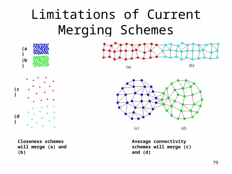
Limitations of Current Merging Schemes
Closeness schemes will merge (a) and (b)
(a)
(b)
(c)
(d)
Average connectivity schemes will merge (c) and (d)

80
Model-Based Clustering Methods
• Attempt to optimize the fit between the data and some mathematical model
• Statistical and AI approach– Conceptual clustering
• A form of clustering in machine learning
• Produces a classification scheme for a set of unlabeled objects
• Finds characteristic description for each concept (class)
– COBWEB (Fisher’87) • A popular a simple method of incremental conceptual learning
• Creates a hierarchical clustering in the form of a classification tree
• Each node refers to a concept and contains a probabilistic description of that concept

81
Cluster Validity
• For supervised classification we have a variety of measures to evaluate how good our model is– Accuracy, precision, recall
• For cluster analysis, the analogous question is how to evaluate the “goodness” of the resulting clusters?
• But “clusters are in the eye of the beholder”!
• Then why do we want to evaluate them?– To avoid finding patterns in noise– To compare clustering algorithms– To compare two sets of clusters– To compare two clusters

82
Clusters found in Random Data
0 0.2 0.4 0.6 0.8 10
0.1
0.2
0.3
0.4
0.5
0.6
0.7
0.8
0.9
1
x
y
Random Points
0 0.2 0.4 0.6 0.8 10
0.1
0.2
0.3
0.4
0.5
0.6
0.7
0.8
0.9
1
x
y
K-means
0 0.2 0.4 0.6 0.8 10
0.1
0.2
0.3
0.4
0.5
0.6
0.7
0.8
0.9
1
x
y
DBSCAN
0 0.2 0.4 0.6 0.8 10
0.1
0.2
0.3
0.4
0.5
0.6
0.7
0.8
0.9
1
x
y
Complete Link

83
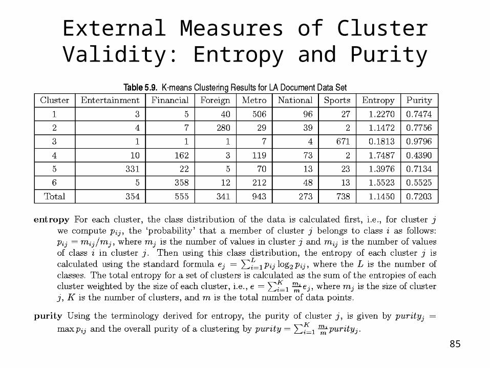
• Numerical measures that are applied to judge various aspects of cluster validity, are classified into the following three types.– External Index: Used to measure the extent to which cluster labels
match externally supplied class labels.• Entropy
– Internal Index: Used to measure the goodness of a clustering structure without respect to external information.
• Sum of Squared Error (SSE)
– Relative Index: Used to compare two different clusterings or clusters.
• Often an external or internal index is used for this function, e.g., SSE or entropy
• Sometimes these are referred to as criteria instead of indices– However, sometimes criterion is the general strategy and index is the
numerical measure that implements the criterion.
Measures of Cluster Validity

84
• Cluster Cohesion: Measures how closely related are objects in a cluster– Example: SSE
• Cluster Separation: Measure how distinct or well-separated a cluster is from other clusters
• Example: Squared Error– Cohesion is measured by the within cluster sum of squares (SSE)
– Separation is measured by the between cluster sum of squares
• Where |Ci| is the size of cluster i
Internal Measures: Cohesion and Separation
i Cx
ii
mxWSS 2)(
i
ii mmCBSS 2)(
85
External Measures of Cluster Validity: Entropy and Purity

86
“The validation of clustering structures is the most difficult and frustrating part of cluster analysis.
Without a strong effort in this direction, cluster analysis will remain a black art accessible only to those true believers who have experience and great courage.”
Algorithms for Clustering Data, Jain and Dubes
Final Comment on Cluster Validity

87
What Is Outlier Discovery?
• What are outliers?– The set of objects are considerably dissimilar from the
remainder of the data– Example: Sports: Michael Jordon, Wayne Gretzky, ...
• Problem– Find top n outlier points
• Applications:– Credit card fraud detection– Telecom fraud detection– Customer segmentation– Medical analysis

88
Outlier Discovery: Statistical Approach
Assume a model underlying distribution that generates data set (e.g. normal distribution)
• Use discordancy tests depending on – data distribution– distribution parameter (e.g., mean, variance)– number of expected outliers
• Drawbacks– most tests are for single attribute– In many cases, data distribution may not be known

89
Outlier Discovery: Distance-Based Approach
• Introduced to counter the main limitations imposed by statistical methods– We need multi-dimensional analysis without knowing data
distribution.
• Distance-based outlier: outlier is an object O in a dataset T such that at least a fraction p of the objects in T lies at a distance greater than D from O
• Algorithms for mining distance-based outliers – Index-based algorithm– Nested-loop algorithm – Cell-based algorithm

90
Outlier Discovery: Deviation-Based Approach
• Identifies outliers by examinining the main characteristics of objects in a group
• Objects that “deviate” from this description are considered outliers
• sequential exception technique – simulates the way in which humans can distinguish unusual
objects from among a series of supposedly like objects
• OLAP data cube technique– uses data cubes to identify regions of anomalies in large
multidimensional data