1

Equity Instruments & Markets: Part IIEquity Instruments & Markets: Part IIB40.3331B40.3331

Relative Valuation and Private Relative Valuation and Private Company ValuationCompany Valuation

Aswath Damodaran

2

The Essence of relative valuation?The Essence of relative valuation?

In relative valuation, the value of an asset is compared to the values assessed by the market for similar or comparable assets.

To do relative valuation then,– we need to identify comparable assets and obtain market values for these

assets

– convert these market values into standardized values, since the absolute prices cannot be compared This process of standardizing creates price multiples.

– compare the standardized value or multiple for the asset being analyzed to the standardized values for comparable asset, controlling for any differences between the firms that might affect the multiple, to judge whether the asset is under or over valued

3

Relative valuation is pervasive…Relative valuation is pervasive…

Most valuations on Wall Street are relative valuations. – Almost 85% of equity research reports are based upon a multiple and

comparables.

– More than 50% of all acquisition valuations are based upon multiples

– Rules of thumb based on multiples are not only common but are often the basis for final valuation judgments.

While there are more discounted cashflow valuations in consulting and corporate finance, they are often relative valuations masquerading as discounted cash flow valuations.– The objective in many discounted cashflow valuations is to back into a

number that has been obtained by using a multiple.

– The terminal value in a significant number of discounted cashflow valuations is estimated using a multiple.

4

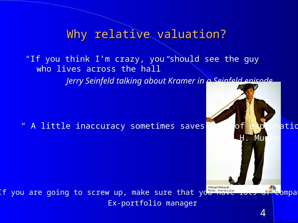
Why relative valuation?Why relative valuation?

“If you think I’m crazy, you should see the guy who lives across the hall”

Jerry Seinfeld talking about Kramer in a Seinfeld episode

“ A little inaccuracy sometimes saves tons of explanation”

H.H. Munro

“ If you are going to screw up, make sure that you have lots of company”

Ex-portfolio manager

5

So, you believe only in intrinsic value? Here’s So, you believe only in intrinsic value? Here’s why you should still care about relative valuewhy you should still care about relative value

Even if you are a true believer in discounted cashflow valuation, presenting your findings on a relative valuation basis will make it more likely that your findings/recommendations will reach a receptive audience.

In some cases, relative valuation can help find weak spots in discounted cash flow valuations and fix them.

The problem with multiples is not in their use but in their abuse. If we can find ways to frame multiples right, we should be able to use them better.

6

Multiples are just standardized estimates of Multiples are just standardized estimates of price…price…

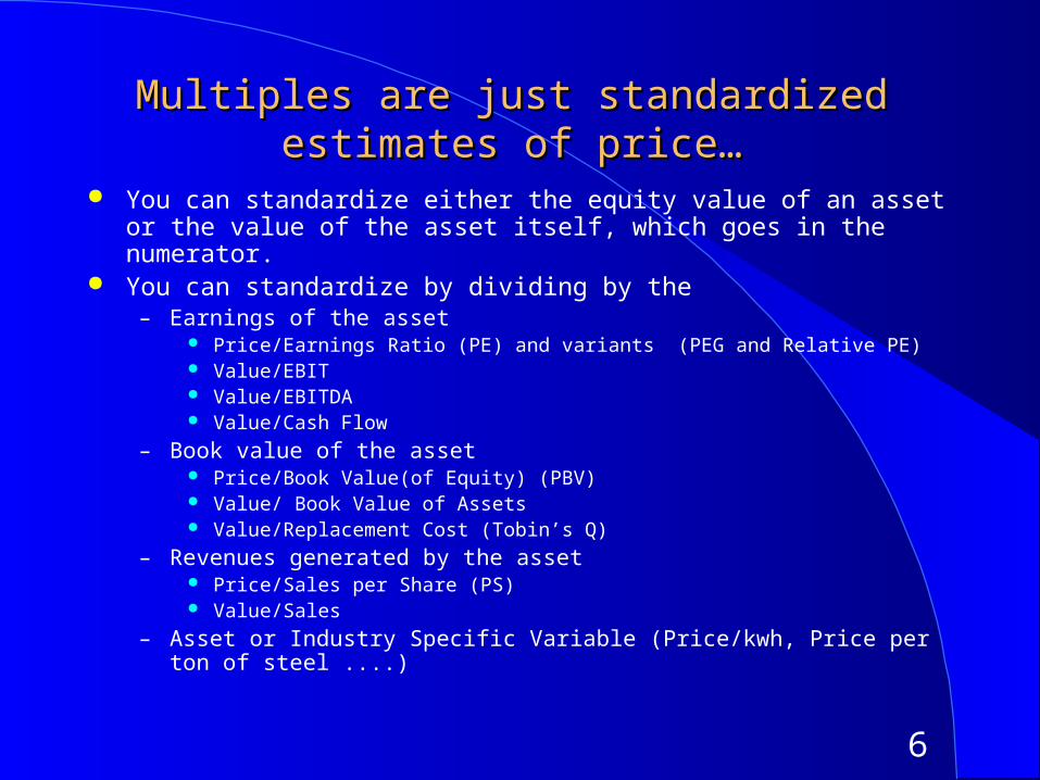
You can standardize either the equity value of an asset or the value of the asset itself, which goes in the numerator.

You can standardize by dividing by the – Earnings of the asset

Price/Earnings Ratio (PE) and variants (PEG and Relative PE) Value/EBIT Value/EBITDA Value/Cash Flow

– Book value of the asset Price/Book Value(of Equity) (PBV) Value/ Book Value of Assets Value/Replacement Cost (Tobin’s Q)

– Revenues generated by the asset Price/Sales per Share (PS) Value/Sales

– Asset or Industry Specific Variable (Price/kwh, Price per ton of steel ....)

7

The Four Steps to Understanding MultiplesThe Four Steps to Understanding Multiples

Define the multiple– In use, the same multiple can be defined in different ways by different users. When

comparing and using multiples, estimated by someone else, it is critical that we understand how the multiples have been estimated

Describe the multiple– Too many people who use a multiple have no idea what its cross sectional

distribution is. If you do not know what the cross sectional distribution of a multiple is, it is difficult to look at a number and pass judgment on whether it is too high or low.

Analyze the multiple– It is critical that we understand the fundamentals that drive each multiple, and the

nature of the relationship between the multiple and each variable. Apply the multiple

– Defining the comparable universe and controlling for differences is far more difficult in practice than it is in theory.

8

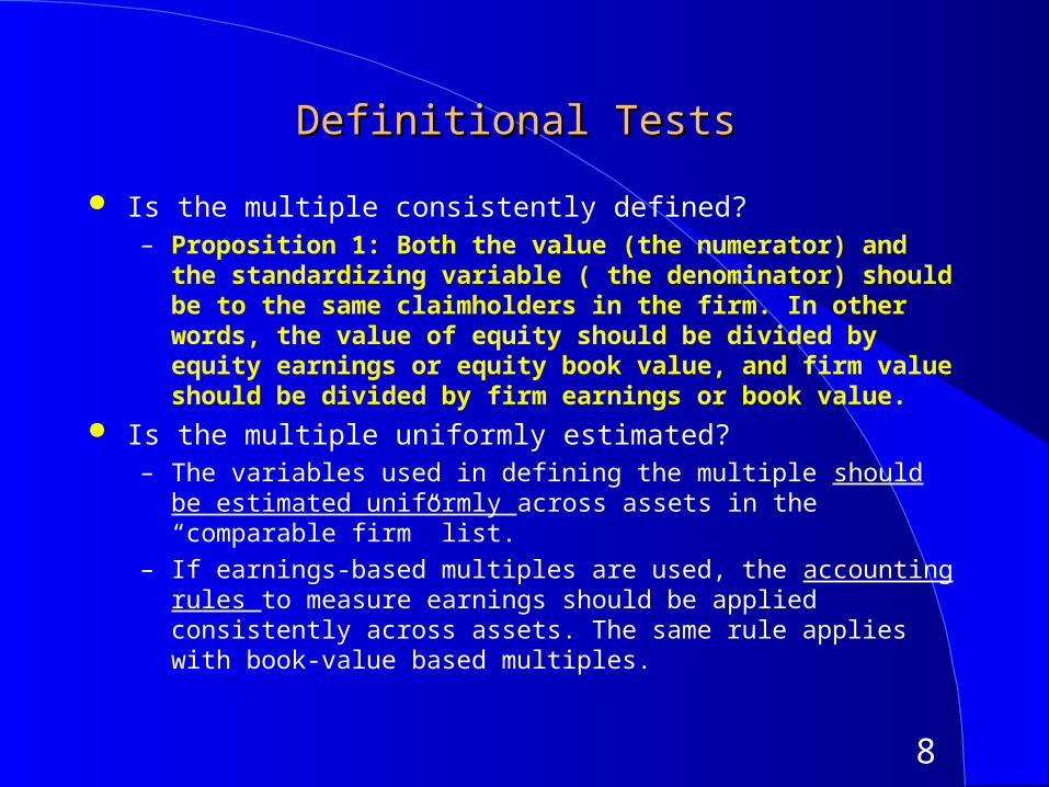
Definitional TestsDefinitional Tests

Is the multiple consistently defined?– Proposition 1: Both the value (the numerator) and the standardizing

variable ( the denominator) should be to the same claimholders in the firm. In other words, the value of equity should be divided by equity earnings or equity book value, and firm value should be divided by firm earnings or book value.

Is the multiple uniformly estimated?– The variables used in defining the multiple should be estimated uniformly

across assets in the “comparable firm” list.

– If earnings-based multiples are used, the accounting rules to measure earnings should be applied consistently across assets. The same rule applies with book-value based multiples.

9

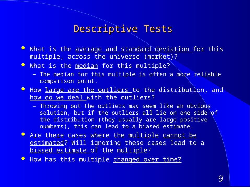
Descriptive TestsDescriptive Tests

What is the average and standard deviation for this multiple, across the universe (market)?

What is the median for this multiple? – The median for this multiple is often a more reliable comparison point.

How large are the outliers to the distribution, and how do we deal with the outliers?– Throwing out the outliers may seem like an obvious solution, but if the

outliers all lie on one side of the distribution (they usually are large positive numbers), this can lead to a biased estimate.

Are there cases where the multiple cannot be estimated? Will ignoring these cases lead to a biased estimate of the multiple?

How has this multiple changed over time?

10

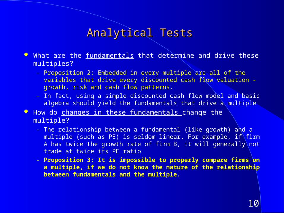
Analytical TestsAnalytical Tests

What are the fundamentals that determine and drive these multiples?– Proposition 2: Embedded in every multiple are all of the variables that

drive every discounted cash flow valuation - growth, risk and cash flow patterns.

– In fact, using a simple discounted cash flow model and basic algebra should yield the fundamentals that drive a multiple

How do changes in these fundamentals change the multiple?– The relationship between a fundamental (like growth) and a multiple

(such as PE) is seldom linear. For example, if firm A has twice the growth rate of firm B, it will generally not trade at twice its PE ratio

– Proposition 3: It is impossible to properly compare firms on a multiple, if we do not know the nature of the relationship between fundamentals and the multiple.

11

Application TestsApplication Tests

Given the firm that we are valuing, what is a “comparable” firm?– While traditional analysis is built on the premise that firms in the same

sector are comparable firms, valuation theory would suggest that a comparable firm is one which is similar to the one being analyzed in terms of fundamentals.

– Proposition 4: There is no reason why a firm cannot be compared with another firm in a very different business, if the two firms have the same risk, growth and cash flow characteristics.

Given the comparable firms, how do we adjust for differences across firms on the fundamentals?– Proposition 5: It is impossible to find an exactly identical firm to the

one you are valuing.

12

Price Earnings Ratio: DefinitionPrice Earnings Ratio: Definition

PE = Market Price per Share / Earnings per Share There are a number of variants on the basic PE ratio in use. They are based

upon how the price and the earnings are defined. Price:

– is usually the current price (though some like to use average price over last 6 months or year)

EPS:– Time variants: EPS in most recent financial year (current), EPS in most recent four

quarters (trailing), EPS expected in next fiscal year or next four quartes (both called forward) or EPS in some future year

– Primary, diluted or partially diluted

– Before or after extraordinary items

– Measured using different accounting rules (options expensed or not, pension fund income counted or not…)

13

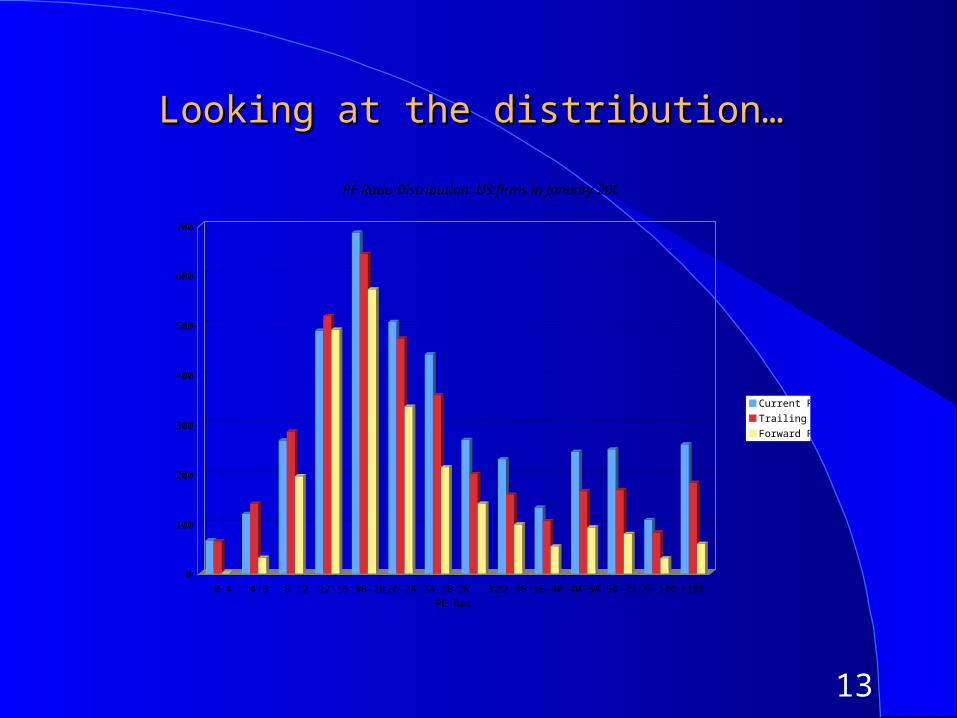
Looking at the distribution…Looking at the distribution…

0

100

200

300

400

500

600

700

0-4 4-8 8-12 12-16 16-20 20-24 24-28 28 - 32 32-36 36-40 40-50 50-75 75-100 >100

PE Ratio

PE Ratio Distribution: US firms in January 2005

Current PE

Trailing PE

Forward PE

14

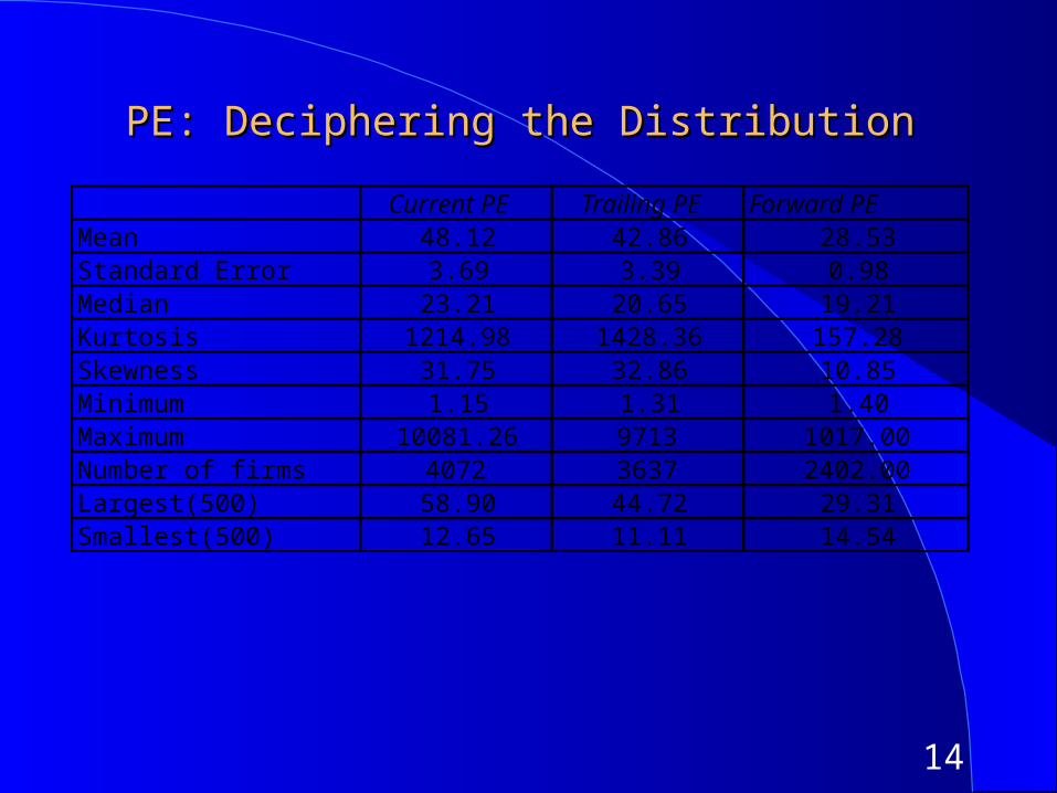
PE: Deciphering the DistributionPE: Deciphering the Distribution

Current PE Trailing PE Forward PEMean 48.12 42.86 28.53Standard Error 3.69 3.39 0.98Median 23.21 20.65 19.21Kurtosis 1214.98 1428.36 157.28Skewness 31.75 32.86 10.85Minimum 1.15 1.31 1.40Maximum 10081.26 9713 1017.00Number of firms 4072 3637 2402.00Largest(500) 58.90 44.72 29.31Smallest(500) 12.65 11.11 14.54

15

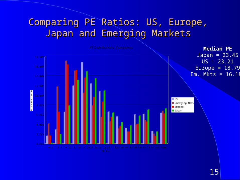
Comparing PE Ratios: US, Europe, Japan and Comparing PE Ratios: US, Europe, Japan and Emerging MarketsEmerging Markets

Median PEJapan = 23.45

US = 23.21Europe = 18.79

Em. Mkts = 16.18

0.00%

2.00%

4.00%

6.00%

8.00%

10.00%

12.00%

14.00%

16.00%

18.00%

% of firms in market

0-4 4-8 8-12 12-16 16-20 20-24 24-28 28 - 32 32-36 36-40 40-50 50-75 75-100 >100

PE Ratio

PE Distributions: Comparison

US

Emerging Markets

Europe

Japan

16

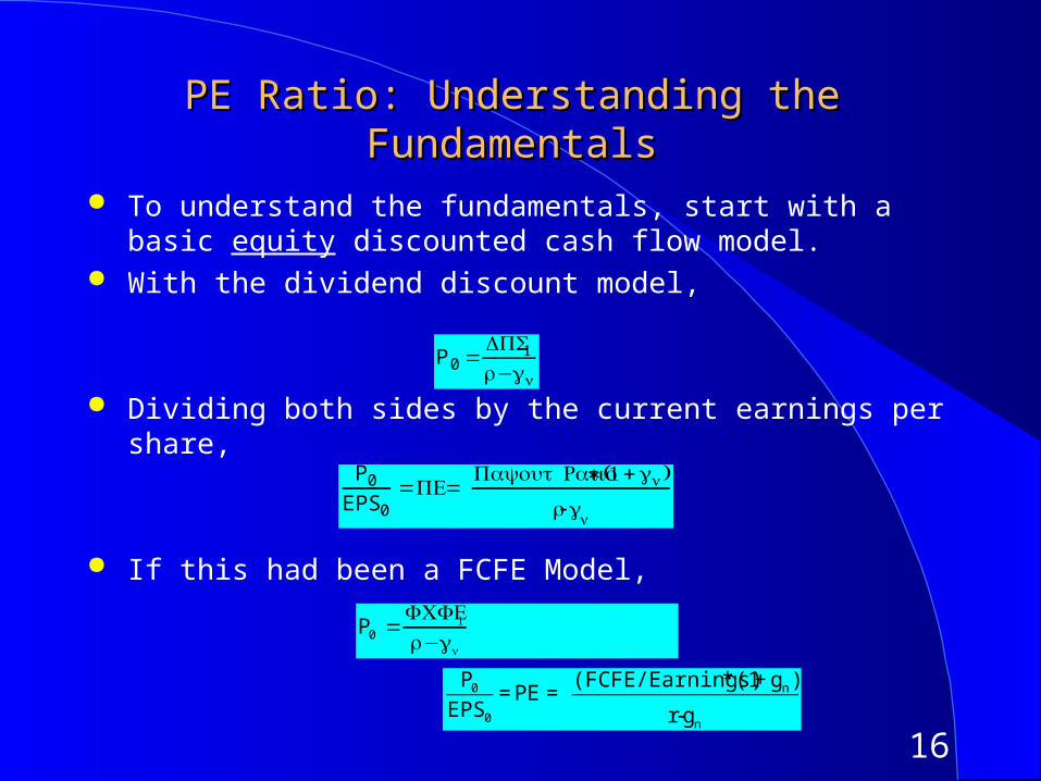
PE Ratio: Understanding the FundamentalsPE Ratio: Understanding the Fundamentals

To understand the fundamentals, start with a basic equity discounted cash flow model.

With the dividend discount model,

Dividing both sides by the current earnings per share,

If this had been a FCFE Model,

P 0 =DPS1r−gn

P0

EPS0=PE=

Payout Ratio* (1 +gn)

r-gn

P0 =FCFE1

r−gn

€

P0

EPS0

= PE = (FCFE/Earnings)* (1+ gn )

r-gn

17

PE Ratio and FundamentalsPE Ratio and Fundamentals

Proposition: Other things held equal, higher growth firms will have higher PE ratios than lower growth firms.

Proposition: Other things held equal, higher risk firms will have lower PE ratios than lower risk firms

Proposition: Other things held equal, firms with lower reinvestment needs will have higher PE ratios than firms with higher reinvestment rates.

Of course, other things are difficult to hold equal since high growth firms, tend to have risk and high reinvestment rats.

18

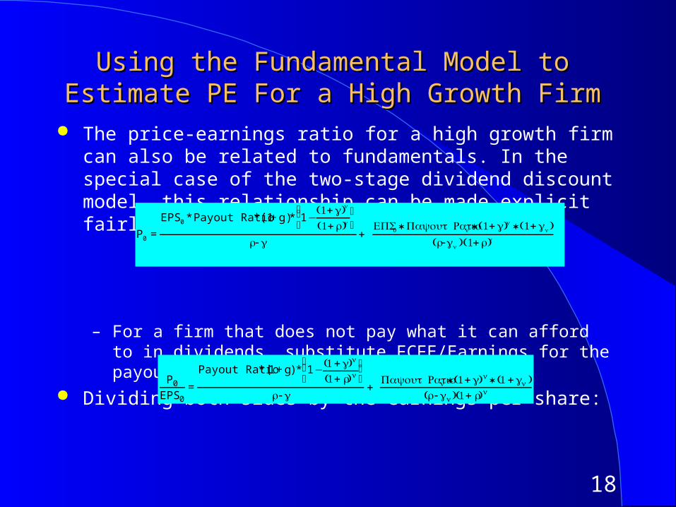
Using the Fundamental Model to Estimate PE Using the Fundamental Model to Estimate PE For a High Growth FirmFor a High Growth Firm

The price-earnings ratio for a high growth firm can also be related to fundamentals. In the special case of the two-stage dividend discount model, this relationship can be made explicit fairly simply:

– For a firm that does not pay what it can afford to in dividends, substitute FCFE/Earnings for the payout ratio.

Dividing both sides by the earnings per share:

P0 =

EPS0 * Payout Ratio *(1+ g)* 1−(1+ )g n

(1+ )r n

⎛ ⎝ ⎜ ⎞

⎠

r-g+

EPS0 * Payout Ration * (1+ )g n * (1+gn)(r-gn )(1+ )r n

P0

EPS0=

Payout Ratio * (1 + g) * 1−(1+g)n

(1+ r)n ⎛

⎝ ⎜ ⎞

⎠ ⎟

r -g+

Payout Ration * (1+g)n* (1 +gn )(r -gn)(1+ r)n

19

Expanding the ModelExpanding the Model

In this model, the PE ratio for a high growth firm is a function of growth, risk and payout, exactly the same variables that it was a function of for the stable growth firm.

The only difference is that these inputs have to be estimated for two phases - the high growth phase and the stable growth phase.

Expanding to more than two phases, say the three stage model, will mean that risk, growth and cash flow patterns in each stage.

20

A Simple ExampleA Simple Example

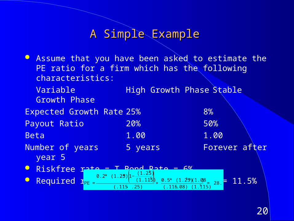
Assume that you have been asked to estimate the PE ratio for a firm which has the following characteristics:

Variable High Growth Phase Stable Growth Phase

Expected Growth Rate 25% 8%

Payout Ratio 20% 50%

Beta 1.00 1.00

Number of years 5 years Forever after year 5 Riskfree rate = T.Bond Rate = 6% Required rate of return = 6% + 1(5.5%)= 11.5%

€

PE =

0.2 * (1.25) * 1−(1.25)5

(1.115)5

⎛

⎝ ⎜

⎞

⎠ ⎟

(.115 - .25)+

0.5 * (1.25)5 * (1.08)

(.115 - .08) (1.115)5 = 28.75

21

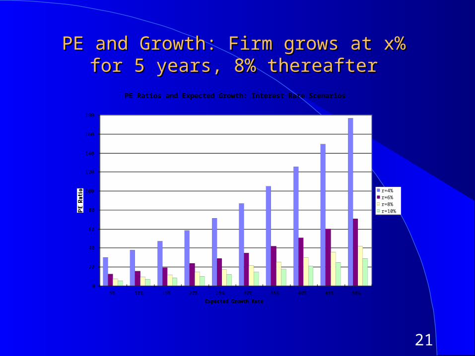
PE and Growth: Firm grows at x% for 5 years, PE and Growth: Firm grows at x% for 5 years, 8% thereafter8% thereafter

PE Ratios and Expected Growth: Interest Rate Scenarios

0

20

40

60

80

100

120

140

160

180

5% 10% 15% 20% 25% 30% 35% 40% 45% 50%

Expected Growth Rate

PE Ratio

r=4%r=6%r=8%r=10%

22

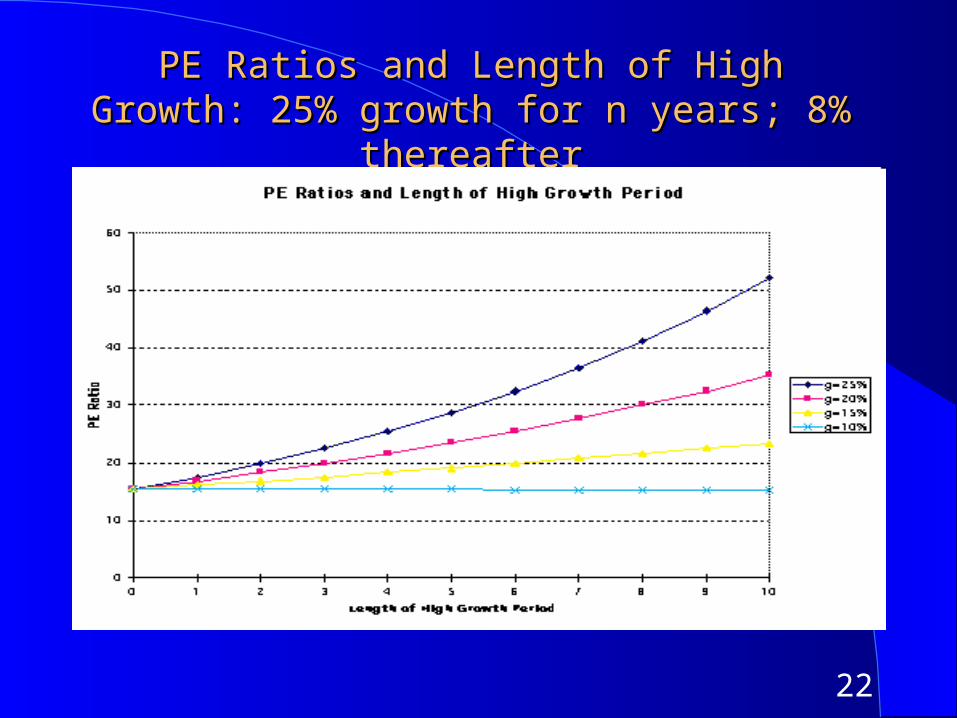
PE Ratios and Length of High Growth: 25% PE Ratios and Length of High Growth: 25% growth for n years; 8% thereaftergrowth for n years; 8% thereafter

23

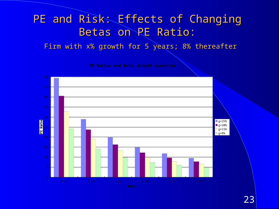
PE and Risk: Effects of Changing Betas on PE PE and Risk: Effects of Changing Betas on PE Ratio:Ratio:

Firm with x% growth for 5 years; 8% thereafterFirm with x% growth for 5 years; 8% thereafter

PE Ratios and Beta: Growth Scenarios

0

5

10

15

20

25

30

35

40

45

50

0.75 1.00 1.25 1.50 1.75 2.00

Beta

PE Ratio

g=25%g=20%g=15%g=8%

24

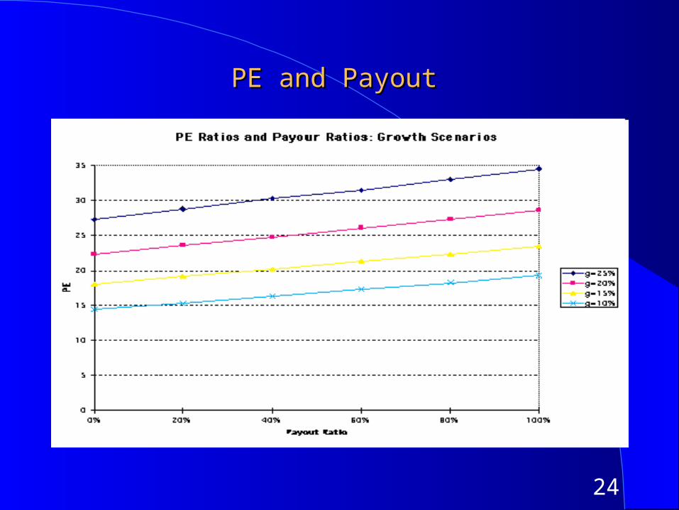
PE and PayoutPE and Payout

25

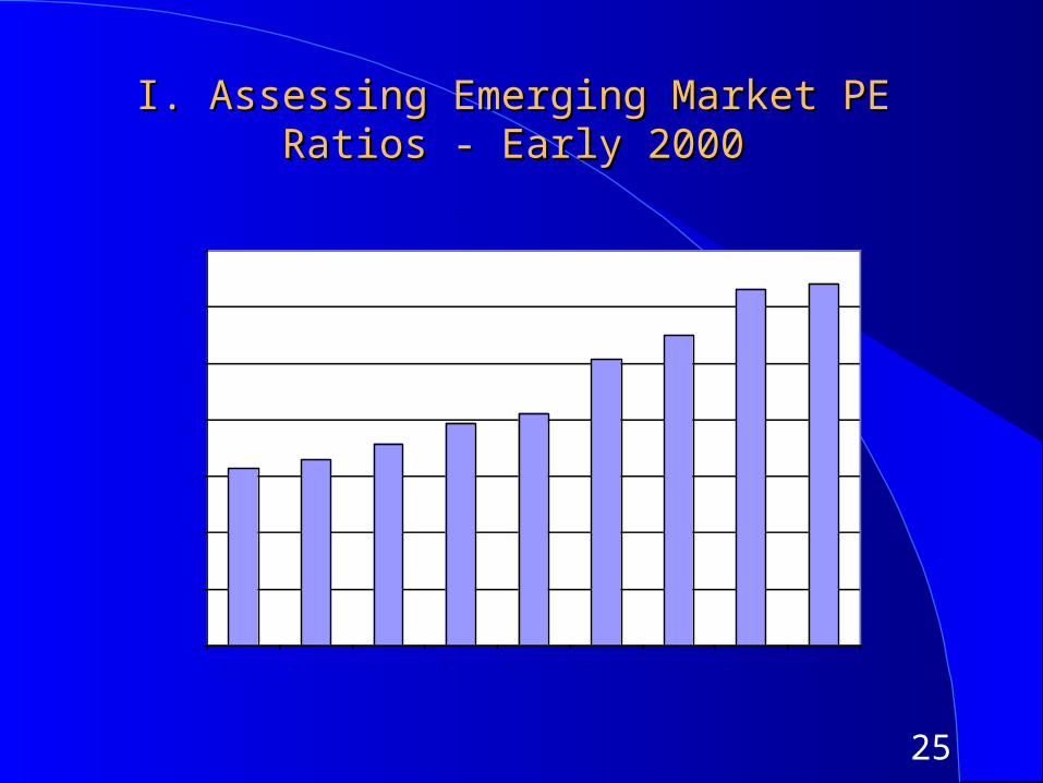
I. Assessing Emerging Market PE Ratios - I. Assessing Emerging Market PE Ratios - Early 2000Early 2000

PE: Emerging Markets

0

5

10

15

20

25

30

35

Mexico Malaysia Singapore Taiwan Hong Kong Venezuela Brazil Argentina Chile

26

Comparisons across countriesComparisons across countries

In July 2000, a market strategist is making the argument that Brazil and Venezuela are cheap relative to Chile, because they have much lower PE ratios. Would you agree?

Yes No What are some of the factors that may cause one market’s PE ratios to

be lower than another market’s PE?

27

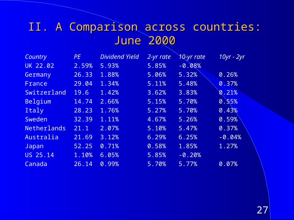
II. A Comparison across countries: June 2000II. A Comparison across countries: June 2000

Country PE Dividend Yield 2-yr rate 10-yr rate 10yr - 2yrUK 22.02 2.59% 5.93% 5.85% -0.08%Germany 26.33 1.88% 5.06% 5.32% 0.26%France 29.04 1.34% 5.11% 5.48% 0.37%Switzerland 19.6 1.42% 3.62% 3.83% 0.21%Belgium 14.74 2.66% 5.15% 5.70% 0.55%Italy 28.23 1.76% 5.27% 5.70% 0.43%Sweden 32.39 1.11% 4.67% 5.26% 0.59%Netherlands 21.1 2.07% 5.10% 5.47% 0.37%Australia 21.69 3.12% 6.29% 6.25% -0.04%Japan 52.25 0.71% 0.58% 1.85% 1.27%US 25.14 1.10% 6.05% 5.85% -0.20%Canada 26.14 0.99% 5.70% 5.77% 0.07%

28

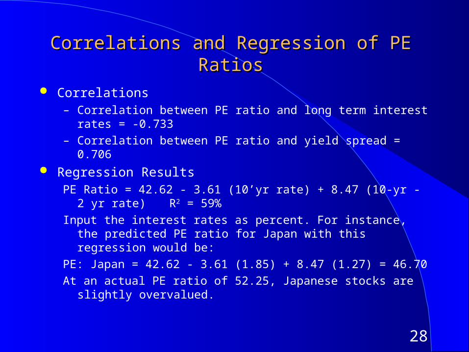
Correlations and Regression of PE RatiosCorrelations and Regression of PE Ratios

Correlations– Correlation between PE ratio and long term interest rates = -0.733

– Correlation between PE ratio and yield spread = 0.706 Regression Results

PE Ratio = 42.62 - 3.61 (10’yr rate) + 8.47 (10-yr - 2 yr rate) R2 = 59%

Input the interest rates as percent. For instance, the predicted PE ratio for Japan with this regression would be:

PE: Japan = 42.62 - 3.61 (1.85) + 8.47 (1.27) = 46.70

At an actual PE ratio of 52.25, Japanese stocks are slightly overvalued.

29

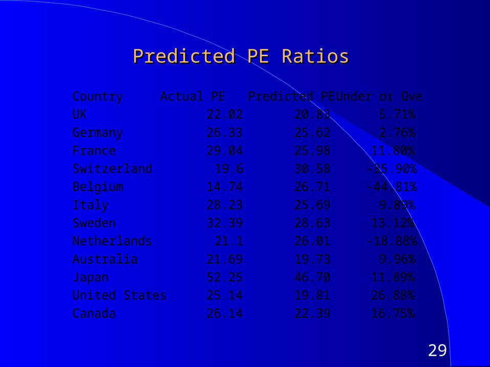
Predicted PE RatiosPredicted PE Ratios

Country Actual PE Predicted PE Under or Over ValuedUK 22.02 20.83 5.71%Germany 26.33 25.62 2.76%France 29.04 25.98 11.80%Switzerland 19.6 30.58 -35.90%Belgium 14.74 26.71 -44.81%Italy 28.23 25.69 9.89%Sweden 32.39 28.63 13.12%Netherlands 21.1 26.01 -18.88%Australia 21.69 19.73 9.96%Japan 52.25 46.70 11.89%United States 25.14 19.81 26.88%Canada 26.14 22.39 16.75%

30

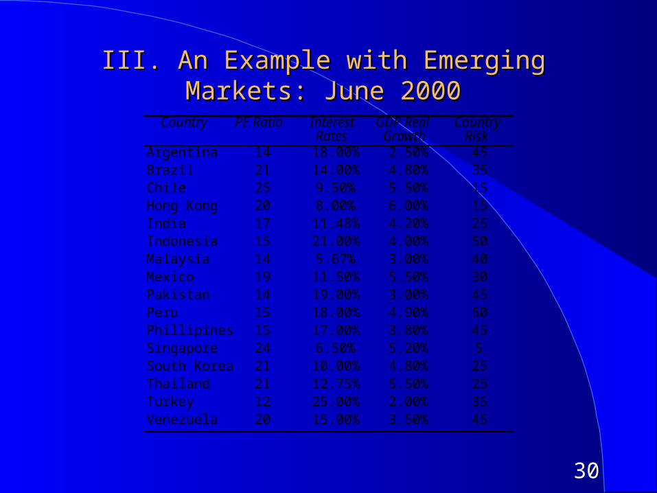
III. An Example with Emerging Markets: June III. An Example with Emerging Markets: June 20002000

Country PE Ratio Interest Rates

GDP Real Growth

Country Risk

Argentina 14 18.00% 2.50% 45Brazil 21 14.00% 4.80% 35Chile 25 9.50% 5.50% 15Hong Kong 20 8.00% 6.00% 15India 17 11.48% 4.20% 25Indonesia 15 21.00% 4.00% 50Malaysia 14 5.67% 3.00% 40Mexico 19 11.50% 5.50% 30Pakistan 14 19.00% 3.00% 45Peru 15 18.00% 4.90% 50Phillipines 15 17.00% 3.80% 45Singapore 24 6.50% 5.20% 5South Korea 21 10.00% 4.80% 25Thailand 21 12.75% 5.50% 25Turkey 12 25.00% 2.00% 35Venezuela 20 15.00% 3.50% 45

31

Regression ResultsRegression Results

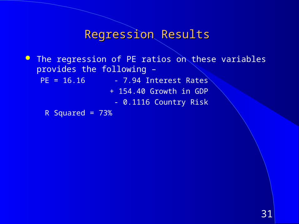
The regression of PE ratios on these variables provides the following –PE = 16.16 - 7.94 Interest Rates

+ 154.40 Growth in GDP

- 0.1116 Country Risk

R Squared = 73%

32

Predicted PE RatiosPredicted PE Ratios

Country PE Ratio Interest Rates

GDP Real Growth

Country Risk

Predicted PE

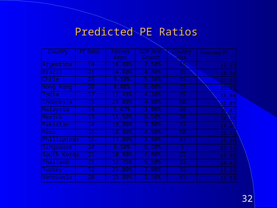
Argentina 14 18.00% 2.50% 45 13.57Brazil 21 14.00% 4.80% 35 18.55Chile 25 9.50% 5.50% 15 22.22Hong Kong 20 8.00% 6.00% 15 23.11India 17 11.48% 4.20% 25 18.94Indonesia 15 21.00% 4.00% 50 15.09Malaysia 14 5.67% 3.00% 40 15.87Mexico 19 11.50% 5.50% 30 20.39Pakistan 14 19.00% 3.00% 45 14.26Peru 15 18.00% 4.90% 50 16.71Phillipines 15 17.00% 3.80% 45 15.65Singapore 24 6.50% 5.20% 5 23.11South Korea 21 10.00% 4.80% 25 19.98Thailand 21 12.75% 5.50% 25 20.85Turkey 12 25.00% 2.00% 35 13.35Venezuela 20 15.00% 3.50% 45 15.35

33

IV. Comparisons of PE across time: PE Ratio IV. Comparisons of PE across time: PE Ratio for the S&P 500for the S&P 500

PE Ratio for S&P 500: 1960-2004

0

5

10

15

20

25

30

35

1960 1962 1964 1966 1968 1970 1972 1974 1976 1978 1980 1982 1984 1986 1988 1990 1992 1994 1996 1998 2000 2002 2004

PE Ratio

Average over period = 16.82

34

Is low (high) PE cheap (expensive)?Is low (high) PE cheap (expensive)?

A market strategist argues that stocks are over priced because the PE ratio today is too high relative to the average PE ratio across time. Do you agree? Yes No

If you do not agree, what factors might explain the higher PE ratio today?

35

E/P Ratios , T.Bond Rates and Term StructureE/P Ratios , T.Bond Rates and Term Structure

EP Ratios and Interest Rates: S&P 500

-2.00%

0.00%

2.00%

4.00%

6.00%

8.00%

10.00%

12.00%

14.00%

16.00%

1960 1962 1964 1966 1968 1970 1972 1974 1976 1978 1980 1982 1984 1986 1988 1990 1992 1994 1996 1998 2000 2002 2004

Year

Earnings Yield

T.Bond Rate

Bond-Bill

36

Regression ResultsRegression Results

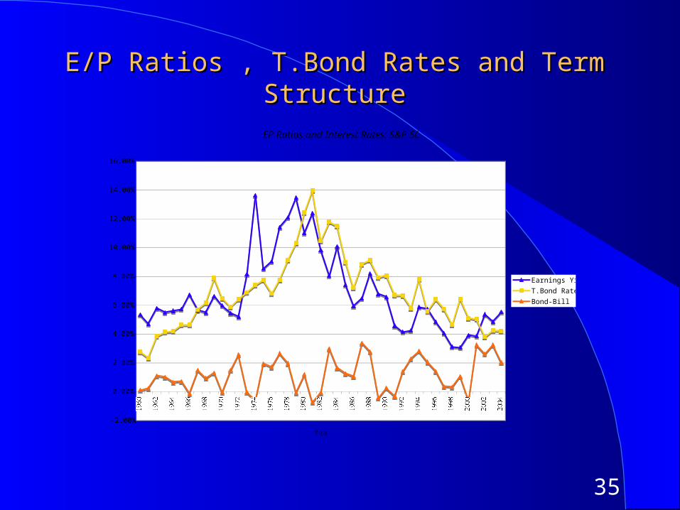
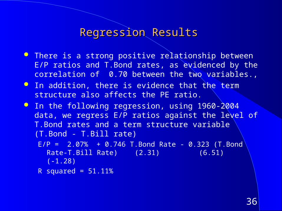
There is a strong positive relationship between E/P ratios and T.Bond rates, as evidenced by the correlation of 0.70 between the two variables.,

In addition, there is evidence that the term structure also affects the PE ratio.

In the following regression, using 1960-2004 data, we regress E/P ratios against the level of T.Bond rates and a term structure variable (T.Bond - T.Bill rate)E/P = 2.07% + 0.746 T.Bond Rate - 0.323 (T.Bond Rate-T.Bill Rate)

(2.31) (6.51) (-1.28)

R squared = 51.11%

37

Estimate the E/P Ratio TodayEstimate the E/P Ratio Today

T. Bond Rate = T.Bond Rate - T.Bill Rate = Expected E/P Ratio = Expected PE Ratio =

38

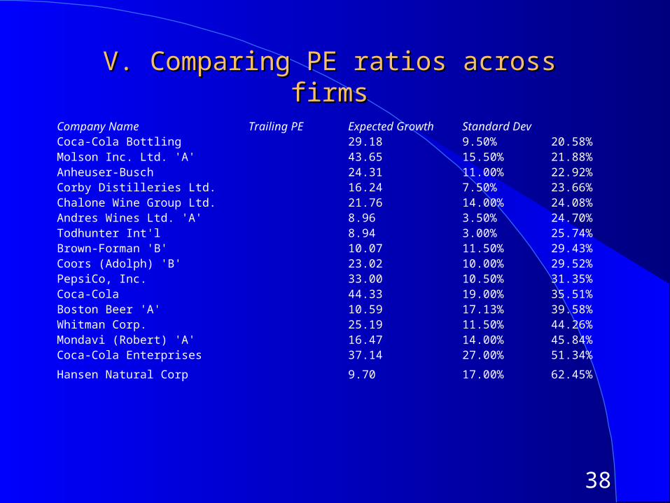
V. Comparing PE ratios across firmsV. Comparing PE ratios across firms

Company Name Trailing PE Expected Growth Standard DevCoca-Cola Bottling 29.18 9.50% 20.58%Molson Inc. Ltd. 'A' 43.65 15.50% 21.88%Anheuser-Busch 24.31 11.00% 22.92%Corby Distilleries Ltd. 16.24 7.50% 23.66%Chalone Wine Group Ltd. 21.76 14.00% 24.08%Andres Wines Ltd. 'A' 8.96 3.50% 24.70%Todhunter Int'l 8.94 3.00% 25.74%Brown-Forman 'B' 10.07 11.50% 29.43%Coors (Adolph) 'B' 23.02 10.00% 29.52%PepsiCo, Inc. 33.00 10.50% 31.35%Coca-Cola 44.33 19.00% 35.51%Boston Beer 'A' 10.59 17.13% 39.58%Whitman Corp. 25.19 11.50% 44.26%Mondavi (Robert) 'A' 16.47 14.00% 45.84%Coca-Cola Enterprises 37.14 27.00% 51.34%

Hansen Natural Corp 9.70 17.00% 62.45%

39

A QuestionA Question

You are reading an equity research report on this sector, and the analyst claims that Andres Wine and Hansen Natural are under valued because they have low PE ratios. Would you agree?

Yes No Why or why not?

40

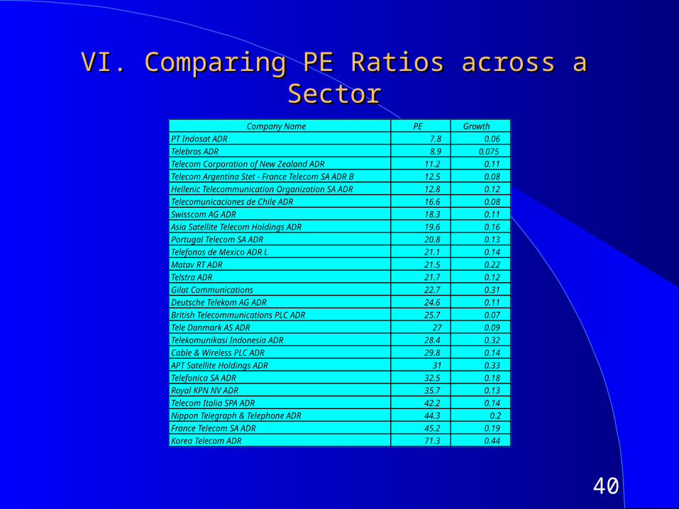
VI. Comparing PE Ratios across a SectorVI. Comparing PE Ratios across a Sector

Company Name PE GrowthPT Indosat ADR 7.8 0.06Telebras ADR 8.9 0.075Telecom Corporation of New Zealand ADR 11.2 0.11Telecom Argentina Stet - France Telecom SA ADR B 12.5 0.08Hellenic Telecommunication Organization SA ADR 12.8 0.12Telecomunicaciones de Chile ADR 16.6 0.08Swisscom AG ADR 18.3 0.11Asia Satellite Telecom Holdings ADR 19.6 0.16Portugal Telecom SA ADR 20.8 0.13Telefonos de Mexico ADR L 21.1 0.14Matav RT ADR 21.5 0.22Telstra ADR 21.7 0.12Gilat Communications 22.7 0.31Deutsche Telekom AG ADR 24.6 0.11British Telecommunications PLC ADR 25.7 0.07Tele Danmark AS ADR 27 0.09Telekomunikasi Indonesia ADR 28.4 0.32Cable & Wireless PLC ADR 29.8 0.14APT Satellite Holdings ADR 31 0.33Telefonica SA ADR 32.5 0.18Royal KPN NV ADR 35.7 0.13Telecom Italia SPA ADR 42.2 0.14Nippon Telegraph & Telephone ADR 44.3 0.2France Telecom SA ADR 45.2 0.19Korea Telecom ADR 71.3 0.44

41

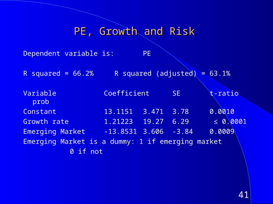
PE, Growth and RiskPE, Growth and Risk

Dependent variable is: PE

R squared = 66.2% R squared (adjusted) = 63.1%

Variable Coefficient SE t-ratio prob

Constant 13.1151 3.471 3.78 0.0010

Growth rate 1.21223 19.27 6.29 ≤ 0.0001

Emerging Market -13.8531 3.606 -3.84 0.0009

Emerging Market is a dummy: 1 if emerging market

0 if not

42

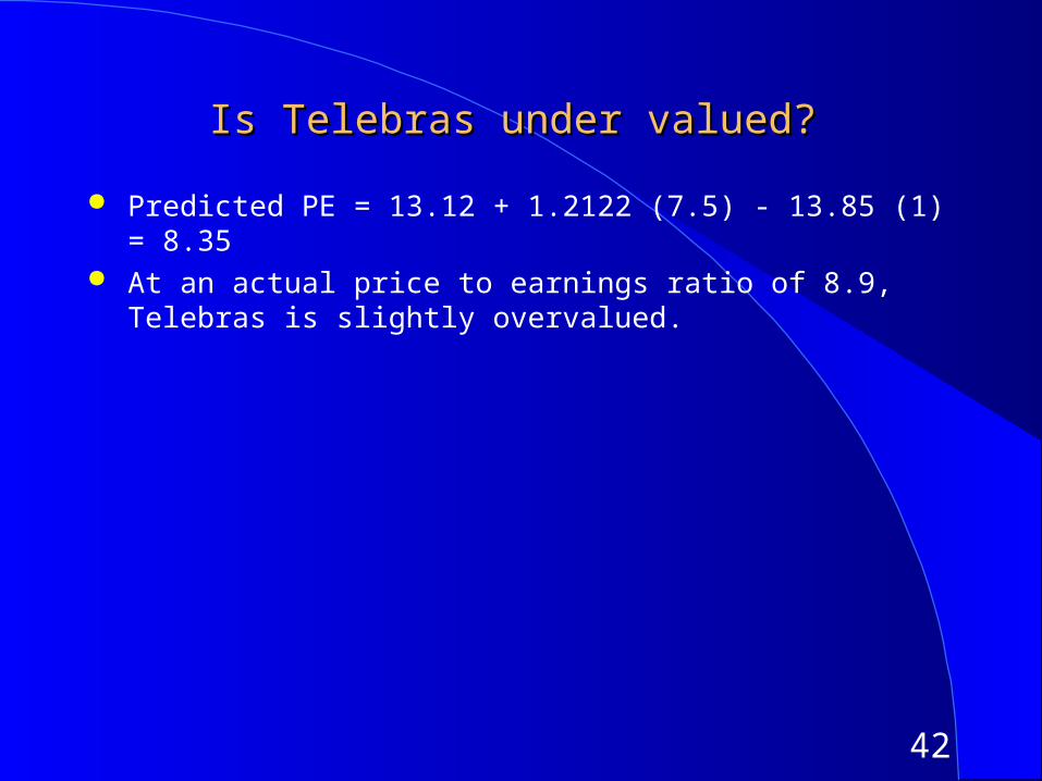
Is Telebras under valued?Is Telebras under valued?

Predicted PE = 13.12 + 1.2122 (7.5) - 13.85 (1) = 8.35 At an actual price to earnings ratio of 8.9, Telebras is slightly

overvalued.

43

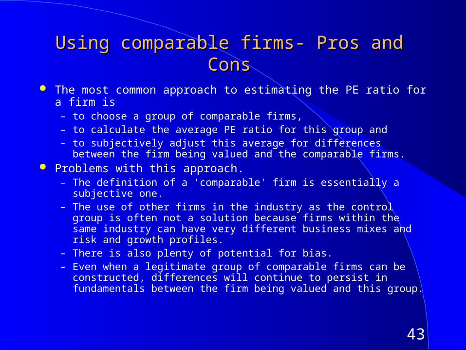
Using comparable firms- Pros and ConsUsing comparable firms- Pros and Cons

The most common approach to estimating the PE ratio for a firm is – to choose a group of comparable firms,– to calculate the average PE ratio for this group and– to subjectively adjust this average for differences between the firm being

valued and the comparable firms. Problems with this approach.

– The definition of a 'comparable' firm is essentially a subjective one. – The use of other firms in the industry as the control group is often not a

solution because firms within the same industry can have very different business mixes and risk and growth profiles.

– There is also plenty of potential for bias. – Even when a legitimate group of comparable firms can be constructed,

differences will continue to persist in fundamentals between the firm being valued and this group.

44

Using the entire crosssection: A regression Using the entire crosssection: A regression approachapproach

In contrast to the 'comparable firm' approach, the information in the entire cross-section of firms can be used to predict PE ratios.

The simplest way of summarizing this information is with a multiple regression, with the PE ratio as the dependent variable, and proxies for risk, growth and payout forming the independent variables.

45

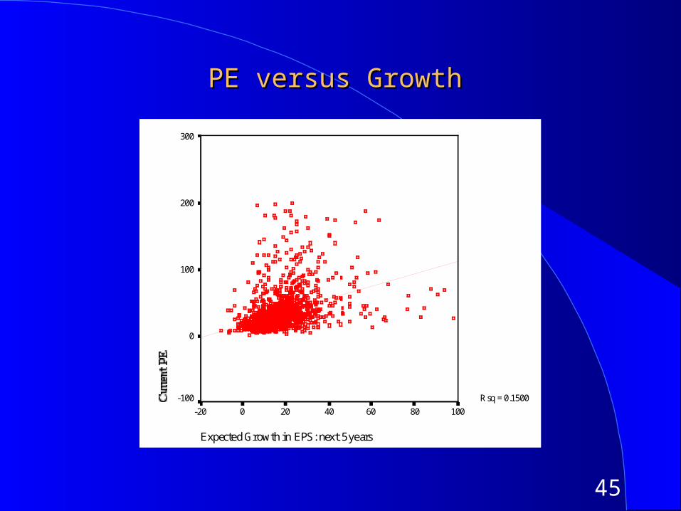
PE versus GrowthPE versus Growth

Expected Growth in EPS: next 5 years

100806040200-20

Current PE

300

200

100

0

-100 Rsq = 0.1500

46

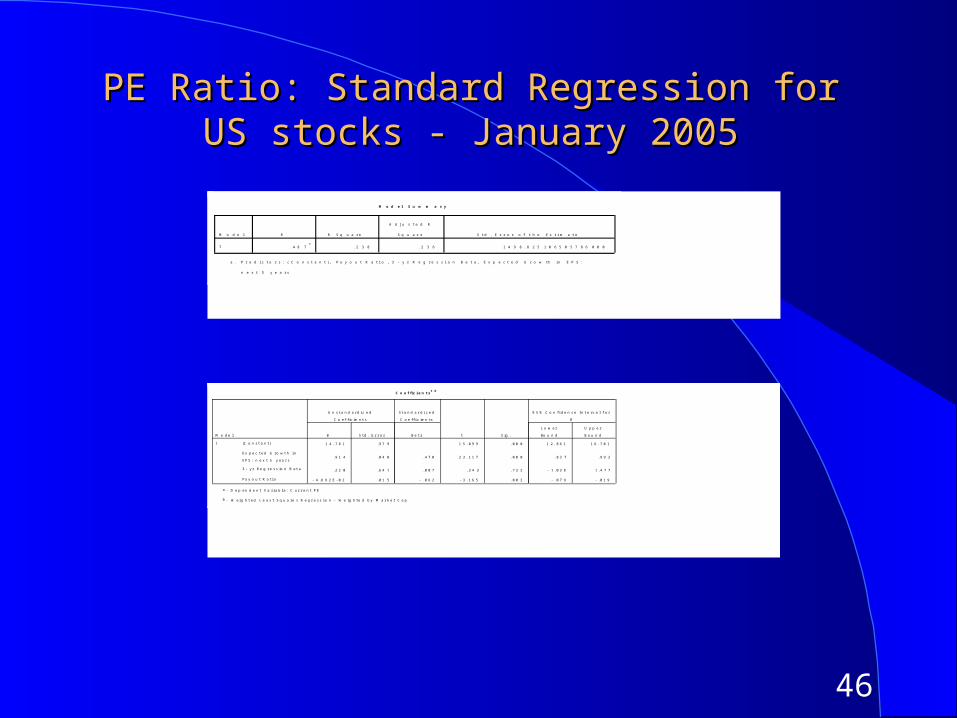
PE Ratio: Standard Regression for US stocks - PE Ratio: Standard Regression for US stocks - January 2005January 2005

M o d e l S u m m a r y

. 4 8 7a

. 2 3 8 . 2 3 6 1 4 9 8 . 8 2 5 1 0 6 5 0 5 7 8 6 0 0 0

M o d e l

1

R R S q u a r e

A d j u s t e d R

S q u a r e S t d . E r r o r o f t h e E s t i m a t e

P r e d i c t o r s : ( C o n s t a n t ) , P a y o u t R a t i o , 3 - y r R e g r e s s i o n B e t a , E x p e c t e d G r o w th i n E P S :

n e x t 5 y e a r s

a .

C o e f fic i e n t sa ,b

1 4 . 7 8 1 . 9 7 9 1 5 . 0 9 9 . 0 0 0 1 2 . 8 6 1 1 6 . 7 0 1

. 9 1 4 . 0 4 0 . 4 7 0 2 3 . 1 1 7 . 0 0 0 . 8 3 7 . 9 9 2

. 2 2 0 . 6 4 1 . 0 0 7 . 3 4 3 . 7 3 2 - 1 . 0 3 8 1 . 4 7 7

- 4 .8 9 2 E - 0 2 . 0 1 5 - . 0 6 2 - 3 . 1 6 5 . 0 0 2 - . 0 7 9 - . 0 1 9

(C o n s t a n t )

Ex p e c t ed G ro w t h i n

EP S : n e x t 5 y ea r s

3 - y r R e g r e s s io n B e t a

P a y o u t R a t i o

M o d e l

1

B S t d . E r r o r

U n s t a n d a r d iz e d

C o e f f ic ie n t s

B e t a

St a n d a r d i z e d

C o e f f i c ie n ts

t S ig .

L o w er

Bo u n d

U p p e r

B o u n d

9 5 % C o n f i d e n c e I n t e rv a l f o r

B

D e p en d e n t V a r i a b l e : C u r r e n t P Ea .

W e i g h t ed L e a s t S q u a re s R e g r e s s i o n - W e ig h te d b y M a r k e t C a pb .

47

Problems with the regression methodologyProblems with the regression methodology

The basic regression assumes a linear relationship between PE ratios and the financial proxies, and that might not be appropriate.

The basic relationship between PE ratios and financial variables itself might not be stable, and if it shifts from year to year, the predictions from the model may not be reliable.

The independent variables are correlated with each other. For example, high growth firms tend to have high risk. This multi-collinearity makes the coefficients of the regressions unreliable and may explain the large changes in these coefficients from period to period.

48

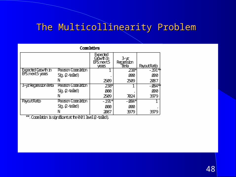
The Multicollinearity ProblemThe Multicollinearity Problem

Correlations

1 .238** -.191**. .000 .000

2509 2509 2087.238** 1 -.084**.000 . .0002509 7024 3979-.191** -.084** 1.000 .000 .2087 3979 3979

Pearson CorrelationSig. (2-tailed)NPearson CorrelationSig. (2-tailed)NPearson CorrelationSig. (2-tailed)N

Expected Growth inEPS: next 5 years

3-yr Regression Beta

Payout Ratio

ExpectedGrowth inEPS: next 5

years

3-yrRegression

Beta Payout Ratio

Correlation is significant at the 0.01 level (2-tailed).**.

49

Using the PE ratio regressionUsing the PE ratio regression

Assume that you were given the following information for Dell. The firm has an expected growth rate of 10%, a beta of 1.20 and pays no dividends. Based upon the regression, estimate the predicted PE ratio for Dell. Predicted PE =

Dell is actually trading at 22 times earnings. What does the predicted PE tell you?

50

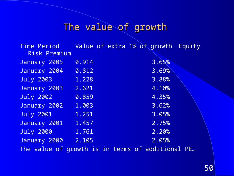
The value of growthThe value of growth

Time Period Value of extra 1% of growth Equity Risk Premium

January 2005 0.914 3.65%

January 2004 0.812 3.69%

July 2003 1.228 3.88%

January 2003 2.621 4.10%

July 2002 0.859 4.35%

January 2002 1.003 3.62%

July 2001 1.251 3.05%

January 2001 1.457 2.75%

July 2000 1.761 2.20%

January 2000 2.105 2.05%

The value of growth is in terms of additional PE…

51

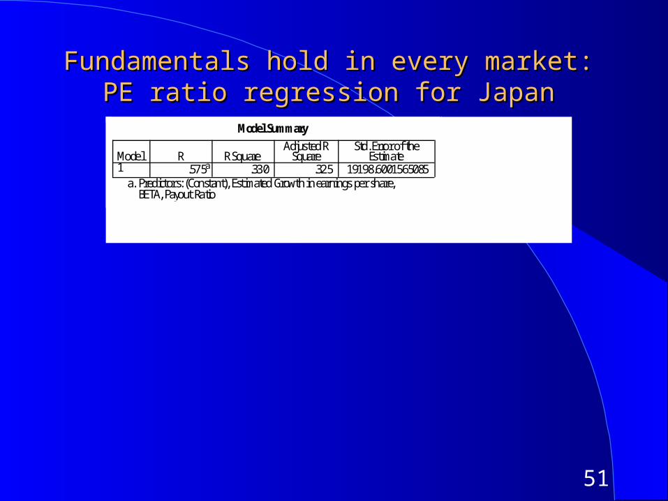
Fundamentals hold in every market: PE ratio Fundamentals hold in every market: PE ratio regression for Japanregression for Japan

Model Summary

.575a .330 .325 19198.6001565085Model1

R R SquareAdjusted R

SquareStd. Error of the

Estimate

Predictors: (Constant), Estimated Growth in earnings per share,BETA, Payout Ratio

a.

52

Investment Strategies that compare PE to the Investment Strategies that compare PE to the expected growth rateexpected growth rate

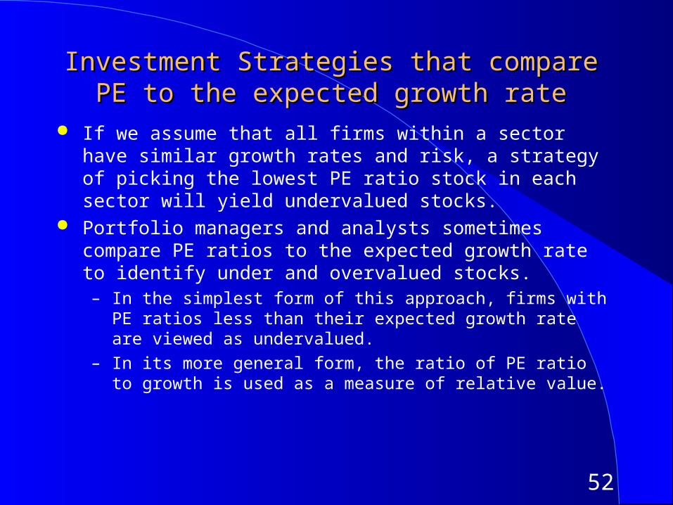
If we assume that all firms within a sector have similar growth rates and risk, a strategy of picking the lowest PE ratio stock in each sector will yield undervalued stocks.

Portfolio managers and analysts sometimes compare PE ratios to the expected growth rate to identify under and overvalued stocks. – In the simplest form of this approach, firms with PE ratios less than their

expected growth rate are viewed as undervalued.

– In its more general form, the ratio of PE ratio to growth is used as a measure of relative value.

53

Problems with comparing PE ratios to Problems with comparing PE ratios to expected growthexpected growth

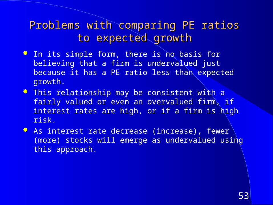
In its simple form, there is no basis for believing that a firm is undervalued just because it has a PE ratio less than expected growth.

This relationship may be consistent with a fairly valued or even an overvalued firm, if interest rates are high, or if a firm is high risk.

As interest rate decrease (increase), fewer (more) stocks will emerge as undervalued using this approach.

54

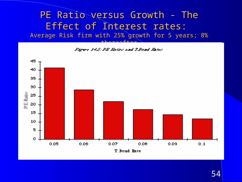
PE Ratio versus Growth - The Effect of Interest PE Ratio versus Growth - The Effect of Interest rates: rates:

Average Risk firm with 25% growth for 5 years; 8% thereafterAverage Risk firm with 25% growth for 5 years; 8% thereafter

55

PE Ratios Less Than The Expected Growth PE Ratios Less Than The Expected Growth RateRate

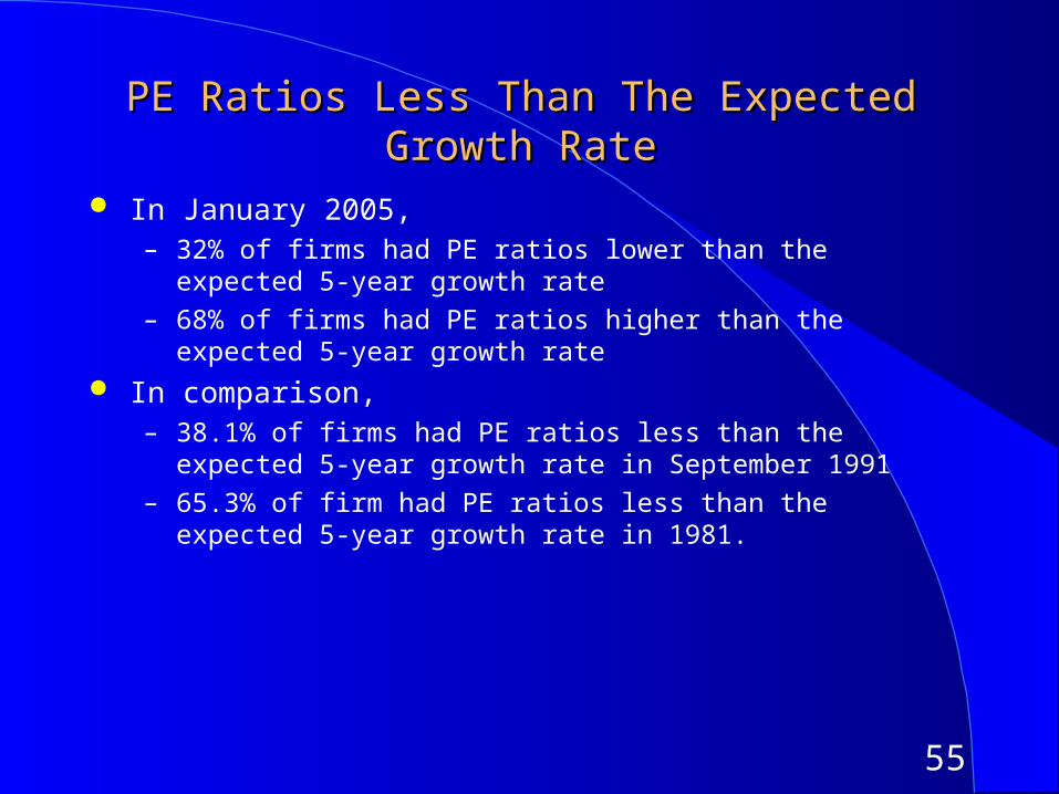
In January 2005,– 32% of firms had PE ratios lower than the expected 5-year growth rate

– 68% of firms had PE ratios higher than the expected 5-year growth rate In comparison,

– 38.1% of firms had PE ratios less than the expected 5-year growth rate in September 1991

– 65.3% of firm had PE ratios less than the expected 5-year growth rate in 1981.

56

PEG Ratio: DefinitionPEG Ratio: Definition

The PEG ratio is the ratio of price earnings to expected growth in earnings per share.

PEG = PE / Expected Growth Rate in Earnings Definitional tests:

– Is the growth rate used to compute the PEG ratio on the same base? (base year EPS) over the same period?(2 years, 5 years) from the same source? (analyst projections, consensus estimates..)

– Is the earnings used to compute the PE ratio consistent with the growth rate estimate?

No double counting: If the estimate of growth in earnings per share is from the current year, it would be a mistake to use forward EPS in computing PE

If looking at foreign stocks or ADRs, is the earnings used for the PE ratio consistent with the growth rate estimate? (US analysts use the ADR EPS)

57

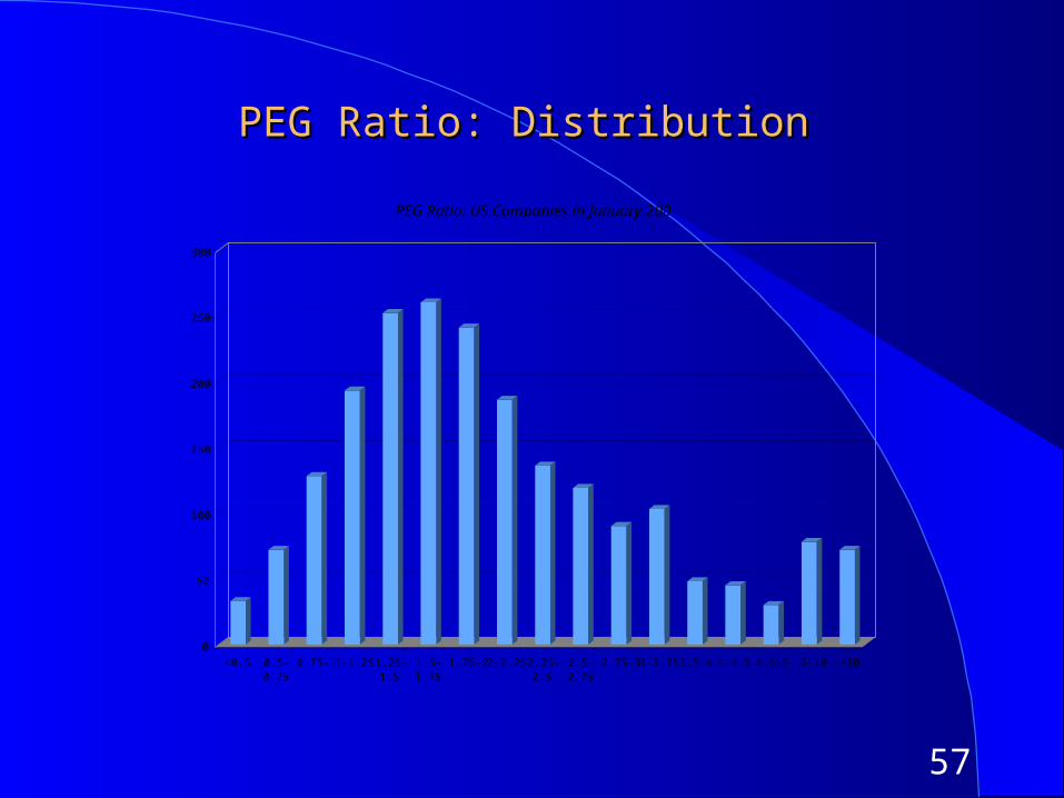
PEG Ratio: DistributionPEG Ratio: Distribution

0

50

100

150

200

250

300

<0.5 0.5-0.75

0.75-1 1-1.25 1.25-1.5

1.5-1.75

1.75-2 2-2.25 2.25-2.5

2.5-2.75

2.75-3 3-3.35 3.5-4 4-4.5 4.5-5 5-10 >10

PEG Ratio: US Companies in January 2005

58

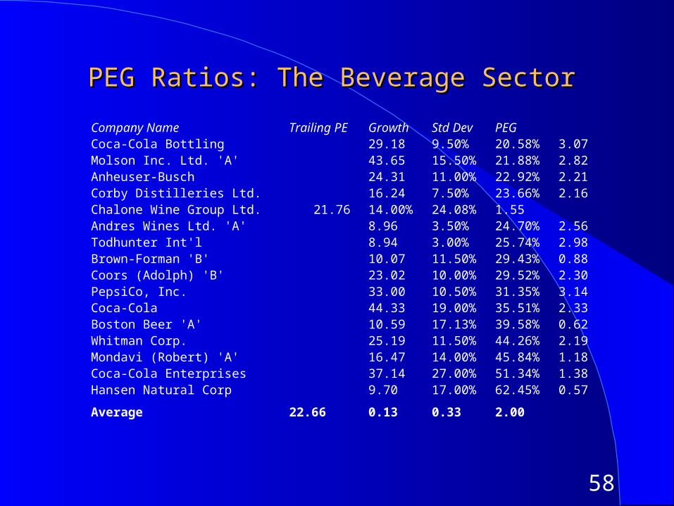
PEG Ratios: The Beverage SectorPEG Ratios: The Beverage Sector

Company Name Trailing PE Growth Std Dev PEGCoca-Cola Bottling 29.18 9.50% 20.58% 3.07Molson Inc. Ltd. 'A' 43.65 15.50% 21.88% 2.82Anheuser-Busch 24.31 11.00% 22.92% 2.21Corby Distilleries Ltd. 16.24 7.50% 23.66% 2.16Chalone Wine Group Ltd. 21.76 14.00% 24.08% 1.55Andres Wines Ltd. 'A' 8.96 3.50% 24.70% 2.56Todhunter Int'l 8.94 3.00% 25.74% 2.98Brown-Forman 'B' 10.07 11.50% 29.43% 0.88Coors (Adolph) 'B' 23.02 10.00% 29.52% 2.30PepsiCo, Inc. 33.00 10.50% 31.35% 3.14Coca-Cola 44.33 19.00% 35.51% 2.33Boston Beer 'A' 10.59 17.13% 39.58% 0.62Whitman Corp. 25.19 11.50% 44.26% 2.19Mondavi (Robert) 'A' 16.47 14.00% 45.84% 1.18Coca-Cola Enterprises 37.14 27.00% 51.34% 1.38Hansen Natural Corp 9.70 17.00% 62.45% 0.57

Average 22.66 0.13 0.33 2.00

59

PEG Ratio: Reading the NumbersPEG Ratio: Reading the Numbers

The average PEG ratio for the beverage sector is 2.00. The lowest PEG ratio in the group belongs to Hansen Natural, which has a PEG ratio of 0.57. Using this measure of value, Hansen Natural is

the most under valued stock in the group the most over valued stock in the group What other explanation could there be for Hansen’s low PEG ratio?

60

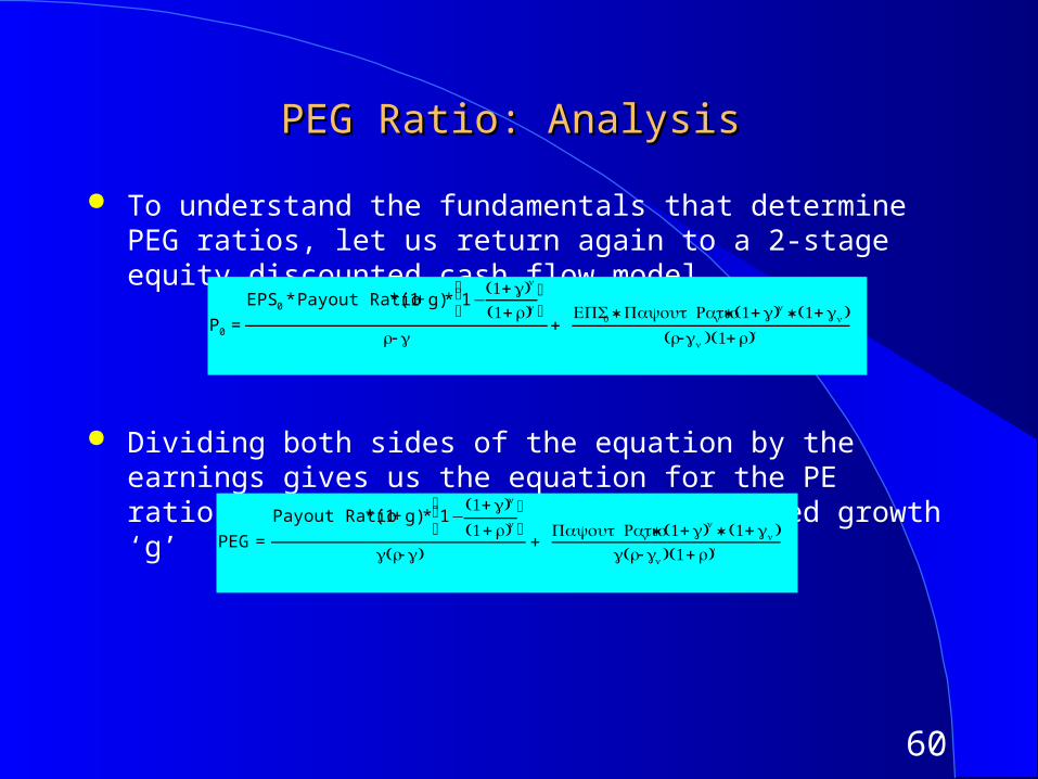
PEG Ratio: AnalysisPEG Ratio: Analysis

To understand the fundamentals that determine PEG ratios, let us return again to a 2-stage equity discounted cash flow model

Dividing both sides of the equation by the earnings gives us the equation for the PE ratio. Dividing it again by the expected growth ‘g’

P0 =

EPS0 * Payout Ratio *(1+ g)* 1−(1+ )g n

(1+ )r n

⎛ ⎝ ⎜ ⎞

⎠

r-g+

EPS0 * Payout Ration * (1+ )g n * (1+gn)(r-gn )(1+ )r n

PEG =

Payout Ratio *(1 + g) * 1−(1+ )g n

(1 + )r n

⎛ ⎝ ⎜ ⎞

⎠(g r- )g

+ Payout Ration * (1+ )g n * (1+gn)(g r-gn)(1 + )r n

61

PEG Ratios and FundamentalsPEG Ratios and Fundamentals

Risk and payout, which affect PE ratios, continue to affect PEG ratios as well.– Implication: When comparing PEG ratios across companies, we are

making implicit or explicit assumptions about these variables. Dividing PE by expected growth does not neutralize the effects of

expected growth, since the relationship between growth and value is not linear and fairly complex (even in a 2-stage model)

62

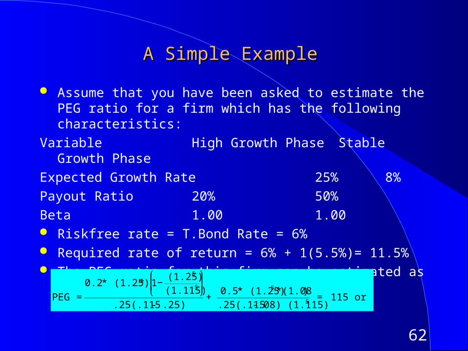
A Simple ExampleA Simple Example

Assume that you have been asked to estimate the PEG ratio for a firm which has the following characteristics:

Variable High Growth Phase Stable Growth Phase

Expected Growth Rate 25% 8%

Payout Ratio 20% 50%

Beta 1.00 1.00 Riskfree rate = T.Bond Rate = 6% Required rate of return = 6% + 1(5.5%)= 11.5% The PEG ratio for this firm can be estimated as follows:

€

PEG =

0.2 * (1.25) * 1−(1.25)5

(1.115)5

⎛

⎝ ⎜

⎞

⎠ ⎟

.25(.115 - .25)+

0.5 * (1.25)5 * (1.08)

.25(.115 - .08) (1.115)5 = 115 or 1.15

63

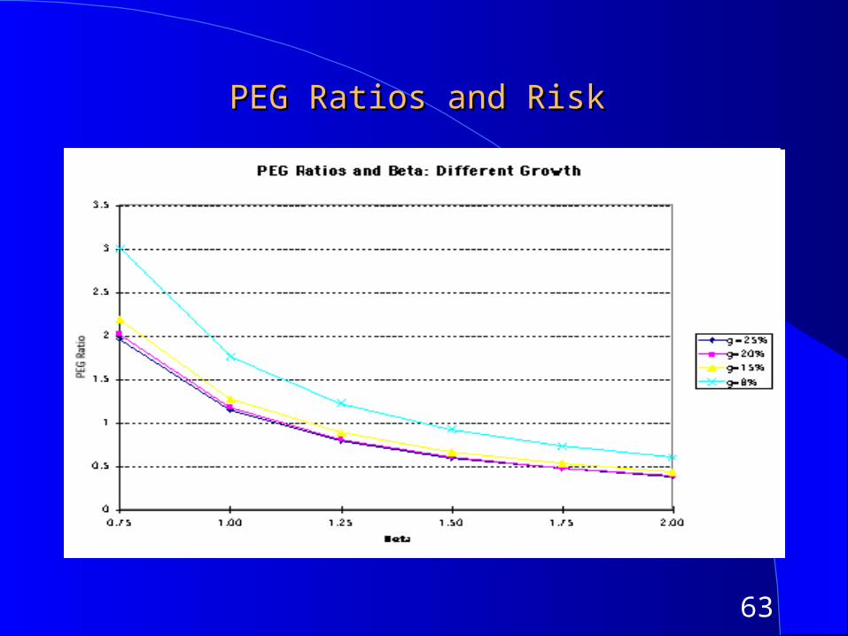
PEG Ratios and RiskPEG Ratios and Risk

64

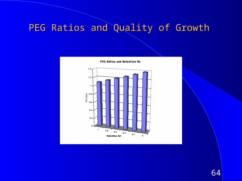
PEG Ratios and Quality of GrowthPEG Ratios and Quality of Growth

65

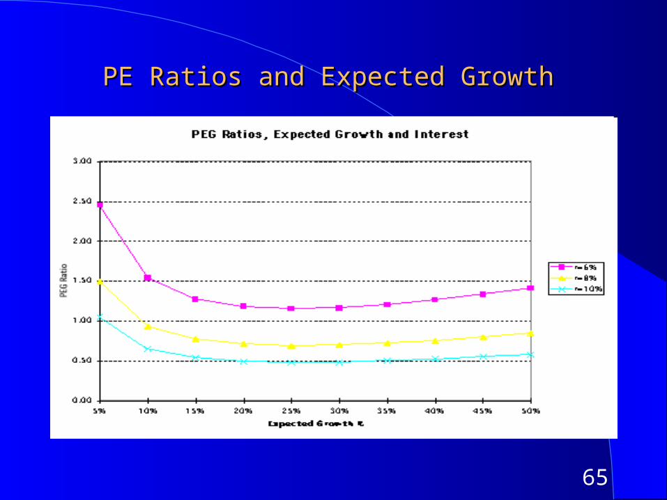
PE Ratios and Expected GrowthPE Ratios and Expected Growth

66

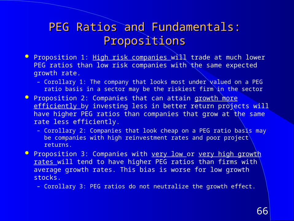
PEG Ratios and Fundamentals: PropositionsPEG Ratios and Fundamentals: Propositions

Proposition 1: High risk companies will trade at much lower PEG ratios than low risk companies with the same expected growth rate.– Corollary 1: The company that looks most under valued on a PEG ratio

basis in a sector may be the riskiest firm in the sector Proposition 2: Companies that can attain growth more efficiently by

investing less in better return projects will have higher PEG ratios than companies that grow at the same rate less efficiently.– Corollary 2: Companies that look cheap on a PEG ratio basis may be

companies with high reinvestment rates and poor project returns. Proposition 3: Companies with very low or very high growth rates will

tend to have higher PEG ratios than firms with average growth rates. This bias is worse for low growth stocks.– Corollary 3: PEG ratios do not neutralize the growth effect.

67

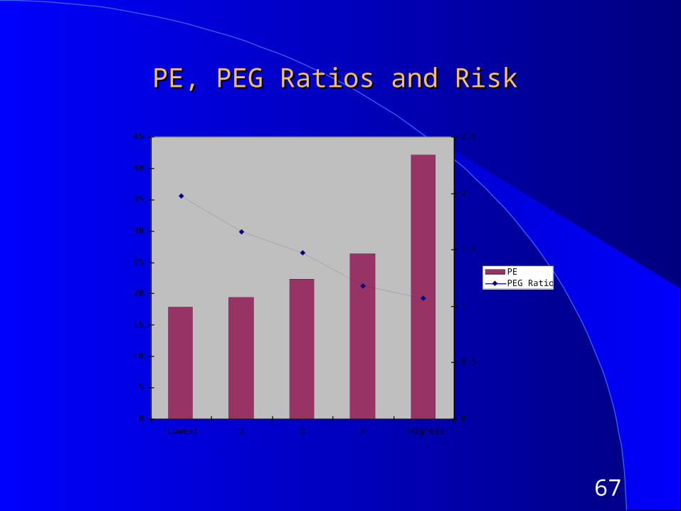
PE, PEG Ratios and RiskPE, PEG Ratios and Risk

0

5

10

15

20

25

30

35

40

45

Lowest 2 3 4 Highest

0

0.5

1

1.5

2

2.5

PEPEG Ratio

68

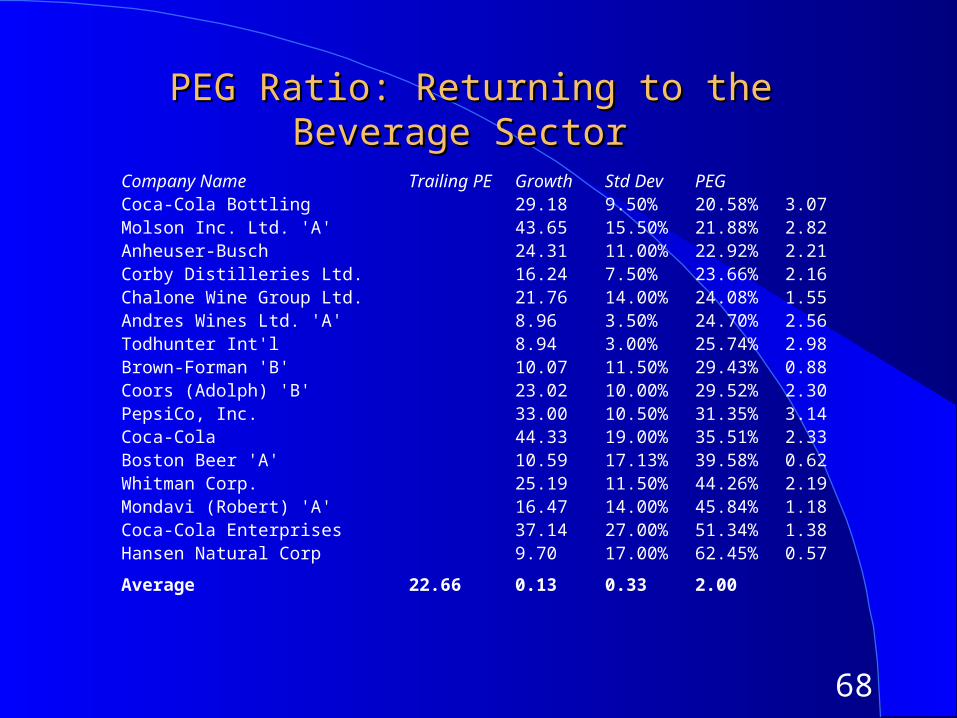
PEG Ratio: Returning to the Beverage Sector PEG Ratio: Returning to the Beverage Sector

Company Name Trailing PE Growth Std Dev PEGCoca-Cola Bottling 29.18 9.50% 20.58% 3.07Molson Inc. Ltd. 'A' 43.65 15.50% 21.88% 2.82Anheuser-Busch 24.31 11.00% 22.92% 2.21Corby Distilleries Ltd. 16.24 7.50% 23.66% 2.16Chalone Wine Group Ltd. 21.76 14.00% 24.08% 1.55Andres Wines Ltd. 'A' 8.96 3.50% 24.70% 2.56Todhunter Int'l 8.94 3.00% 25.74% 2.98Brown-Forman 'B' 10.07 11.50% 29.43% 0.88Coors (Adolph) 'B' 23.02 10.00% 29.52% 2.30PepsiCo, Inc. 33.00 10.50% 31.35% 3.14Coca-Cola 44.33 19.00% 35.51% 2.33Boston Beer 'A' 10.59 17.13% 39.58% 0.62Whitman Corp. 25.19 11.50% 44.26% 2.19Mondavi (Robert) 'A' 16.47 14.00% 45.84% 1.18Coca-Cola Enterprises 37.14 27.00% 51.34% 1.38Hansen Natural Corp 9.70 17.00% 62.45% 0.57

Average 22.66 0.13 0.33 2.00

69

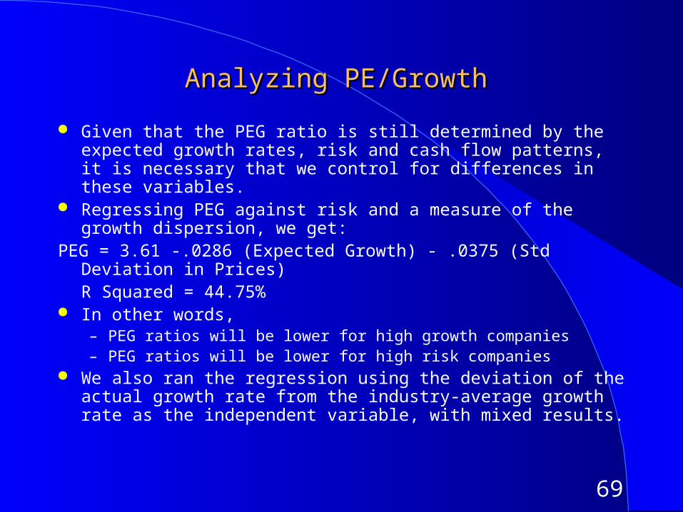
Analyzing PE/GrowthAnalyzing PE/Growth

Given that the PEG ratio is still determined by the expected growth rates, risk and cash flow patterns, it is necessary that we control for differences in these variables.

Regressing PEG against risk and a measure of the growth dispersion, we get:

PEG = 3.61 -.0286 (Expected Growth) - .0375 (Std Deviation in Prices)R Squared = 44.75%

In other words, – PEG ratios will be lower for high growth companies– PEG ratios will be lower for high risk companies

We also ran the regression using the deviation of the actual growth rate from the industry-average growth rate as the independent variable, with mixed results.

70

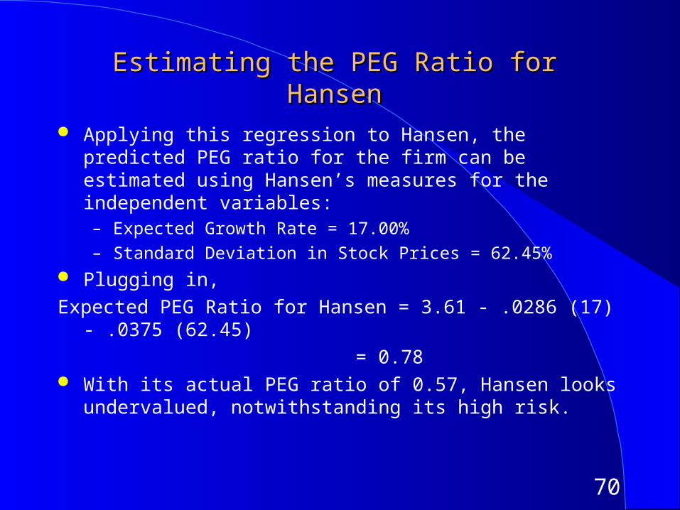
Estimating the PEG Ratio for HansenEstimating the PEG Ratio for Hansen

Applying this regression to Hansen, the predicted PEG ratio for the firm can be estimated using Hansen’s measures for the independent variables:– Expected Growth Rate = 17.00%

– Standard Deviation in Stock Prices = 62.45% Plugging in,

Expected PEG Ratio for Hansen = 3.61 - .0286 (17) - .0375 (62.45)

= 0.78 With its actual PEG ratio of 0.57, Hansen looks undervalued,

notwithstanding its high risk.

71

Extending the ComparablesExtending the Comparables

This analysis, which is restricted to firms in the software sector, can be expanded to include all firms in the firm, as long as we control for differences in risk, growth and payout.

To look at the cross sectional relationship, we first plotted PEG ratios against expected growth rates.

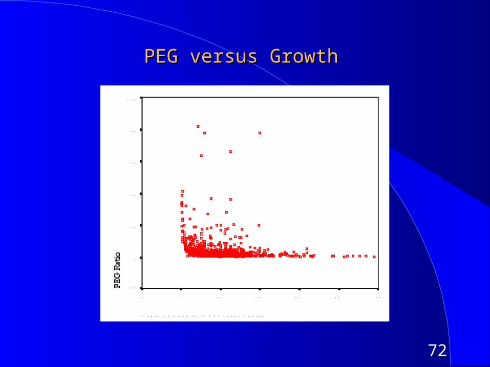
72

PEG versus GrowthPEG versus Growth

E x p e c t e d G r o w t h i n E P S : n e x t 5 y e a r s

1 0 08 06 04 02 00- 2 0

P

E

G

R

a

t

i

o

1 0 0

8 0

6 0

4 0

2 0

0

- 2 0

73

Analyzing the RelationshipAnalyzing the Relationship

The relationship in not linear. In fact, the smallest firms seem to have the highest PEG ratios and PEG ratios become relatively stable at higher growth rates.

To make the relationship more linear, we converted the expected growth rates in ln(expected growth rate). The relationship between PEG ratios and ln(expected growth rate) was then plotted.

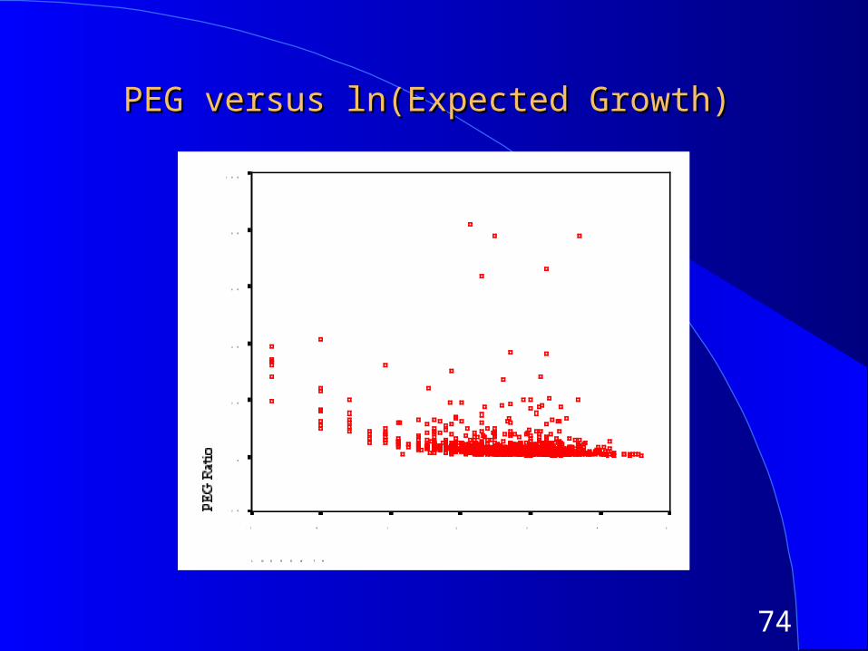
74

PEG versus ln(Expected Growth)PEG versus ln(Expected Growth)

L N G R O W T H

543210- 1

P

E

G

R

a

t

i

o

1 0 0

8 0

6 0

4 0

2 0

0

- 2 0

75

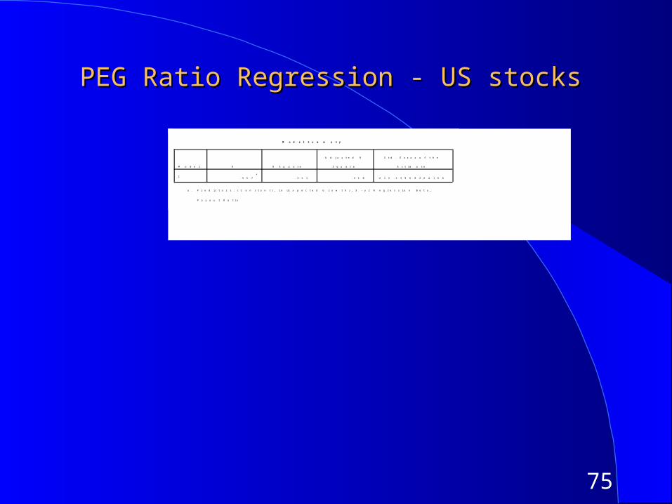
PEG Ratio Regression - US stocksPEG Ratio Regression - US stocks

M o d e l S u m m a r y

. 5 5 7

a

. 3 1 1 . 3 1 0 2 1 3 . 1 5 9 6 8 2 2 4 1 6 6

M o d e l

1

R R S q u a r e

A d j u s t e d R

S q u a r e

S t d . E r r o r o f t h e

E s t i m a t e

P r e d i c t o r s : ( C o n s t a n t ) , l n ( E x p e c t e d G r o w t h ) , 3 - y r R e g r e s s i o n B e t a ,

P a y o u t R a t i o

a .

76

Applying the PEG ratio regressionApplying the PEG ratio regression

Consider Dell again. The stock has an expected growth rate of 10%, a beta of 1.20 and pays out no dividends. What should its PEG ratio be?

If the stock’s actual PE ratio is 22, what does this analysis tell you about the stock?

77

A Variant on PEG Ratio: The PEGY ratioA Variant on PEG Ratio: The PEGY ratio

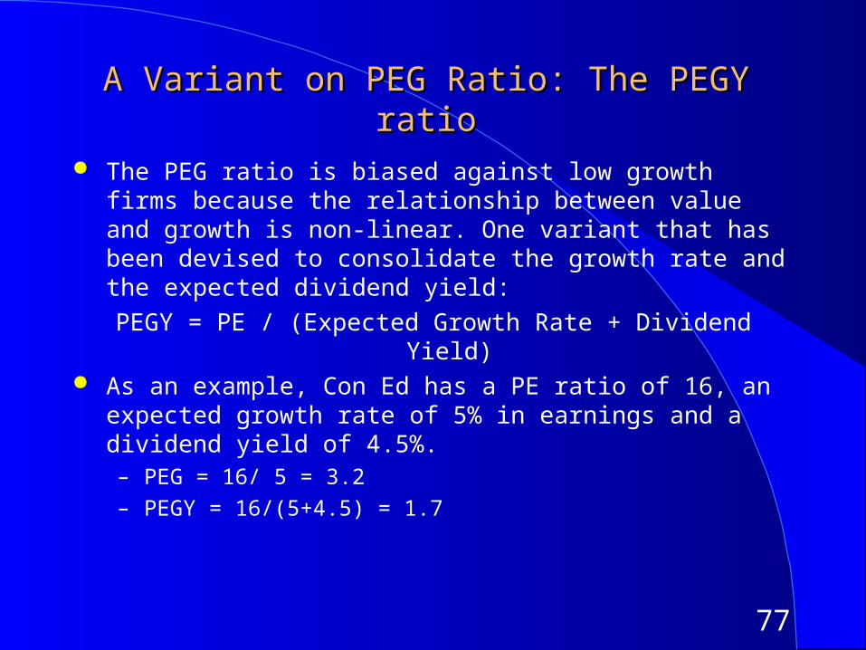
The PEG ratio is biased against low growth firms because the relationship between value and growth is non-linear. One variant that has been devised to consolidate the growth rate and the expected dividend yield:

PEGY = PE / (Expected Growth Rate + Dividend Yield) As an example, Con Ed has a PE ratio of 16, an expected growth rate

of 5% in earnings and a dividend yield of 4.5%.– PEG = 16/ 5 = 3.2

– PEGY = 16/(5+4.5) = 1.7

78

Relative PE: DefinitionRelative PE: Definition

The relative PE ratio of a firm is the ratio of the PE of the firm to the PE of the market.

Relative PE = PE of Firm / PE of Market While the PE can be defined in terms of current earnings, trailing

earnings or forward earnings, consistency requires that it be estimated using the same measure of earnings for both the firm and the market.

Relative PE ratios are usually compared over time. Thus, a firm or sector which has historically traded at half the market PE (Relative PE = 0.5) is considered over valued if it is trading at a relative PE of 0.7.

Relative PE ratios are also used when comparing companies across markets with different PE ratios (Japanese versus US stocks, for example).

79

Relative PE: DeterminantsRelative PE: Determinants

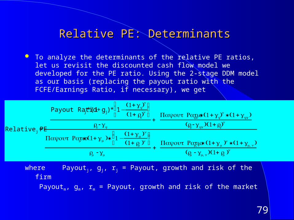
To analyze the determinants of the relative PE ratios, let us revisit the discounted cash flow model we developed for the PE ratio. Using the 2-stage DDM model as our basis (replacing the payout ratio with the FCFE/Earnings Ratio, if necessary), we get

where Payoutj, gj, rj = Payout, growth and risk of the firm

Payoutm, gm, rm = Payout, growth and risk of the market

Relative PE j =

Payout Ratio j *(1 + g j) * 1−(1+gj)

n

(1+ rj)n

⎛

⎝ ⎜ ⎞

⎠ ⎟

rj -gj

+ Payout Ratio,j n * (1 +gj)

n * (1 +g ,j n)(rj -g ,j n)(1 + rj)

n

Payout Ratiom* (1+gm)* 1−(1+gm)

n

(1+ rm)n

⎛ ⎝ ⎜ ⎞

⎠ ⎟

rm -gm

+ Payout Ratio,mn * (1+gm)

n * (1 +g ,m n)(rm- g ,m n)(1+ rm)

n

80

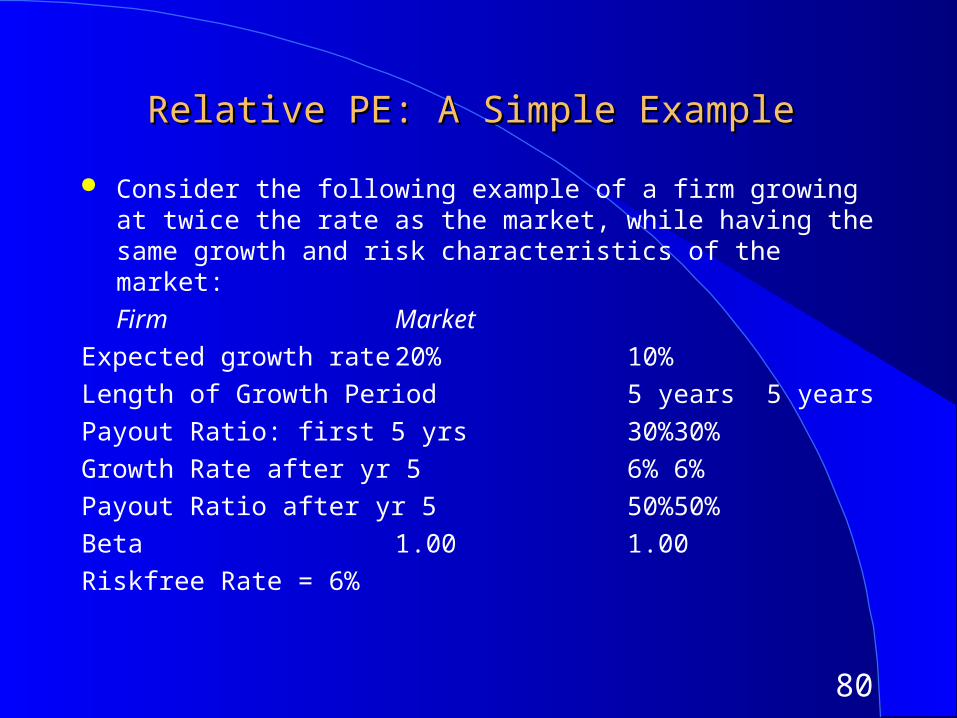
Relative PE: A Simple ExampleRelative PE: A Simple Example

Consider the following example of a firm growing at twice the rate as the market, while having the same growth and risk characteristics of the market:

Firm Market

Expected growth rate 20% 10%

Length of Growth Period 5 years 5 years

Payout Ratio: first 5 yrs 30% 30%

Growth Rate after yr 5 6% 6%

Payout Ratio after yr 5 50% 50%

Beta 1.00 1.00

Riskfree Rate = 6%

81

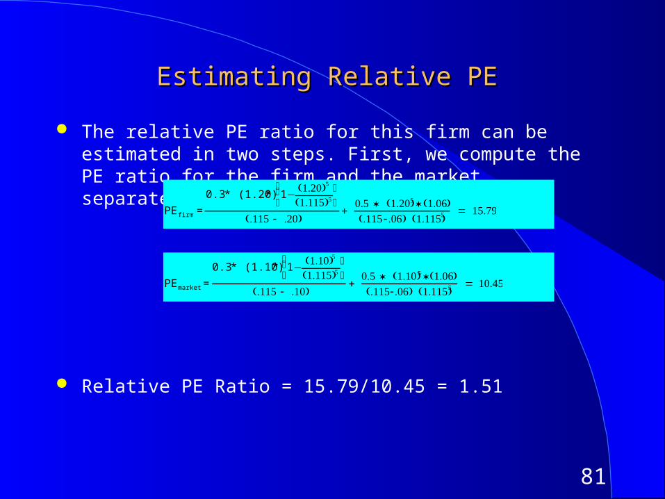
Estimating Relative PEEstimating Relative PE

The relative PE ratio for this firm can be estimated in two steps. First, we compute the PE ratio for the firm and the market separately:

Relative PE Ratio = 15.79/10.45 = 1.51

PE firm =

0.3 * (1.20) * 1− (1.20)5

(1.115)5 ⎛ ⎝ ⎜ ⎞

⎠(.115 - .20)

+ 0.5 * (1.20)5 * (1.06)(.115 -.06) (1.115)5

= 15.79

PEmarket =

0.3 * (1.10) * 1− (1.10)5

(1.115)5 ⎛ ⎝ ⎜ ⎞

⎠(.115 - .10)

+ 0.5 * (1.10)5 * (1.06)(.115-.06) (1.115)5

= 10.45

82

Relative PE and Relative GrowthRelative PE and Relative Growth

83

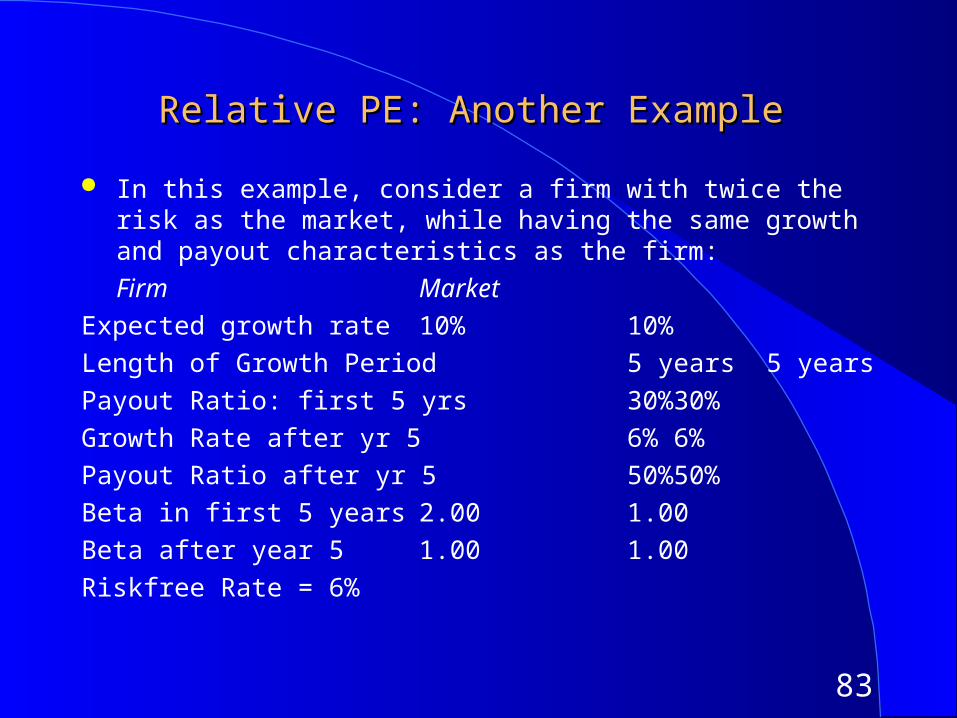
Relative PE: Another ExampleRelative PE: Another Example

In this example, consider a firm with twice the risk as the market, while having the same growth and payout characteristics as the firm:

Firm Market

Expected growth rate 10% 10%

Length of Growth Period 5 years 5 years

Payout Ratio: first 5 yrs 30% 30%

Growth Rate after yr 5 6% 6%

Payout Ratio after yr 5 50% 50%

Beta in first 5 years 2.00 1.00

Beta after year 5 1.00 1.00

Riskfree Rate = 6%

84

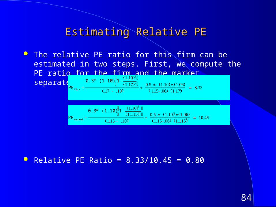
Estimating Relative PEEstimating Relative PE

The relative PE ratio for this firm can be estimated in two steps. First, we compute the PE ratio for the firm and the market separately:

Relative PE Ratio = 8.33/10.45 = 0.80

PE firm =

0.3 * (1.10) * 1−(1.10)5

(1.17)5 ⎛ ⎝ ⎜ ⎞

⎠(.17 - .10)

+ 0.5 * (1.10)5 * (1.06)(.115- .06) (1.17)5

= 8.33

PEmarket =

0.3 * (1.10) * 1− (1.10)5

(1.115)5 ⎛ ⎝ ⎜ ⎞

⎠(.115 - .10)

+ 0.5 * (1.10)5 * (1.06)(.115-.06) (1.115)5

= 10.45

85

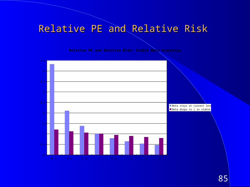
Relative PE and Relative RiskRelative PE and Relative Risk

Relative PE and Relative Risk: Stable Beta Scenarios

0

0.5

1

1.5

2

2.5

3

3.5

4

4.5

0.25 0.5 0.75 1 1.25 1.5 1.75 2

Beta stays at current levelBeta drops to 1 in stable phase

86

Relative PE: Summary of DeterminantsRelative PE: Summary of Determinants

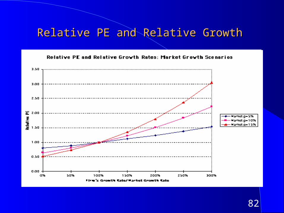
The relative PE ratio of a firm is determined by two variables. In particular, it will– increase as the firm’s growth rate relative to the market increases. The

rate of change in the relative PE will itself be a function of the market growth rate, with much greater changes when the market growth rate is higher. In other words, a firm or sector with a growth rate twice that of the market will have a much higher relative PE when the market growth rate is 10% than when it is 5%.

– decrease as the firm’s risk relative to the market increases. The extent of the decrease depends upon how long the firm is expected to stay at this level of relative risk. If the different is permanent, the effect is much greater.

Relative PE ratios seem to be unaffected by the level of rates, which might give them a decided advantage over PE ratios.

87

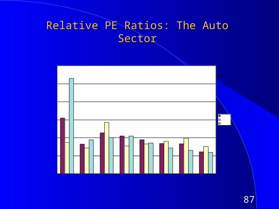
Relative PE Ratios: The Auto SectorRelative PE Ratios: The Auto Sector

Relative PE Ratios: Auto Stocks

0.00

0.20

0.40

0.60

0.80

1.00

1.20

1993 1994 1995 1996 1997 1998 1999 2000

Ford

Chrysler

GM

88

Using Relative PE ratiosUsing Relative PE ratios

On a relative PE basis, all of the automobile stocks looked cheap in 2000 because they were trading at their lowest relative PE ratios than 1993. Why might the relative PE ratio be lower in 2000 than in 1993?

89

Relative PE Ratios: US stocksRelative PE Ratios: US stocks

M o d e l S u m m a r y

. 5 0 2

a

. 2 5 2 . 2 5 1 4 9 . 2 2 8 3 8

M o d e l

1

R R S q u a r e

A d j u s t e d R

S q u a r e

S t d . E r r o r o f

t h e E s t i m a t e

P r e d i c t o r s : ( C o n s t a n t ) , 3 - y r R e g r e s s i o n B e t a , R e l a t i v e G r o w t ha .

90

Value/Earnings and Value/Cashflow RatiosValue/Earnings and Value/Cashflow Ratios

While Price earnings ratios look at the market value of equity relative to earnings to equity investors, Value earnings ratios look at the market value of the operating assets of the firm (Enterprise value or EV) relative to operating earnings or cash flows.

The form of value to cash flow ratios that has the closest parallels in DCF valuation is the value to Free Cash Flow to the Firm, which is defined as:

EV/FCFF = (Market Value of Equity + Market Value of Debt-Cash)

EBIT (1-t) - (Cap Ex - Deprecn) - Chg in Working Cap

91

Value of Firm/FCFF: DeterminantsValue of Firm/FCFF: Determinants

Reverting back to a two-stage FCFF DCF model, we get:

– V0 = Value of the firm (today)

– FCFF0 = Free Cashflow to the firm in current year

– g = Expected growth rate in FCFF in extraordinary growth period (first n years)

– WACC = Weighted average cost of capital

– gn = Expected growth rate in FCFF in stable growth period (after n years)

V0 =

FCFF0 (1 + g) 1-

(1 + g)n

(1+ WACC)n

⎛

⎝ ⎜

⎞

⎠ ⎟

WACC -g +

FCFF0 (1+ )g n(1+gn)

(WACC -gn)(1 + )WACC n

92

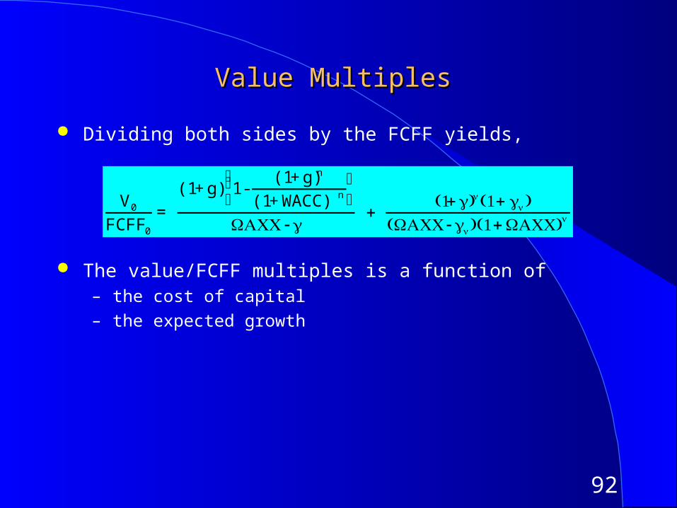
Value MultiplesValue Multiples

Dividing both sides by the FCFF yields,

The value/FCFF multiples is a function of– the cost of capital

– the expected growth

V0

FCFF0

=

(1 + g) 1-(1 + g)n

(1 + WACC) n

⎛ ⎝ ⎜ ⎞

⎠WACC -g

+ (1+ )g n(1+ gn)

(WACC -gn)(1 + )WACC n

93

Alternatives to FCFF - EBIT and EBITDAAlternatives to FCFF - EBIT and EBITDA

Most analysts find FCFF to complex or messy to use in multiples (partly because capital expenditures and working capital have to be estimated). They use modified versions of the multiple with the following alternative denominator:– after-tax operating income or EBIT(1-t)

– pre-tax operating income or EBIT

– net operating income (NOI), a slightly modified version of operating income, where any non-operating expenses and income is removed from the EBIT

– EBITDA, which is earnings before interest, taxes, depreciation and amortization.

94

Value/FCFF Multiples and the AlternativesValue/FCFF Multiples and the Alternatives

Assume that you have computed the value of a firm, using discounted cash flow models. Rank the following multiples in the order of magnitude from lowest to highest?

Value/EBIT Value/EBIT(1-t) Value/FCFF Value/EBITDA What assumption(s) would you need to make for the Value/EBIT(1-t)

ratio to be equal to the Value/FCFF multiple?

95

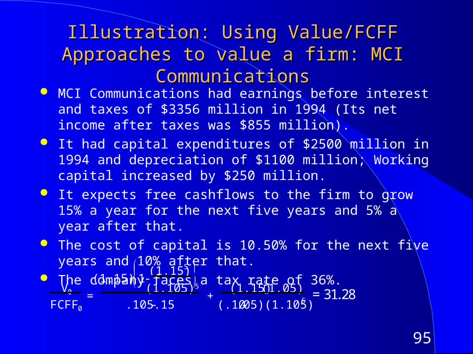
Illustration: Using Value/FCFF Approaches to Illustration: Using Value/FCFF Approaches to value a firm: MCI Communicationsvalue a firm: MCI Communications

MCI Communications had earnings before interest and taxes of $3356 million in 1994 (Its net income after taxes was $855 million).

It had capital expenditures of $2500 million in 1994 and depreciation of $1100 million; Working capital increased by $250 million.

It expects free cashflows to the firm to grow 15% a year for the next five years and 5% a year after that.

The cost of capital is 10.50% for the next five years and 10% after that.

The company faces a tax rate of 36%.

V0

FCFF0

=

(1.15) 1-(1.15)5

(1.105)5

.105 -.15 +

(1.15)5(1.05)

(.10 - .05)(1.105)5 = 31.28

96

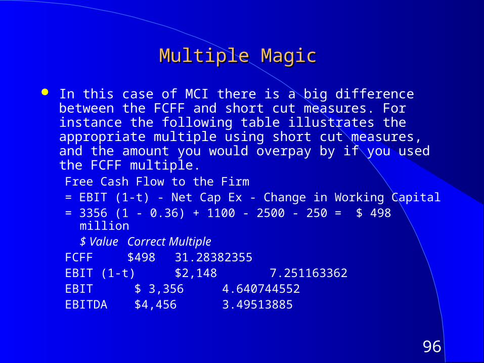
Multiple MagicMultiple Magic

In this case of MCI there is a big difference between the FCFF and short cut measures. For instance the following table illustrates the appropriate multiple using short cut measures, and the amount you would overpay by if you used the FCFF multiple.Free Cash Flow to the Firm = EBIT (1-t) - Net Cap Ex - Change in Working Capital= 3356 (1 - 0.36) + 1100 - 2500 - 250 = $ 498 million

$ Value Correct MultipleFCFF $498 31.28382355EBIT (1-t) $2,148 7.251163362EBIT $ 3,356 4.640744552EBITDA $4,456 3.49513885

97

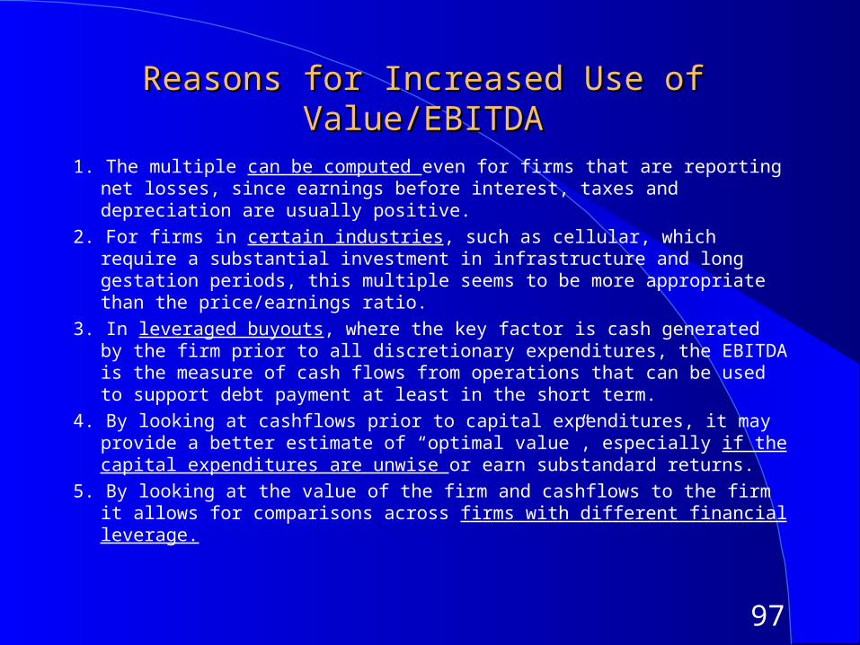
Reasons for Increased Use of Value/EBITDAReasons for Increased Use of Value/EBITDA

1. The multiple can be computed even for firms that are reporting net losses, since earnings before interest, taxes and depreciation are usually positive.

2. For firms in certain industries, such as cellular, which require a substantial investment in infrastructure and long gestation periods, this multiple seems to be more appropriate than the price/earnings ratio.

3. In leveraged buyouts, where the key factor is cash generated by the firm prior to all discretionary expenditures, the EBITDA is the measure of cash flows from operations that can be used to support debt payment at least in the short term.

4. By looking at cashflows prior to capital expenditures, it may provide a better estimate of “optimal value”, especially if the capital expenditures are unwise or earn substandard returns.

5. By looking at the value of the firm and cashflows to the firm it allows for comparisons across firms with different financial leverage.

98

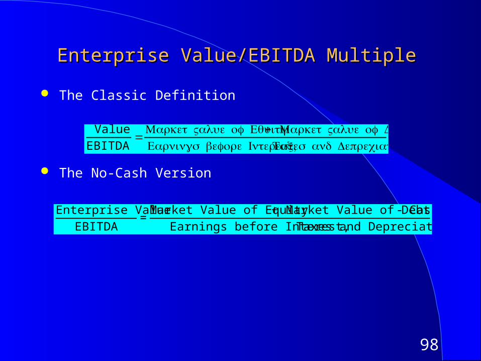
Enterprise Value/EBITDA MultipleEnterprise Value/EBITDA Multiple

The Classic Definition

The No-Cash Version

Value

EBITDA=

Market Value of Equity+ Market Value of Debt ,Earnings before Interest Taxes and Depreciation

€

Enterprise ValueEBITDA

=Market Value of Equity + Market Value of Debt - Cash

Earnings before Interest, Taxes and Depreciation

99

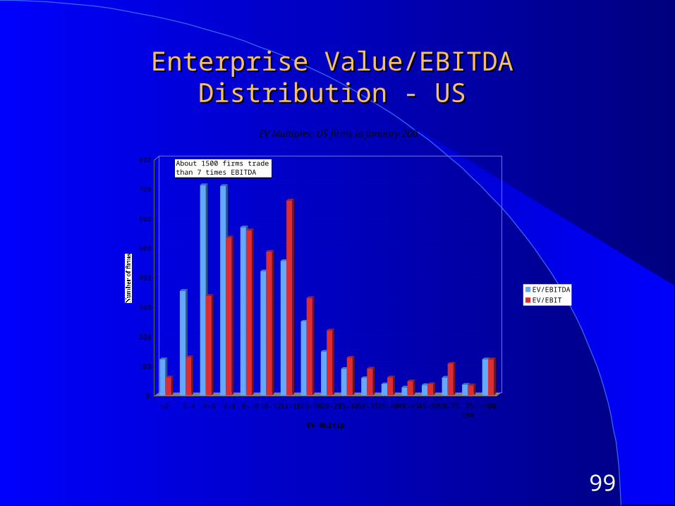
Enterprise Value/EBITDA Distribution - USEnterprise Value/EBITDA Distribution - US

0

100

200

300

400

500

600

700

800

Number of firms

<2 2-4 4-6 6-8 8-10 10-12 12-16 16-20 20-25 25-30 30-35 35-40 40-45 45-50 50-75 75-100

>100

EV Multiple

EV Multiples: US firms in January 2005

EV/EBITDA

EV/EBIT

About 1500 firms trade at less than 7 times EBITDA

100

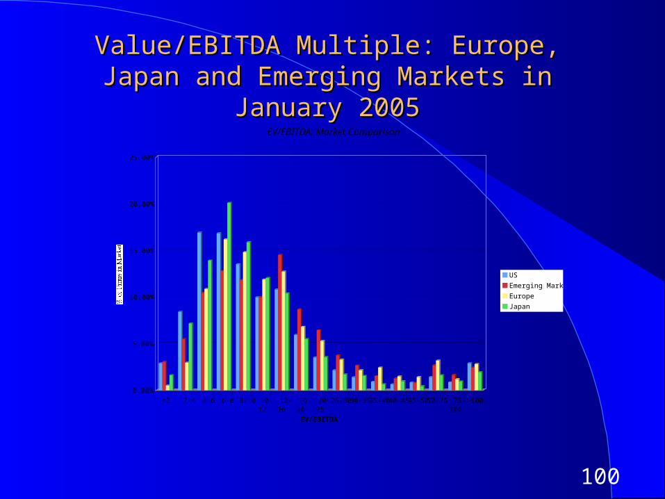
Value/EBITDA Multiple: Europe, Japan and Value/EBITDA Multiple: Europe, Japan and Emerging Markets in January 2005Emerging Markets in January 2005

0.00%

5.00%

10.00%

15.00%

20.00%

25.00%

% of Firms in Market

<2 2-4 4-6 6-8 8-10 10-12

12-16

16-20

20-25

25-30 30-35 35-40 40-45 45-50 50-75 75-100

>100

EV/EBITDA

EV/EBITDA: Market Comparison

US

Emerging Markets

Europe

Japan

101

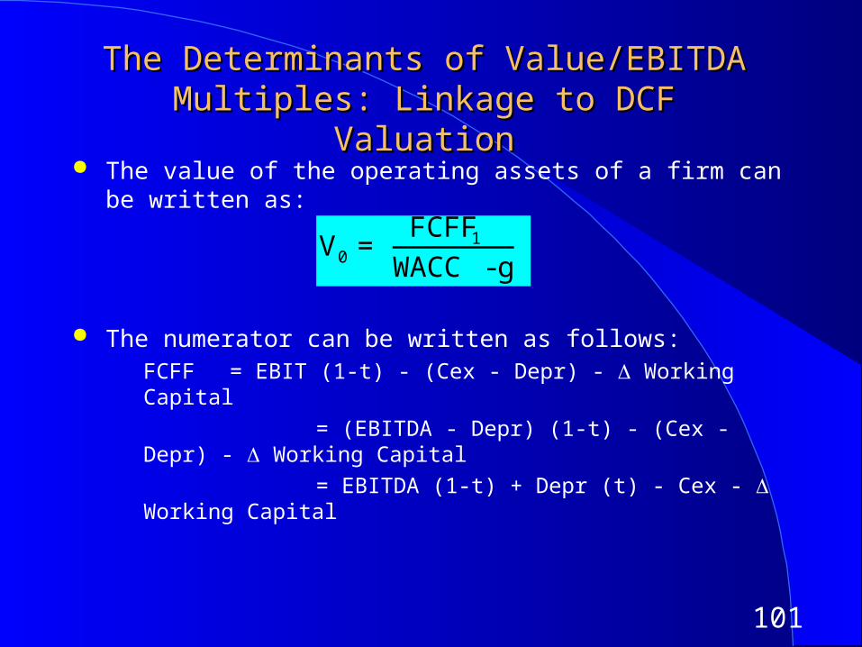
The Determinants of Value/EBITDA Multiples: The Determinants of Value/EBITDA Multiples: Linkage to DCF ValuationLinkage to DCF Valuation

The value of the operating assets of a firm can be written as:

The numerator can be written as follows:FCFF = EBIT (1-t) - (Cex - Depr) - Working Capital

= (EBITDA - Depr) (1-t) - (Cex - Depr) - Working Capital

= EBITDA (1-t) + Depr (t) - Cex - Working Capital

V0 = FCFF1

WACC - g

102

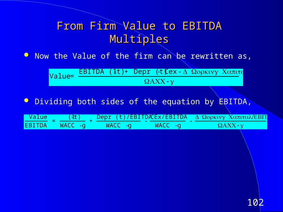
From Firm Value to EBITDA MultiplesFrom Firm Value to EBITDA Multiples

Now the Value of the firm can be rewritten as,

Dividing both sides of the equation by EBITDA,

Value = EBITDA (1 - t) + Depr (t) - Cex - Working Capital

WACC -g

Value

EBITDA =

(1- t)

WACC - g +

Depr (t)/EBITDA

WACC -g -

CEx/EBITDA

WACC - g -

/Working Capital EBITDAWACC -g

103

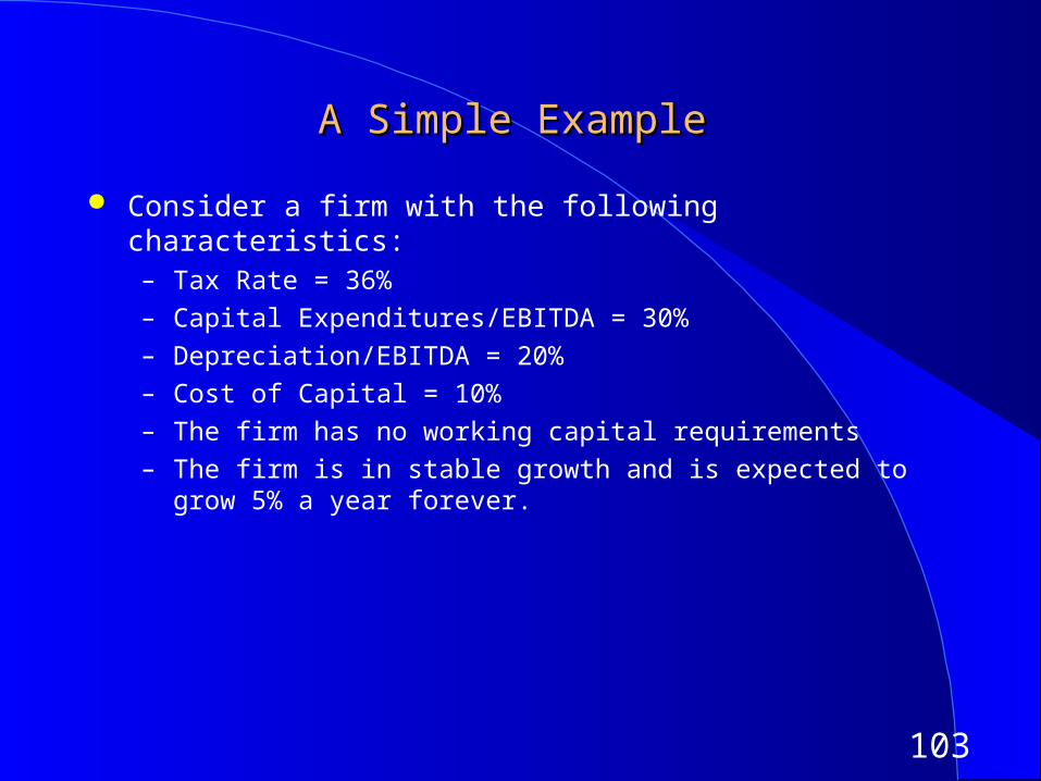
A Simple ExampleA Simple Example

Consider a firm with the following characteristics:– Tax Rate = 36%

– Capital Expenditures/EBITDA = 30%

– Depreciation/EBITDA = 20%

– Cost of Capital = 10%

– The firm has no working capital requirements

– The firm is in stable growth and is expected to grow 5% a year forever.

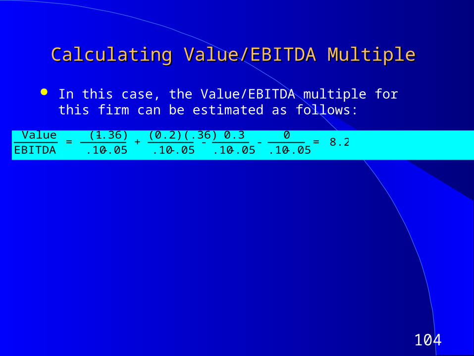
104

Calculating Value/EBITDA MultipleCalculating Value/EBITDA Multiple

In this case, the Value/EBITDA multiple for this firm can be estimated as follows:

Value

EBITDA =

(1- .36)

.10 -.05 +

(0.2)(.36)

.10 -.05 -

0.3

.10 - .05 -

0

.10 - .05 = 8.24

105

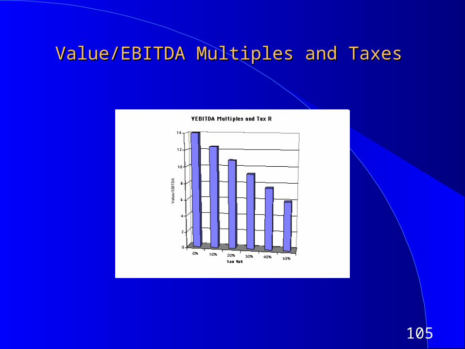
Value/EBITDA Multiples and TaxesValue/EBITDA Multiples and Taxes

106

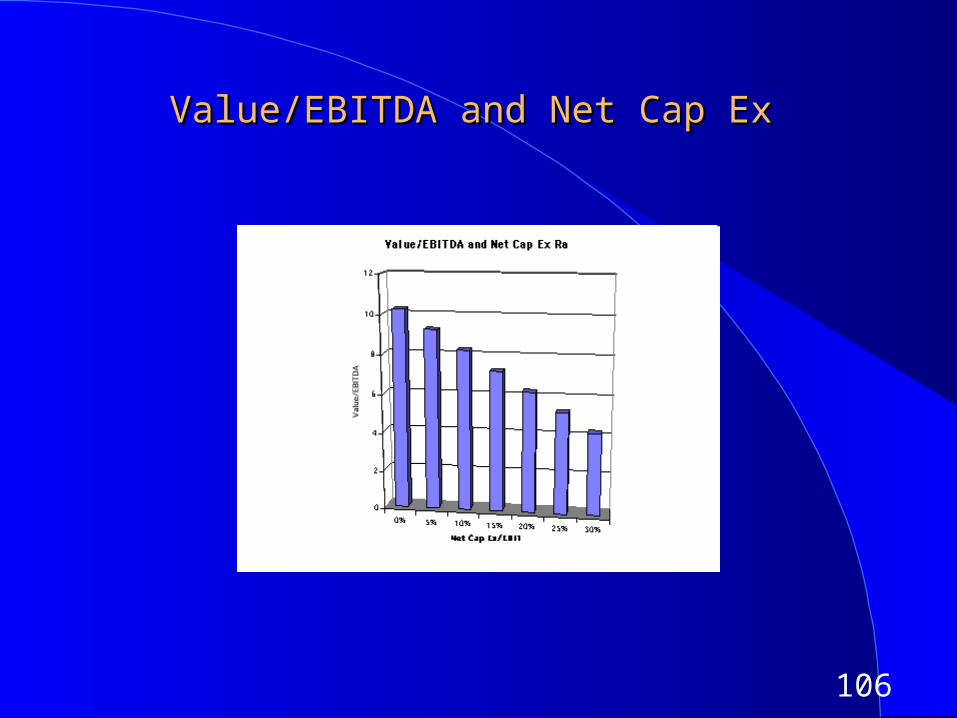
Value/EBITDA and Net Cap ExValue/EBITDA and Net Cap Ex

107

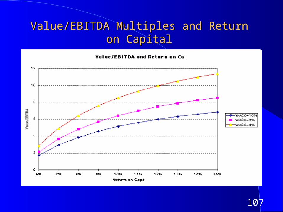
Value/EBITDA Multiples and Return on CapitalValue/EBITDA Multiples and Return on Capital

108

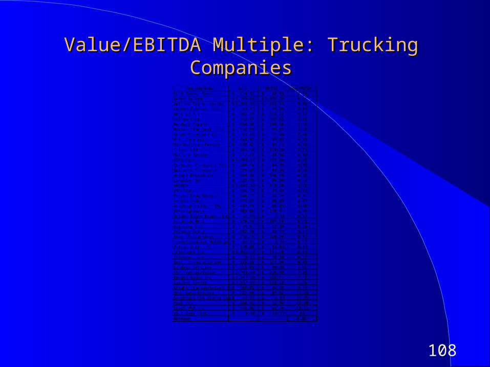
Value/EBITDA Multiple: Trucking CompaniesValue/EBITDA Multiple: Trucking Companies

Company Name Value EBITDA Value/EBITDAKLLM Trans. Svcs. 114.32$ 48.81$ 2.34Ryder System 5,158.04$ 1,838.26$ 2.81Rollins Truck Leasing 1,368.35$ 447.67$ 3.06Cannon Express Inc. 83.57$ 27.05$ 3.09Hunt (J.B.) 982.67$ 310.22$ 3.17Yellow Corp. 931.47$ 292.82$ 3.18Roadway Express 554.96$ 169.38$ 3.28Marten Transport Ltd. 116.93$ 35.62$ 3.28Kenan Transport Co. 67.66$ 19.44$ 3.48M.S. Carriers 344.93$ 97.85$ 3.53Old Dominion Freight 170.42$ 45.13$ 3.78Trimac Ltd 661.18$ 174.28$ 3.79Matlack Systems 112.42$ 28.94$ 3.88XTRA Corp. 1,708.57$ 427.30$ 4.00Covenant Transport Inc 259.16$ 64.35$ 4.03Builders Transport 221.09$ 51.44$ 4.30Werner Enterprises 844.39$ 196.15$ 4.30Landstar Sys. 422.79$ 95.20$ 4.44AMERCO 1,632.30$ 345.78$ 4.72USA Truck 141.77$ 29.93$ 4.74Frozen Food Express 164.17$ 34.10$ 4.81Arnold Inds. 472.27$ 96.88$ 4.87Greyhound Lines Inc. 437.71$ 89.61$ 4.88USFreightways 983.86$ 198.91$ 4.95Golden Eagle Group Inc. 12.50$ 2.33$ 5.37Arkansas Best 578.78$ 107.15$ 5.40Airlease Ltd. 73.64$ 13.48$ 5.46Celadon Group 182.30$ 32.72$ 5.57Amer. Freightways 716.15$ 120.94$ 5.92Transfinancial Holdings 56.92$ 8.79$ 6.47Vitran Corp. 'A' 140.68$ 21.51$ 6.54Interpool Inc. 1,002.20$ 151.18$ 6.63Intrenet Inc. 70.23$ 10.38$ 6.77Swift Transportation 835.58$ 121.34$ 6.89Landair Services 212.95$ 30.38$ 7.01CNF Transportation 2,700.69$ 366.99$ 7.36Budget Group Inc 1,247.30$ 166.71$ 7.48Caliber System 2,514.99$ 333.13$ 7.55Knight Transportation Inc 269.01$ 28.20$ 9.54Heartland Express 727.50$ 64.62$ 11.26Greyhound CDA Transn Corp 83.25$ 6.99$ 11.91Mark VII 160.45$ 12.96$ 12.38Coach USA Inc 678.38$ 51.76$ 13.11US 1 Inds Inc. 5.60$ (0.17)$ NAAverage 5.61

109

A Test on EBITDAA Test on EBITDA

Ryder System looks very cheap on a Value/EBITDA multiple basis, relative to the rest of the sector. What explanation (other than misvaluation) might there be for this difference?

110

Analyzing the Value/EBITDA MultipleAnalyzing the Value/EBITDA Multiple

While low value/EBITDA multiples may be a symptom of undervaluation, a few questions need to be answered:– Is the operating income next year expected to be significantly lower than

the EBITDA for the most recent period? (Price may have dropped)

– Does the firm have significant capital expenditures coming up? (In the trucking business, the life of the trucking fleet would be a good indicator)

– Does the firm have a much higher cost of capital than other firms in the sector?

– Does the firm face a much higher tax rate than other firms in the sector?

111

Value/EBITDA Multiples: MarketValue/EBITDA Multiples: Market

The multiple of value to EBITDA varies widely across firms in the market, depending upon:– how capital intensive the firm is (high capital intensity firms will tend to

have lower value/EBITDA ratios), and how much reinvestment is needed to keep the business going and create growth

– how high or low the cost of capital is (higher costs of capital will lead to lower Value/EBITDA multiples)

– how high or low expected growth is in the sector (high growth sectors will tend to have higher Value/EBITDA multiples)

112

US Market: Cross Sectional RegressionUS Market: Cross Sectional RegressionJanuary 2005January 2005

113

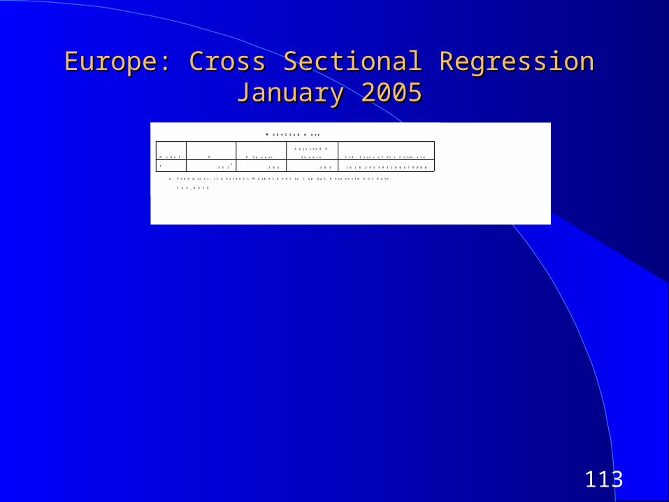
Europe: Cross Sectional RegressionEurope: Cross Sectional RegressionJanuary 2005January 2005

M o d e l S u m m a r y

. 5 5 1a

. 3 0 4 . 3 0 3 1 6 1 8 . 3 9 3 5 9 4 2 0 0 6 7 9 0 0 0

M o d e l

1

R R S q u a r e

A d j u s t e d R

S q u a r e S t d . E r r o r o f t h e E s t i m a t e

P r e d i c t o r s : ( C o n s t a n t ) , M a r k e t D e b t t o C a p i t a l , R e i n v e s t m e n t R a t e ,

T A X _ R A T E

a .

114

Price-Book Value Ratio: DefinitionPrice-Book Value Ratio: Definition

The price/book value ratio is the ratio of the market value of equity to the book value of equity, i.e., the measure of shareholders’ equity in the balance sheet.

Price/Book Value = Market Value of Equity

Book Value of Equity Consistency Tests:

– If the market value of equity refers to the market value of equity of common stock outstanding, the book value of common equity should be used in the denominator.

– If there is more that one class of common stock outstanding, the market values of all classes (even the non-traded classes) needs to be factored in.

115

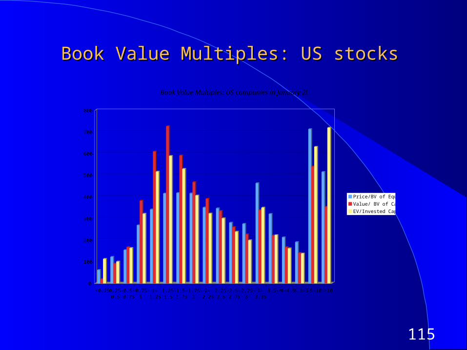
Book Value Multiples: US stocksBook Value Multiples: US stocks

0

100

200

300

400

500

600

700

800

<0.25 0.25-0.5

0.5-0.75

0.75-1

1-1.25

1.25-1.5

1.5-1.75

1.75-2

2-2.25

2.25-2.5

2.5-2.75

2.75-3

3-3.35

3.5-4 4-4.5 4.5-5 5-10 >10

Book Value Multiples: US companies in January 2005

Price/BV of Equity

Value/ BV of Capital

EV/Invested Capital

116

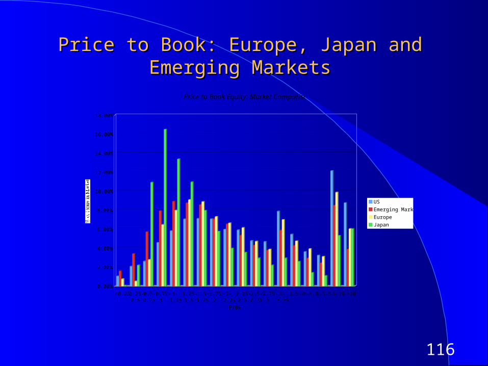
Price to Book: Europe, Japan and Emerging Price to Book: Europe, Japan and Emerging MarketsMarkets

0.00%

2.00%

4.00%

6.00%

8.00%

10.00%

12.00%

14.00%

16.00%

18.00%

% of Firms in Market

<0.25 0.25-0.5

0.5-0.75

0.75-1

1-1.25

1.25-1.5

1.5-1.75

1.75-2

2-2.25

2.25-2.5

2.5-2.75

2.75-3

3-3.35

3.5-4 4-4.5 4.5-5 5-10 >10

P/BV

Price to Book Equity: Market Comparison

US

Emerging Markets

Europe

Japan

117

Price Book Value Ratio: Stable Growth FirmPrice Book Value Ratio: Stable Growth Firm

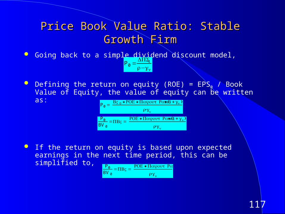
Going back to a simple dividend discount model,

Defining the return on equity (ROE) = EPS0 / Book Value of Equity, the value of equity can be written as:

If the return on equity is based upon expected earnings in the next time period, this can be simplified to,

P 0 =DPS1r−gn

P 0 = BV0 * ROE* Payout Ratio* (1 +gn )

r-gn

P 0

BV 0=PBV =

ROE* Payout Ratio* (1 +gn)

r-gn

P 0

BV 0=PBV =

ROE* Payout Ratio

r-gn

118

Price Book Value Ratio: Stable Growth FirmPrice Book Value Ratio: Stable Growth FirmAnother PresentationAnother Presentation

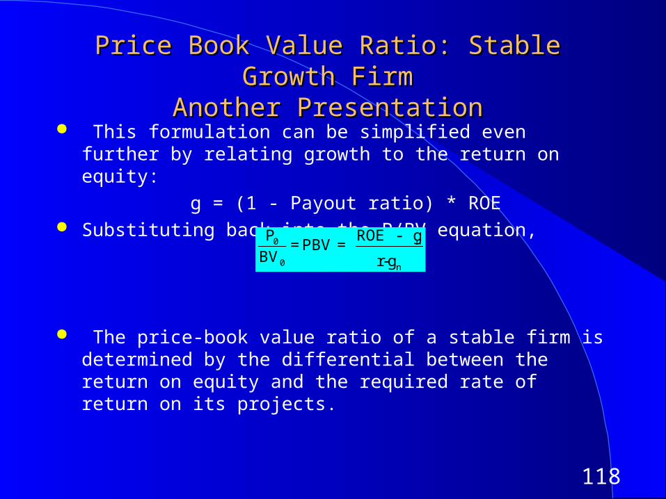
This formulation can be simplified even further by relating growth to the return on equity:

g = (1 - Payout ratio) * ROE Substituting back into the P/BV equation,

The price-book value ratio of a stable firm is determined by the differential between the return on equity and the required rate of return on its projects.

€

P0

BV0

= PBV = ROE - gn

r-gn

119

Price Book Value Ratio for High Growth FirmPrice Book Value Ratio for High Growth Firm

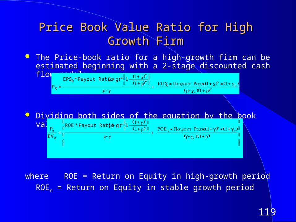
The Price-book ratio for a high-growth firm can be estimated beginning with a 2-stage discounted cash flow model:

Dividing both sides of the equation by the book value of equity:

where ROE = Return on Equity in high-growth period

ROEn = Return on Equity in stable growth period

P 0 =

EPS0 * Payout Ratio * (1 + g) * 1−(1+ g)n

(1+ r)n ⎛

⎝ ⎜ ⎞

⎠ ⎟

r -g+

EPS0 * Payout Ration * (1+g)n * (1+gn)(r-gn)(1+ r)n

P0

BV0

=

ROE* Payout Ratio *(1+ g)* 1−(1+ )g n

(1+ )r n

⎛ ⎝ ⎜ ⎞

⎠

r-g+

ROEn * Payout Ration * (1+ )g n * (1+gn)(r-gn )(1+ )r n

⎡

⎣

⎢ ⎢ ⎢

⎤

⎦

⎥ ⎥ ⎥

120

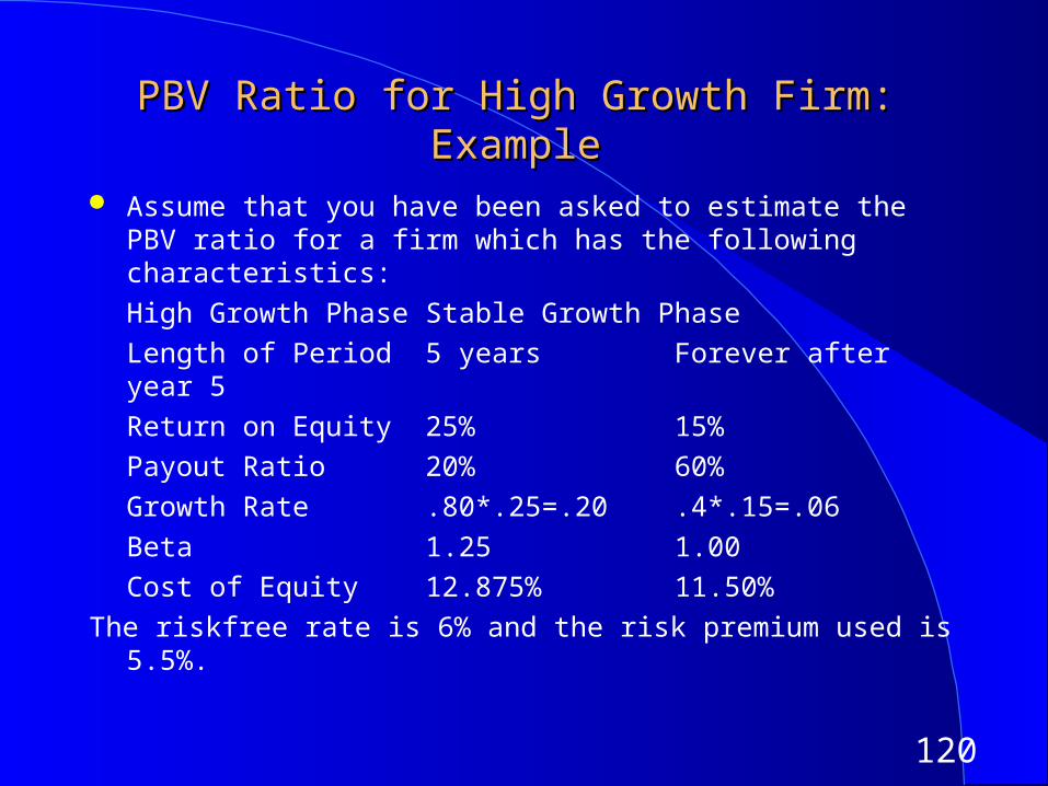
PBV Ratio for High Growth Firm: ExamplePBV Ratio for High Growth Firm: Example

Assume that you have been asked to estimate the PBV ratio for a firm which has the following characteristics:

High Growth Phase Stable Growth Phase

Length of Period 5 years Forever after year 5

Return on Equity 25% 15%

Payout Ratio 20% 60%

Growth Rate .80*.25=.20 .4*.15=.06

Beta 1.25 1.00

Cost of Equity 12.875% 11.50%

The riskfree rate is 6% and the risk premium used is 5.5%.

121

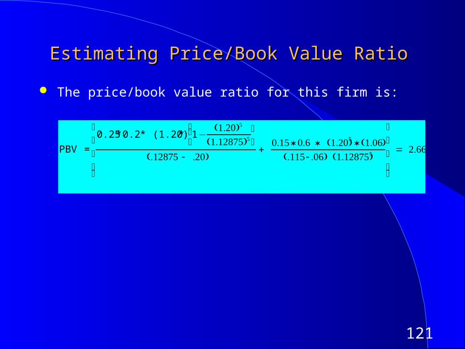
Estimating Price/Book Value RatioEstimating Price/Book Value Ratio

The price/book value ratio for this firm is:

PBV =

0.25 * 0.2 * (1.20) * 1−(1.20)5

(1.12875)5 ⎛ ⎝ ⎜ ⎞

⎠(.12875 - .20)

+ 0.15 * 0.6 * (1.20)5 * (1.06)

(.115 - .06) (1.12875)5

⎡

⎣

⎢ ⎢ ⎢

⎤

⎦

⎥ ⎥ ⎥

= 2.66

122

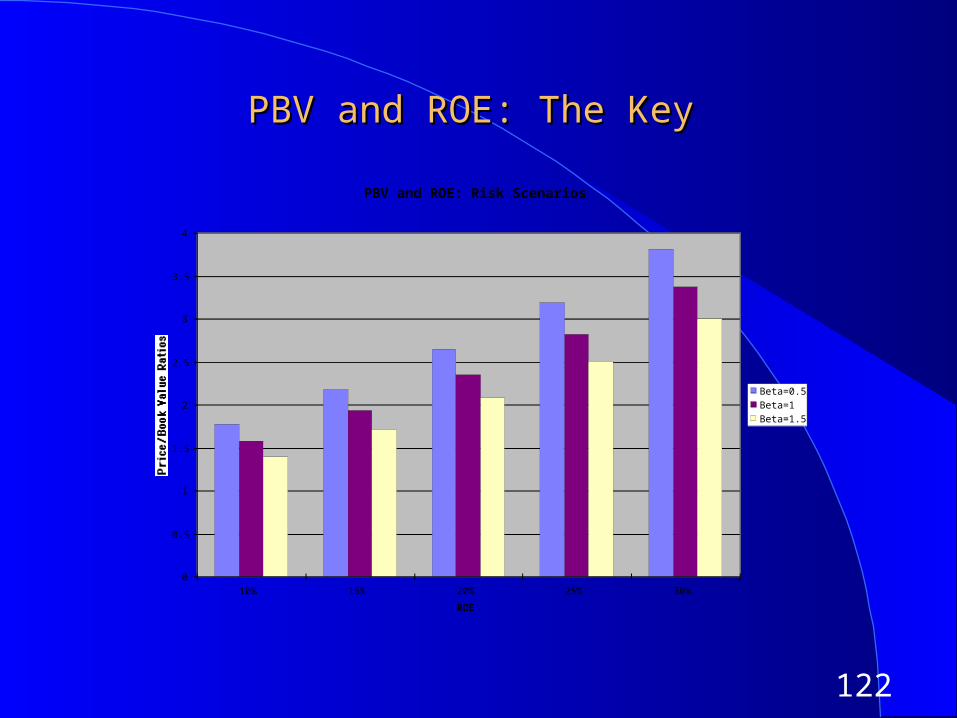
PBV and ROE: The KeyPBV and ROE: The Key

PBV and ROE: Risk Scenarios

0

0.5

1

1.5

2

2.5

3

3.5

4

10% 15% 20% 25% 30%

ROE

Price/Book Value Ratios

Beta=0.5Beta=1Beta=1.5

123

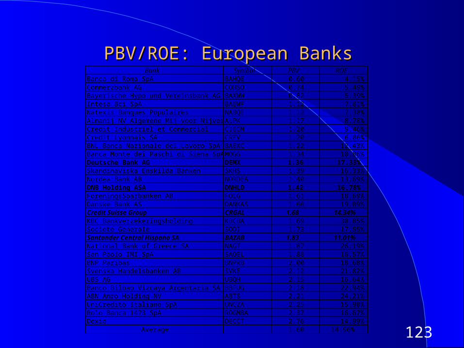
PBV/ROE: European BanksPBV/ROE: European BanksBank Symbol PBV ROE

Banca di Roma SpA BAHQE 0.60 4.15%Commerzbank AG COHSO 0.74 5.49%Bayerische Hypo und Vereinsbank AG BAXWW 0.82 5.39%Intesa Bci SpA BAEWF 1.12 7.81%Natexis Banques Populaires NABQE 1.12 7.38%Almanij NV Algemene Mij voor Nijver ALPK 1.17 8.78%Credit Industriel et Commercial CIECM 1.20 9.46%Credit Lyonnais SA CREV 1.20 6.86%BNL Banca Nazionale del Lavoro SpA BAEXC 1.22 12.43%Banca Monte dei Paschi di Siena SpA MOGG 1.34 10.86%Deutsche Bank AG DEMX 1.36 17.33%Skandinaviska Enskilda Banken SKHS 1.39 16.33%Nordea Bank AB NORDEA 1.40 13.69%DNB Holding ASA DNHLD 1.42 16.78%ForeningsSparbanken AB FOLG 1.61 18.69%Danske Bank AS DANKAS 1.66 19.09%Credit Suisse Group CRGAL 1.68 14.34%KBC Bankverzekeringsholding KBCBA 1.69 30.85%Societe Generale SODI 1.73 17.55%Santander Central Hispano SA BAZAB 1.83 11.01%National Bank of Greece SA NAGT 1.87 26.19%San Paolo IMI SpA SAOEL 1.88 16.57%BNP Paribas BNPRB 2.00 18.68%Svenska Handelsbanken AB SVKE 2.12 21.82%UBS AG UBQH 2.15 16.64%Banco Bilbao Vizcaya Argentaria SA BBFUG 2.18 22.94%ABN Amro Holding NV ABTS 2.21 24.21%UniCredito Italiano SpA UNCZA 2.25 15.90%Rolo Banca 1473 SpA ROGMBA 2.37 16.67%Dexia DECCT 2.76 14.99%

Average 1.60 14.96%

124

PBV versus ROE regressionPBV versus ROE regression

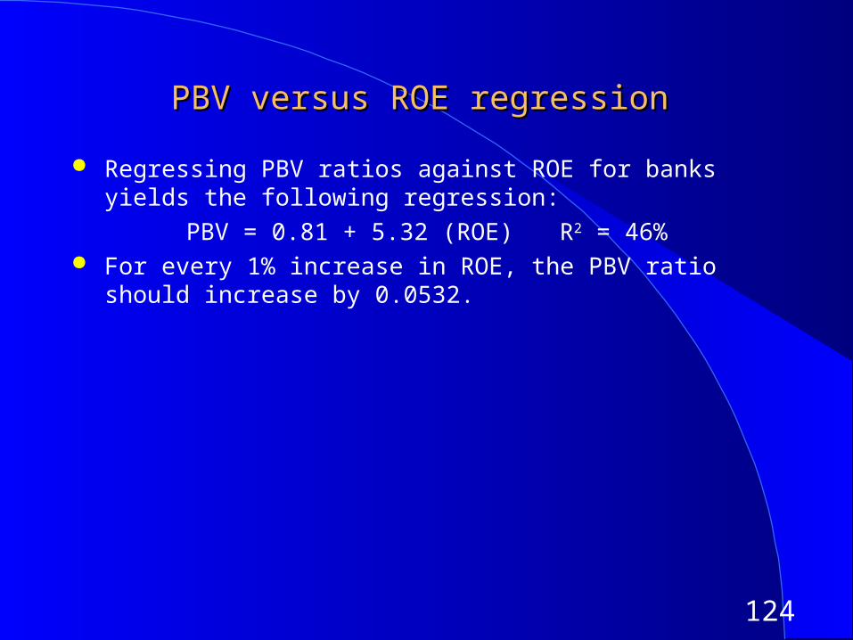
Regressing PBV ratios against ROE for banks yields the following regression:

PBV = 0.81 + 5.32 (ROE) R2 = 46% For every 1% increase in ROE, the PBV ratio should increase by

0.0532.

125

Under and Over Valued Banks?Under and Over Valued Banks?

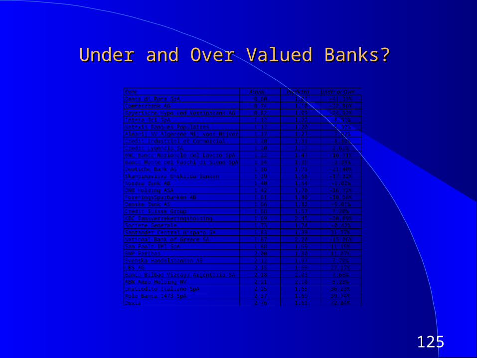
Bank Actual Predicted Under or OverBanca di Roma SpA 0.60 1.03 -41.33%Commerzbank AG 0.74 1.10 -32.86%Bayerische Hypo und Vereinsbank AG 0.82 1.09 -24.92%Intesa Bci SpA 1.12 1.22 -8.51%Natexis Banques Populaires 1.12 1.20 -6.30%Almanij NV Algemene Mij voor Nijver 1.17 1.27 -7.82%Credit Industriel et Commercial 1.20 1.31 -8.30%Credit Lyonnais SA 1.20 1.17 2.61%BNL Banca Nazionale del Lavoro SpA 1.22 1.47 -16.71%Banca Monte dei Paschi di Siena SpA 1.34 1.39 -3.38%Deutsche Bank AG 1.36 1.73 -21.40%Skandinaviska Enskilda Banken 1.39 1.68 -17.32%Nordea Bank AB 1.40 1.54 -9.02%DNB Holding ASA 1.42 1.70 -16.72%ForeningsSparbanken AB 1.61 1.80 -10.66%Danske Bank AS 1.66 1.82 -9.01%Credit Suisse Group 1.68 1.57 7.20%KBC Bankverzekeringsholding 1.69 2.45 -30.89%Societe Generale 1.73 1.74 -0.42%Santander Central Hispano SA 1.83 1.39 31.37%National Bank of Greece SA 1.87 2.20 -15.06%San Paolo IMI SpA 1.88 1.69 11.15%BNP Paribas 2.00 1.80 11.07%Svenska Handelsbanken AB 2.12 1.97 7.70%UBS AG 2.15 1.69 27.17%Banco Bilbao Vizcaya Argentaria SA 2.18 2.03 7.66%ABN Amro Holding NV 2.21 2.10 5.23%UniCredito Italiano SpA 2.25 1.65 36.23%Rolo Banca 1473 SpA 2.37 1.69 39.74%Dexia 2.76 1.61 72.04%

126

Looking for undervalued securities - PBV Looking for undervalued securities - PBV Ratios and ROERatios and ROE

Given the relationship between price-book value ratios and returns on equity, it is not surprising to see firms which have high returns on equity selling for well above book value and firms which have low returns on equity selling at or below book value.

The firms which should draw attention from investors are those which provide mismatches of price-book value ratios and returns on equity - low P/BV ratios and high ROE or high P/BV ratios and low ROE.

127

The Valuation MatrixThe Valuation Matrix

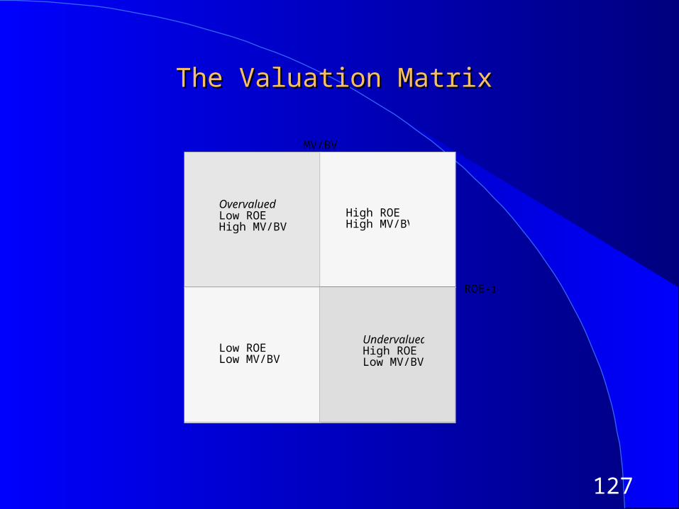
MV/BV

ROE-r

High ROEHigh MV/BV

Low ROELow MV/BV

OvervaluedLow ROEHigh MV/BV

UndervaluedHigh ROELow MV/BV

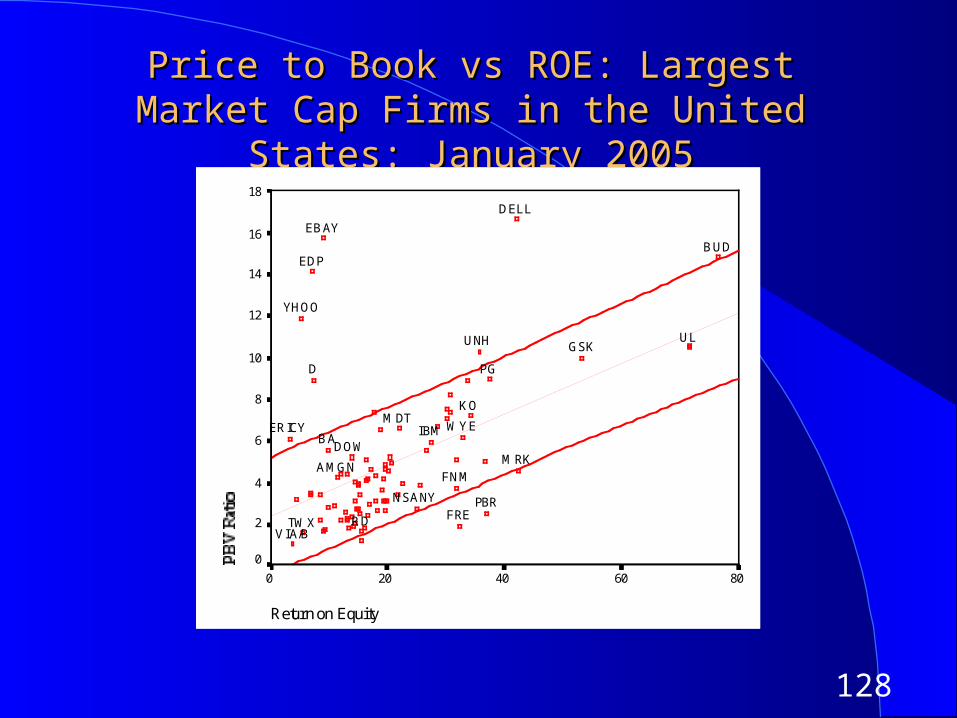
128

Price to Book vs ROE: Largest Market Cap Price to Book vs ROE: Largest Market Cap Firms in the United States: January 2005Firms in the United States: January 2005

Return on Equity

806040200

PBV Ratio

18

16

14

12

10

8

6

4

2

0

BUD

PBR

BADOW

NSANYFRE

ERICY

YHOO

UNH

WYE

D

MDT

VIA/B

UL

FNMMRK

EBAY

AMGN

TWX

EDP

KO

DELL

RD

GSK

PG

IBM

129

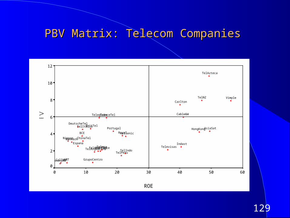
PBV Matrix: Telecom CompaniesPBV Matrix: Telecom Companies

TelAzteca

TelNZ VimpleCarlton

Cable&WTeleglobeFranceTel

DeutscheTelBritTelTelItalia

AsiaSatPortugal HongKongRoyalBCE Hellenic

ChinaTelNipponDanmarkEspana Indast

TelevisasTelmexTelArgFrancePhilTelTelArgentina TelIndoTelPeru

GrupoCentroAPTCallNetAnonima

ROE

6050403020100

12

10

8

6

4

2

0

130

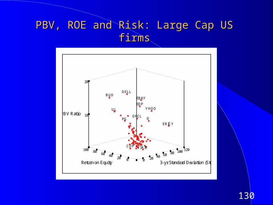
PBV, ROE and Risk: Large Cap US firmsPBV, ROE and Risk: Large Cap US firms

120100

PBV Ratio

ERICY

100

UL

80

10

BUD

ORCL

8060

20

60

D

3-yr Standard Deviation (Stock Price)Return on Equity

PG

YHOO

DELL

VIA/B

40 40

COP

20 20

EBAY

EDP

0 0

131

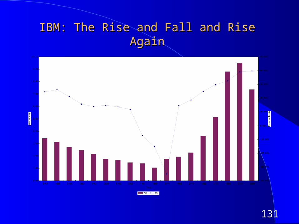
IBM: The Rise and Fall and Rise AgainIBM: The Rise and Fall and Rise Again

0.00

1.00

2.00

3.00

4.00

5.00

6.00

7.00

8.00

9.00

10.00

1983 1984 1985 1986 1987 1988 1989 1990 1991 1992 1993 1994 1995 1996 1997 1998 1999 2000

Year

Price to Book

-40.00%

-30.00%

-20.00%

-10.00%

0.00%

10.00%

20.00%

30.00%

40.00%

50.00%

Return on Equity

PBV ROE

132

PBV Ratio Regression: USPBV Ratio Regression: USJanuary 2005January 2005

133

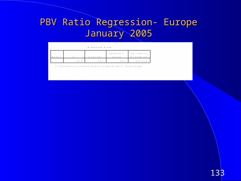
PBV Ratio Regression- EuropePBV Ratio Regression- EuropeJanuary 2005January 2005

M o d e l S u m m a r y

. 4 9 6a

. 2 4 6 . 2 4 5 1 9 7 . 9 1 6

M o d e l

1

R R S q u a r e

A d j u s t e d R

S q u a r e

S t d . E r r o r o f

t h e E s t i m a t e

P r e d i c t o r s : ( C o n s t a n t ) , R e t u r n o n E q u i t y , B E T A , P a y o u t R a t i oa .

134

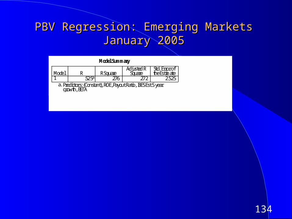
PBV Regression: Emerging MarketsPBV Regression: Emerging MarketsJanuary 2005January 2005

Model Summary

.525a .276 .272 2.525Model1

R R SquareAdjusted R

SquareStd. Error ofthe Estimate

Predictors: (Constant), ROE, Payout Ratio, IBES Est 5 yeargrowth, BETA

a.

135

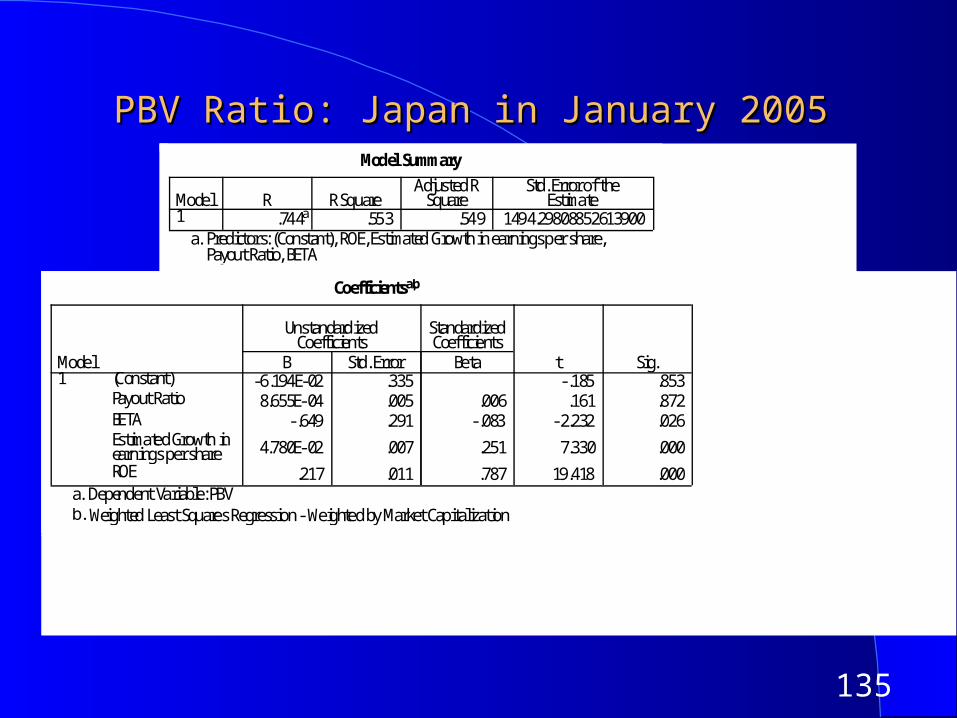
PBV Ratio: Japan in January 2005PBV Ratio: Japan in January 2005Model Summary

.744a .553 .549 1494.29808852613900Model1

R R SquareAdjusted R

SquareStd. Error of the

Estimate

Predictors: (Constant), ROE, Estimated Growth in earnings per share,Payout Ratio, BETA

a.

Coefficientsa,b

-6.194E-02 .335 -.185 .8538.655E-04 .005 .006 .161 .872

-.649 .291 -.083 -2.232 .026

4.780E-02 .007 .251 7.330 .000

.217 .011 .787 19.418 .000

(Constant)Payout RatioBETAEstimated Growth inearnings per shareROE

Model1

B Std. Error

UnstandardizedCoefficients

Beta

StandardizedCoefficients

t Sig.

Dependent Variable: PBVa. Weighted Least Squares Regression - Weighted by Market Capitalizationb.

136

Value/Book Value Ratio: DefinitionValue/Book Value Ratio: Definition

While the price to book ratio is a equity multiple, both the market value and the book value can be stated in terms of the firm.

Value/Book Value = Market Value of Equity + Market Value of Debt

Book Value of Equity + Book Value of Debt

137

Determinants of Value/Book RatiosDeterminants of Value/Book Ratios

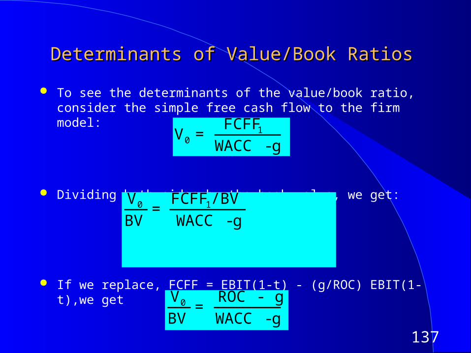
To see the determinants of the value/book ratio, consider the simple free cash flow to the firm model:

Dividing both sides by the book value, we get:

If we replace, FCFF = EBIT(1-t) - (g/ROC) EBIT(1-t),we get

V0 = FCFF1

WACC - g

V0

BV=

FCFF1/BV

WACC - g

V0

BV=

ROC - g

WACC - g

138

Value/Book Ratio: An ExampleValue/Book Ratio: An Example

Consider a stable growth firm with the following characteristics:– Return on Capital = 12%

– Cost of Capital = 10%

– Expected Growth = 5% The value/BV ratio for this firm can be estimated as follows:

Value/BV = (.12 - .05)/(.10 - .05) = 1.40 The effects of ROC on growth will increase if the firm has a high

growth phase, but the basic determinants will remain unchanged.

139

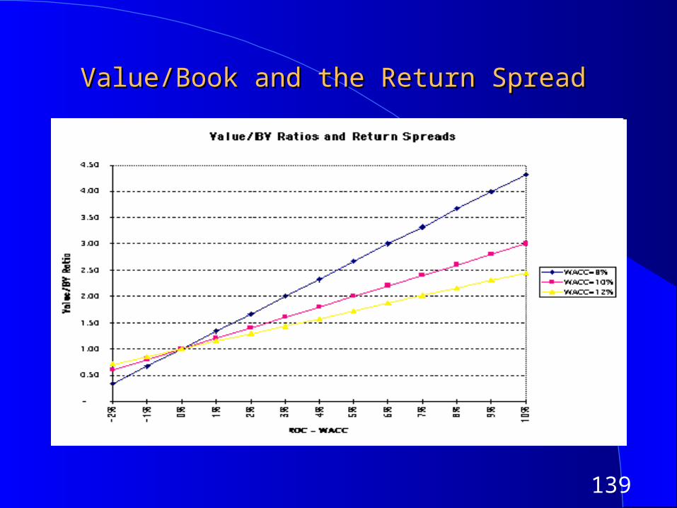
Value/Book and the Return SpreadValue/Book and the Return Spread

140

Value/Book Capital Regression - US - January Value/Book Capital Regression - US - January 20052005

M o d e l S u m m a r y

. 7 0 8a

. 5 0 1 . 4 9 9 1 5 9 . 3 4 8 3 4 3 5 5 3 4 4 4 8 0 0

M o d e l

1

R R S q u a r e

A d j u s t e d R

S q u a r e S t d . E r r o r o f t h e E s t i m a t e

P r e d i c t o r s : ( C o n s t a n t ), R e t u r n o n C a p i t a l , E x p e c t e d G r o w t h i n R e v e n u e s : n e x t 5 y e a r s ,

R e i n v e s t m e n t R a t e , M a r k e t D e b t t o C a p i ta l

a .

141

Price Sales Ratio: DefinitionPrice Sales Ratio: Definition

The price/sales ratio is the ratio of the market value of equity to the sales.

Price/ Sales= Market Value of Equity

Total Revenues Consistency Tests

– The price/sales ratio is internally inconsistent, since the market value of equity is divided by the total revenues of the firm.

142

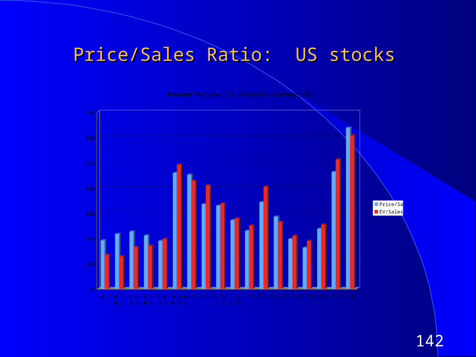
Price/Sales Ratio: US stocksPrice/Sales Ratio: US stocks

0

100

200

300

400

500

600

700

<0.1 0.1-0.2

0.2-0.3

0.3-0.4

0.4-0.5

0.5-0.75

0.75-1 1-1.25 1.25-1.5

1.5-1.75

1.75-2 2-2.5 2.5-3 3-3.5 3.5-4 4-5 5-10 >10

Revenue Multiples: US companies in January 2005

Price/Sales

EV/Sales

143

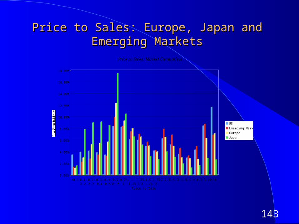
Price to Sales: Europe, Japan and Emerging Price to Sales: Europe, Japan and Emerging MarketsMarkets

0.00%

2.00%

4.00%

6.00%

8.00%

10.00%

12.00%

14.00%

16.00%

18.00%

% of Firms in Market

<0.1 0.1-0.2

0.2-0.3

0.3-0.4

0.4-0.5

0.5-0.75

0.75-1

1-1.25

1.25-1.5

1.5-1.75

1.75-2

2-2.5 2.5-3 3-3.5 3.5-4 4-5 5-10 >10

Price to Sales Ratio

Price to Sales: Market Comparisons

US

Emerging Markets

Europe

Japan

144

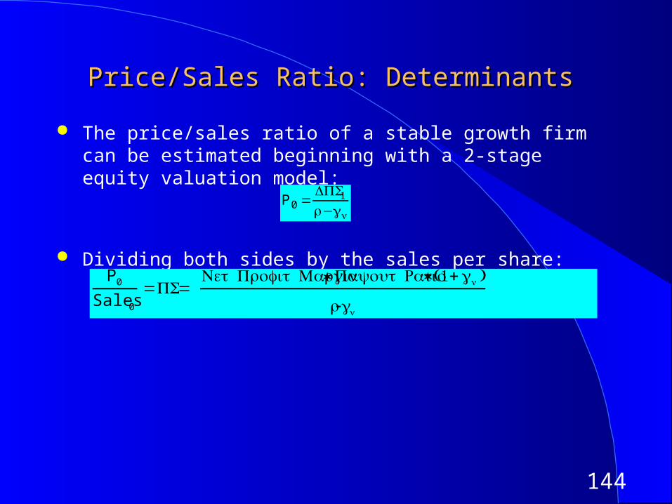
Price/Sales Ratio: DeterminantsPrice/Sales Ratio: Determinants

The price/sales ratio of a stable growth firm can be estimated beginning with a 2-stage equity valuation model:

Dividing both sides by the sales per share:

P 0 =DPS1r−gn

P0

Sales0

=PS= Net Profit Margin* Payout Ratio* (1+gn )

r-gn

145

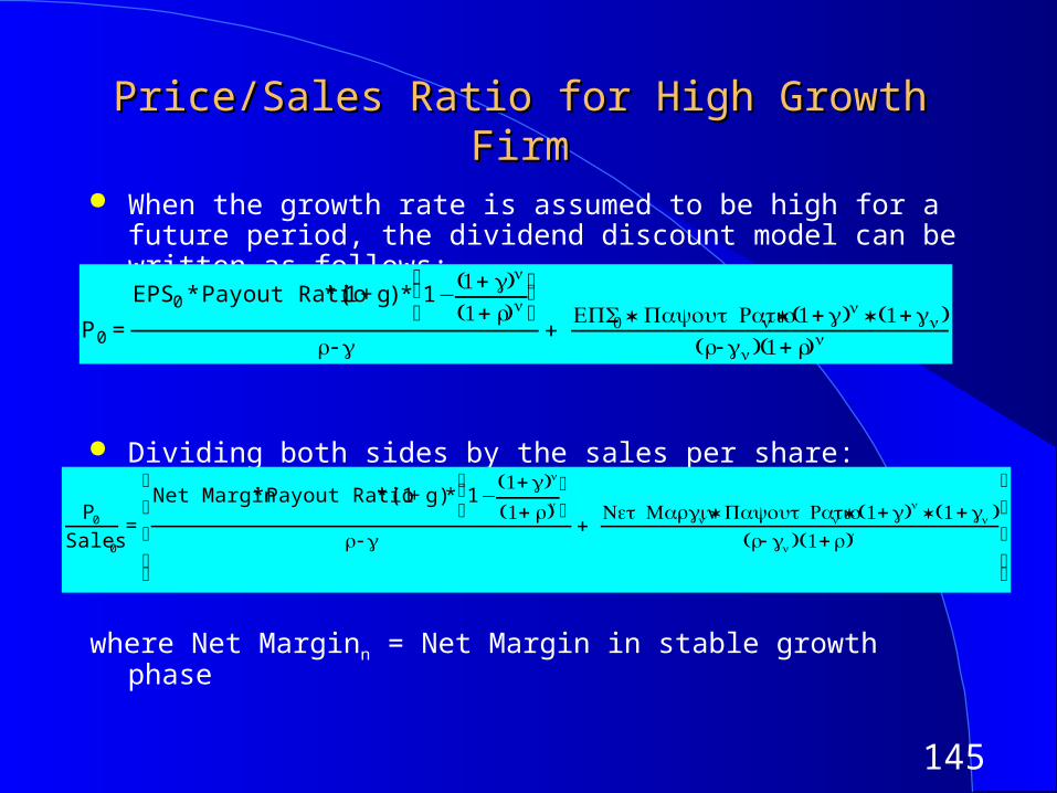
Price/Sales Ratio for High Growth FirmPrice/Sales Ratio for High Growth Firm

When the growth rate is assumed to be high for a future period, the dividend discount model can be written as follows:

Dividing both sides by the sales per share:

where Net Marginn = Net Margin in stable growth phase

P 0 =

EPS0 * Payout Ratio * (1 + g) * 1−(1+ g)n

(1+ r)n ⎛

⎝ ⎜ ⎞

⎠ ⎟

r -g+

EPS0 * Payout Ration * (1+g)n * (1+gn)(r-gn)(1+ r)n

P0

Sales0

=

Net Margin * Payout Ratio * (1+ g)* 1−(1+ )g n

(1+ )r n

⎛ ⎝ ⎜ ⎞

⎠r -g

+ Net Marginn * Payout Ration * (1+ )g n * (1 +gn )

(r- gn)(1 + )r n

⎡

⎣

⎢ ⎢ ⎢

⎤

⎦

⎥ ⎥ ⎥

146

Price Sales Ratios and Profit MarginsPrice Sales Ratios and Profit Margins

The key determinant of price-sales ratios is the profit margin. A decline in profit margins has a two-fold effect.

– First, the reduction in profit margins reduces the price-sales ratio directly.

– Second, the lower profit margin can lead to lower growth and hence lower price-sales ratios.

Expected growth rate = Retention ratio * Return on Equity

= Retention Ratio *(Net Profit / Sales) * ( Sales / BV of Equity)

= Retention Ratio * Profit Margin * Sales/BV of Equity

147

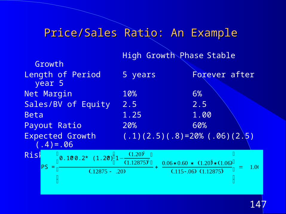
Price/Sales Ratio: An ExamplePrice/Sales Ratio: An Example

High Growth Phase Stable GrowthLength of Period 5 years Forever after year 5Net Margin 10% 6%Sales/BV of Equity 2.5 2.5Beta 1.25 1.00Payout Ratio 20% 60%Expected Growth (.1)(2.5)(.8)=20% (.06)(2.5)(.4)=.06Riskless Rate =6%

PS =

0.10 * 0.2 * (1.20) * 1−(1.20)5

(1.12875)5 ⎛ ⎝ ⎜ ⎞

⎠(.12875 - .20)

+ 0.06 * 0.60 * (1.20)5 * (1.06)

(.115 -.06) (1.12875)5

⎡

⎣

⎢ ⎢ ⎢

⎤

⎦

⎥ ⎥ ⎥

= 1.06

148

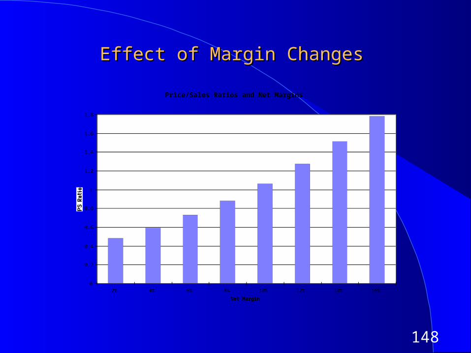
Effect of Margin ChangesEffect of Margin Changes

Price/Sales Ratios and Net Margins

0

0.2

0.4

0.6

0.8

1

1.2

1.4

1.6

1.8

2% 4% 6% 8% 10% 12% 14% 16%

Net Margin

PS Ratio

149

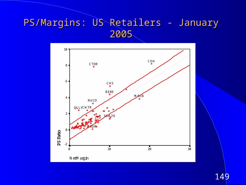
PS/Margins: US Retailers - January 2005PS/Margins: US Retailers - January 2005

Net Margin

3020100

PS Ratio

10

8

6

4

2

0

-2

SGB.TO

QGLY

NUCOMRLN

LTD

FRDM

CWTR

COH

CHS

CTHR

BEBE

150

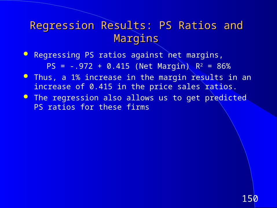
Regression Results: PS Ratios and MarginsRegression Results: PS Ratios and Margins

Regressing PS ratios against net margins,

PS = -.972 + 0.415 (Net Margin) R2 = 86% Thus, a 1% increase in the margin results in an increase of 0.415 in the

price sales ratios. The regression also allows us to get predicted PS ratios for these firms

151

Current versus Predicted MarginsCurrent versus Predicted Margins

One of the limitations of the analysis we did in these last few pages is the focus on current margins. Stocks are priced based upon expected margins rather than current margins.

For most firms, current margins and predicted margins are highly correlated, making the analysis still relevant.

For firms where current margins have little or no correlation with expected margins, regressions of price to sales ratios against current margins (or price to book against current return on equity) will not provide much explanatory power.

In these cases, it makes more sense to run the regression using either predicted margins or some proxy for predicted margins.

152

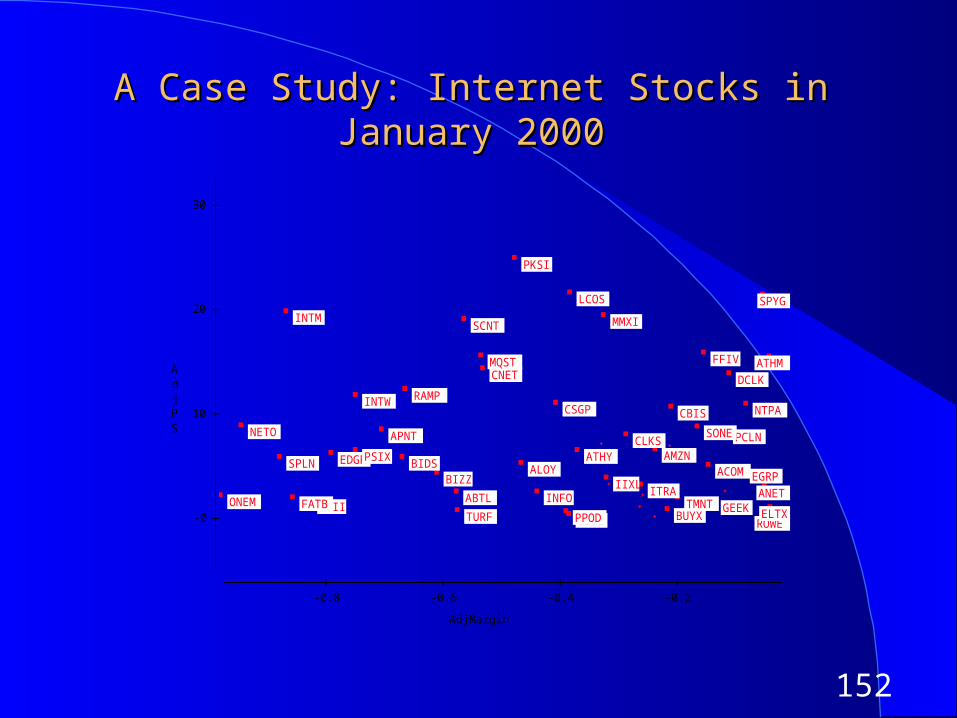
A Case Study: Internet Stocks in January 2000A Case Study: Internet Stocks in January 2000

ROWEGSVIPPODTURF BUYX ELTXGEEKRMIIFATB TMNTONEM ABTL INFO ANETITRAIIXLBIZZ EGRPACOMALOYBIDSSPLN EDGRPSIX ATHY AMZN

CLKS PCLNAPNT SONENETO

CBIS NTPACSGPINTW RAMP

DCLKCNETATHMMQST FFIV

SCNT MMXIINTMSPYGLCOS

PKSI

-0

10

20

30

-0.8 -0.6 -0.4 -0.2

AdjMargin

AdjPS

153

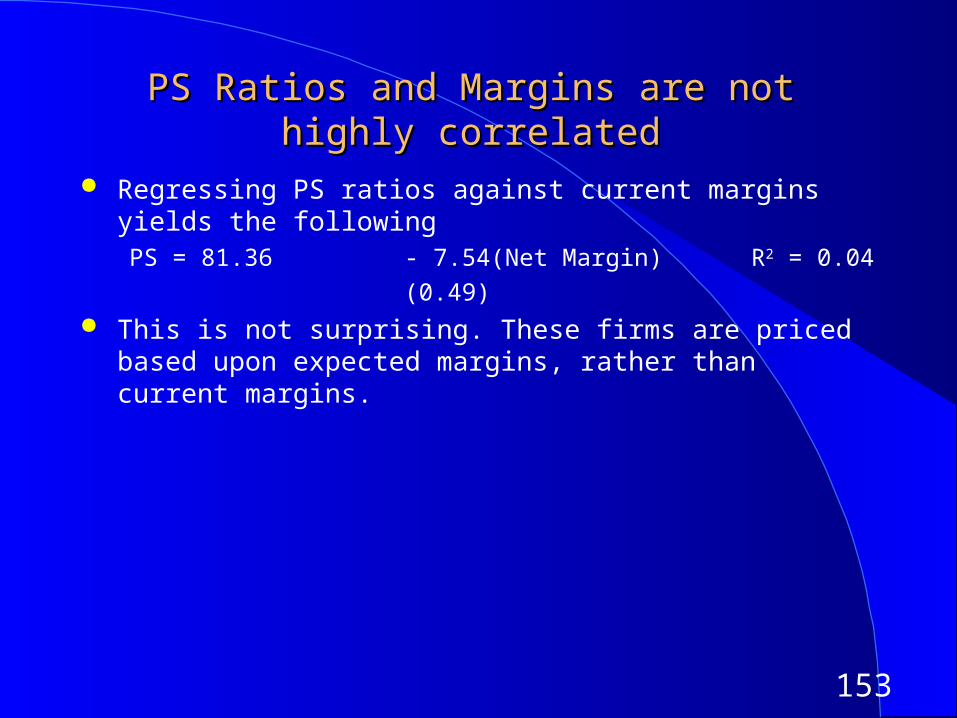
PS Ratios and Margins are not highly PS Ratios and Margins are not highly correlatedcorrelated

Regressing PS ratios against current margins yields the followingPS = 81.36 - 7.54(Net Margin) R2 = 0.04

(0.49) This is not surprising. These firms are priced based upon expected

margins, rather than current margins.

154

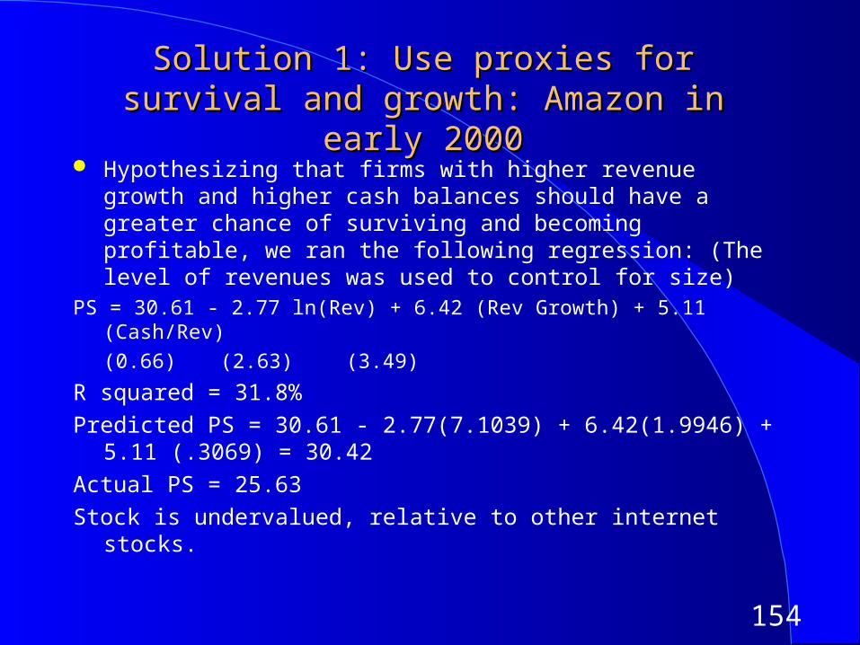
Solution 1: Use proxies for survival and Solution 1: Use proxies for survival and growth: Amazon in early 2000growth: Amazon in early 2000

Hypothesizing that firms with higher revenue growth and higher cash balances should have a greater chance of surviving and becoming profitable, we ran the following regression: (The level of revenues was used to control for size)

PS = 30.61 - 2.77 ln(Rev) + 6.42 (Rev Growth) + 5.11 (Cash/Rev)

(0.66) (2.63) (3.49)

R squared = 31.8%

Predicted PS = 30.61 - 2.77(7.1039) + 6.42(1.9946) + 5.11 (.3069) = 30.42

Actual PS = 25.63

Stock is undervalued, relative to other internet stocks.

155

Solution 2: Use forward multiplesSolution 2: Use forward multiples

You can always estimate price (or value) as a multiple of revenues, earnings or book value in a future year. These multiples are called forward multiples.

For young and evolving firms, the values of fundamentals in future years may provide a much better picture of the true value potential of the firm. There are two ways in which you can use forward multiples:– Look at value today as a multiple of revenues or earnings in the future

(say 5 years from now) for all firms in the comparable firm list. Use the average of this multiple in conjunction with your firm’s earnings or revenues to estimate the value of your firm today.

– Estimate value as a multiple of current revenues or earnings for more mature firms in the group and apply this multiple to the forward earnings or revenues to the forward earnings for your firm. This will yield the expected value for your firm in the forward year and will have to be discounted back to the present to get current value.

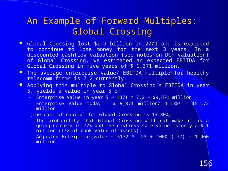
156

An Example of Forward Multiples: Global An Example of Forward Multiples: Global CrossingCrossing

Global Crossing lost $1.9 billion in 2001 and is expected to continue to lose money for the next 3 years. In a discounted cashflow valuation (see notes on DCF valuation) of Global Crossing, we estimated an expected EBITDA for Global Crossing in five years of $ 1,371 million.

The average enterprise value/ EBITDA multiple for healthy telecomm firms is 7.2 currently.

Applying this multiple to Global Crossing’s EBITDA in year 5, yields a value in year 5 of

– Enterprise Value in year 5 = 1371 * 7.2 = $9,871 million– Enterprise Value today = $ 9,871 million/ 1.1385 = $5,172 million(The cost of capital for Global Crossing is 13.80%)– The probability that Global Crossing will not make it as a going concern is 77% and

the distress sale value is only a $ 1 billion (1/2 of book value of assets).– Adjusted Enterprise value = 5172 * .23 + 1000 (.77) = 1,960 million

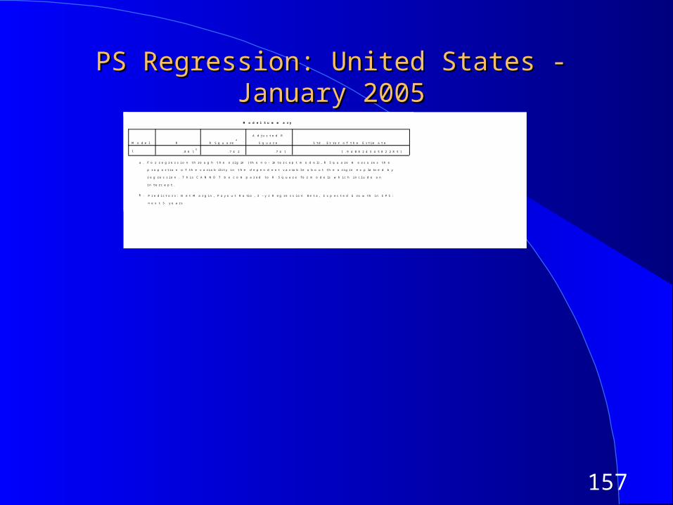
157

PS Regression: United States - January 2005PS Regression: United States - January 2005

M o d e l S u m m a r y

. 8 6 1b

. 7 4 2 . 7 4 1 1 . 9 4 0 8 2 4 3 4 5 8 2 2 8 5 1

M o d e l

1

R R S q u a r ea

A d j u s t e d R

S q u a r e S t d . E r r o r o f t h e E s t i m a t e

F o r r e g r e s s i o n t h r o u g h t h e o r i g i n ( t h e n o - i n t e r c e p t m o d e l ) , R S q u a r e m e a s u r e s t h e

p r o p o r t i o n o f t h e v a r i a b i l i t y i n t h e d e p e n d e n t v a r i a b l e a b o u t t h e o r i g i n e x p l a i n e d b y

r e g r e s s i o n . T h i s C A N N O T b e c o m p a r e d t o R S q u a r e f o r m o d e l s w h i c h i n c l u d e a n

i n t e r c e p t .

a .

P r e d i c t o r s : N e t M a r g i n , P a y o u t R a ti o , 3 - y r R e g r e s s i o n B e t a , E x p e c t e d G r o w t h i n E P S :

n e x t 5 y e a r s

b .

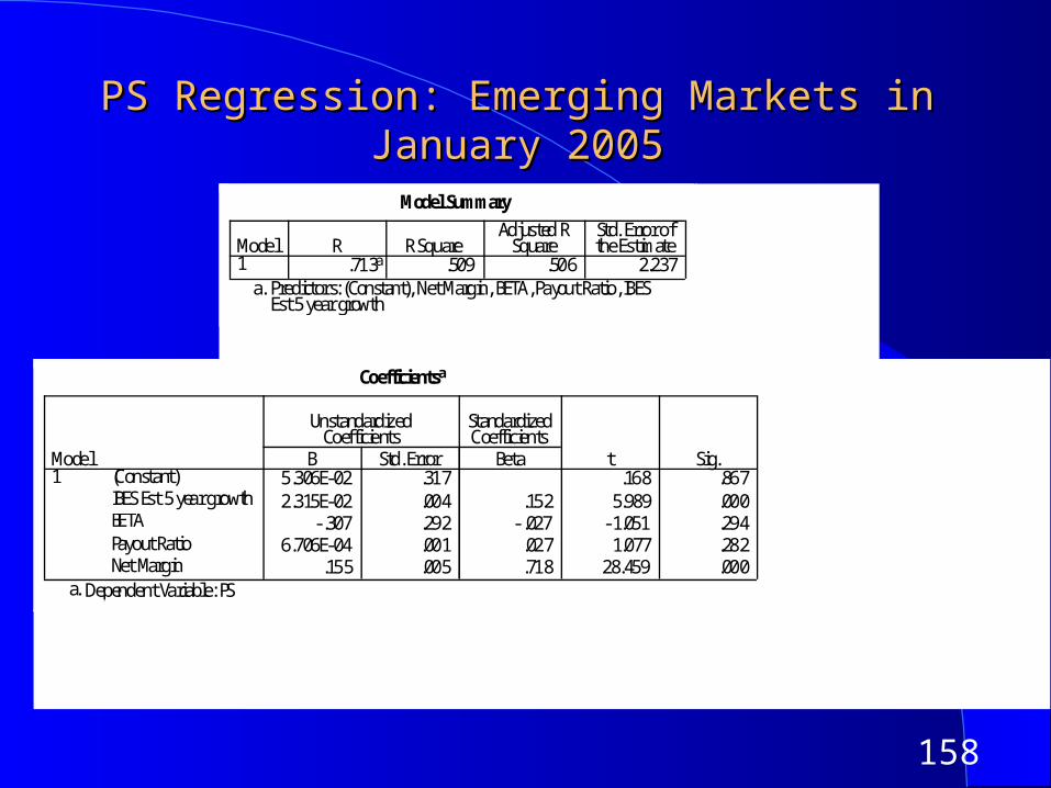
158

PS Regression: Emerging Markets in January PS Regression: Emerging Markets in January 20052005

Model Summary

.713a .509 .506 2.237Model1

R R SquareAdjusted R

SquareStd. Error ofthe Estimate

Predictors: (Constant), Net Margin, BETA, Payout Ratio, IBESEst 5 year growth

a.

Coefficientsa

5.306E-02 .317 .168 .8672.315E-02 .004 .152 5.989 .000

-.307 .292 -.027 -1.051 .2946.706E-04 .001 .027 1.077 .282

.155 .005 .718 28.459 .000

(Constant)IBES Est 5 year growthBETAPayout RatioNet Margin

Model1

B Std. Error

UnstandardizedCoefficients

Beta

StandardizedCoefficients

t Sig.

Dependent Variable: PSa.

159

Value/Sales Ratio: DefinitionValue/Sales Ratio: Definition

The value/sales ratio is the ratio of the market value of the firm to the sales.

Value/ Sales= Market Value of Equity + Market Value of Debt-Cash

Total Revenues

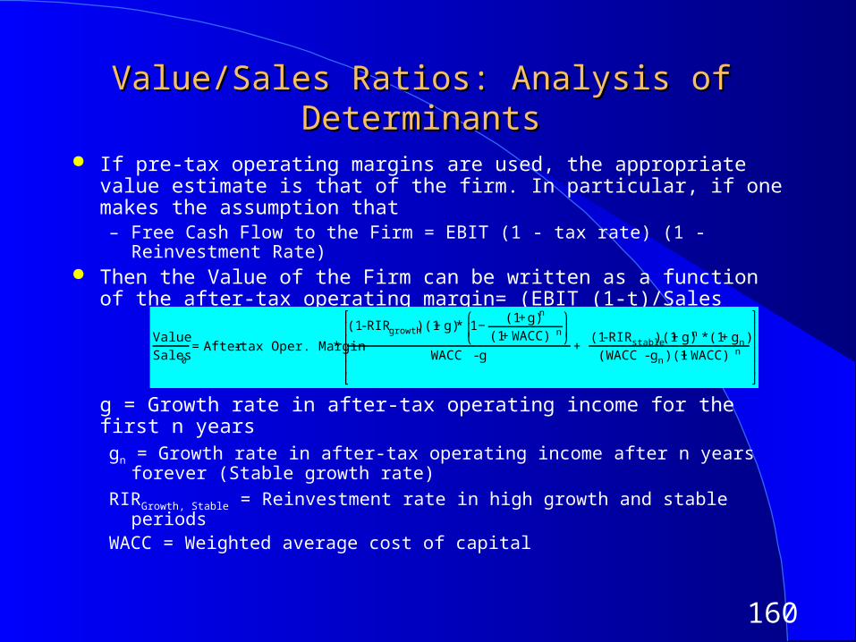
160

Value/Sales Ratios: Analysis of DeterminantsValue/Sales Ratios: Analysis of Determinants

If pre-tax operating margins are used, the appropriate value estimate is that of the firm. In particular, if one makes the assumption that– Free Cash Flow to the Firm = EBIT (1 - tax rate) (1 - Reinvestment Rate)

Then the Value of the Firm can be written as a function of the after-tax operating margin= (EBIT (1-t)/Sales

g = Growth rate in after-tax operating income for the first n yearsgn = Growth rate in after-tax operating income after n years forever (Stable

growth rate)

RIRGrowth, Stable = Reinvestment rate in high growth and stable periodsWACC = Weighted average cost of capital

Value Sales0

=After- tax Oper. Margin*

(1-RIRgrowth)(1+g)* 1−(1+g)n

(1+WACC)n

⎛

⎝ ⎜

⎞

⎠ ⎟

WACC -g+

(1-RIR stable)(1+g)n *(1+gn)(WACC-gn)(1+WACC)n

⎡

⎣

⎢ ⎢ ⎢ ⎢

⎤

⎦

⎥ ⎥ ⎥ ⎥

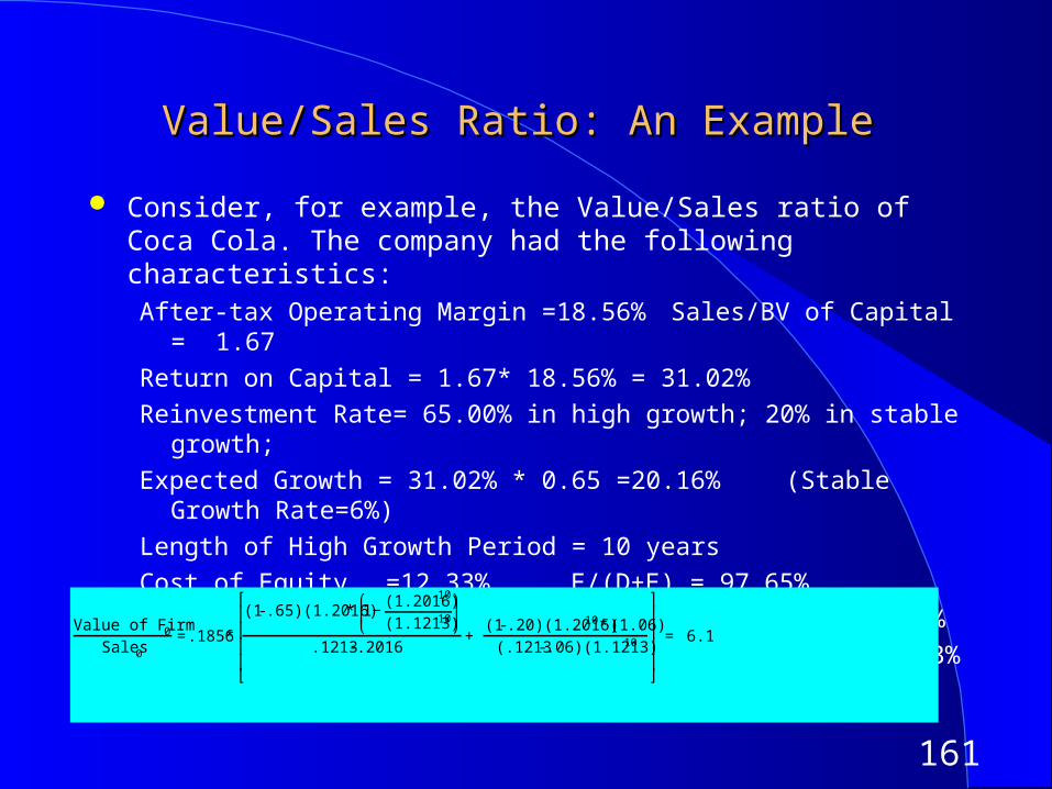
161

Value/Sales Ratio: An ExampleValue/Sales Ratio: An Example

Consider, for example, the Value/Sales ratio of Coca Cola. The company had the following characteristics:After-tax Operating Margin =18.56% Sales/BV of Capital = 1.67

Return on Capital = 1.67* 18.56% = 31.02%

Reinvestment Rate= 65.00% in high growth; 20% in stable growth;

Expected Growth = 31.02% * 0.65 =20.16% (Stable Growth Rate=6%)

Length of High Growth Period = 10 years

Cost of Equity =12.33% E/(D+E) = 97.65%

After-tax Cost of Debt = 4.16% D/(D+E) 2.35%

Cost of Capital= 12.33% (.9765)+4.16% (.0235) = 12.13%

Value of Firm0Sales0

=.1856*

(1- .65)(1.2016)* 1−(1.2016)10

(1.1213)10

⎛

⎝ ⎜

⎞

⎠ ⎟

.1213- .2016+

(1- .20)(1.2016)10* (1.06)(.1213- .06)(1.1213)10

⎡

⎣

⎢ ⎢ ⎢ ⎢

⎤

⎦

⎥ ⎥ ⎥ ⎥

= 6.10

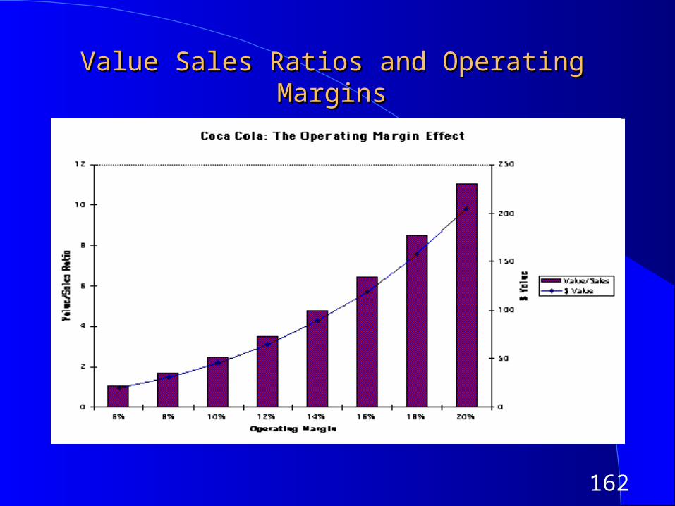
162

Value Sales Ratios and Operating MarginsValue Sales Ratios and Operating Margins

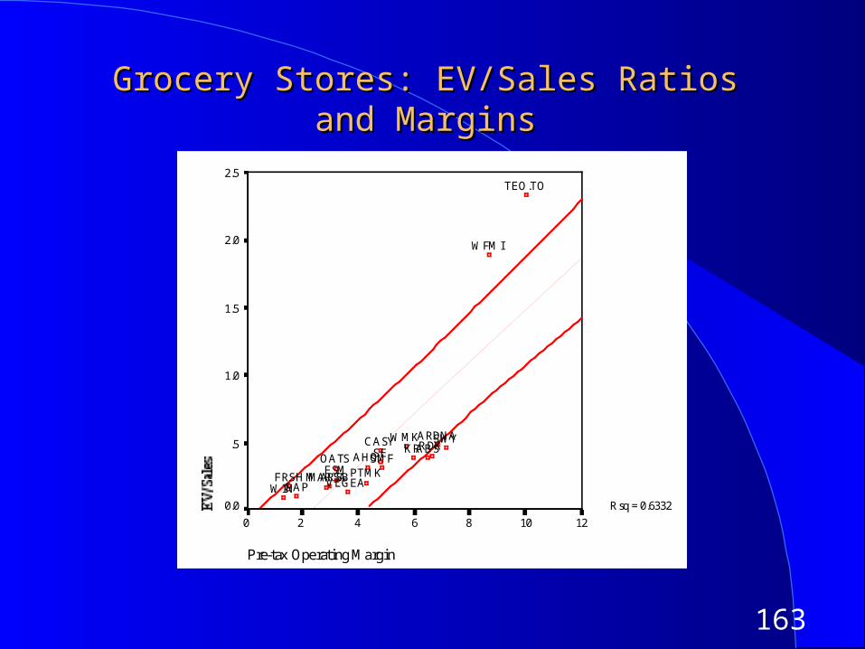
163

Grocery Stores: EV/Sales Ratios and MarginsGrocery Stores: EV/Sales Ratios and Margins

Pre-tax Operating Margin

121086420

EV/Sales

2.5

2.0

1.5

1.0

.5

0.0 Rsq = 0.6332

WIN

OATS

WFMI

WMK

VLGEA

TEO.TO

SMF

SWYRDK

PTMKMARSBMARSA

KR

GAPFRSH

FSM

CASY ARDNAABS

AHOSE

164

Brand Name Premiums in ValuationBrand Name Premiums in Valuation

You have been hired to value Coca Cola for an analyst reports and you have valued the firm at 6.10 times revenues, using the model described in the last few pages. Another analyst is arguing that there should be a premium added on to reflect the value of the brand name. Do you agree?

Yes No Explain.

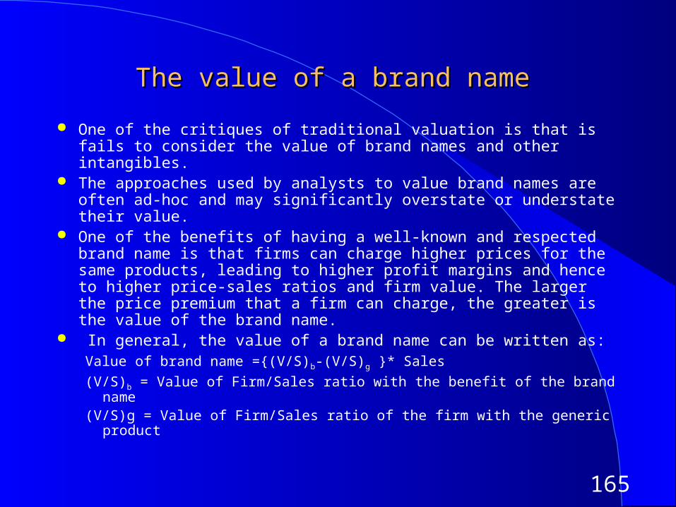
165

The value of a brand nameThe value of a brand name

One of the critiques of traditional valuation is that is fails to consider the value of brand names and other intangibles.

The approaches used by analysts to value brand names are often ad-hoc and may significantly overstate or understate their value.

One of the benefits of having a well-known and respected brand name is that firms can charge higher prices for the same products, leading to higher profit margins and hence to higher price-sales ratios and firm value. The larger the price premium that a firm can charge, the greater is the value of the brand name.

In general, the value of a brand name can be written as:Value of brand name ={(V/S)b-(V/S)g }* Sales

(V/S)b = Value of Firm/Sales ratio with the benefit of the brand name(V/S)g = Value of Firm/Sales ratio of the firm with the generic product

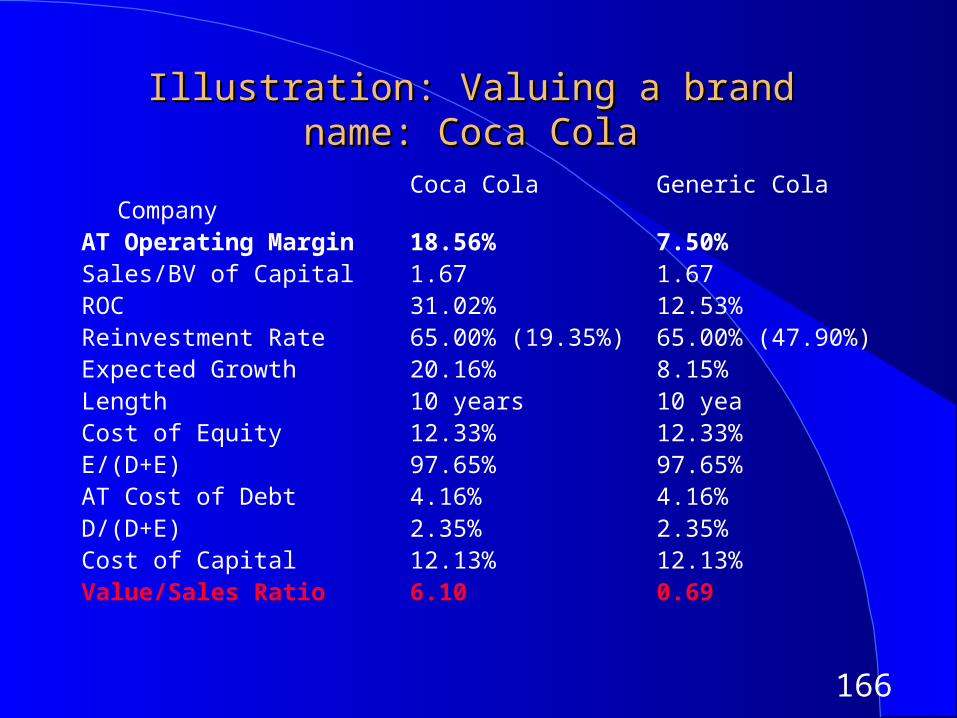
166

Illustration: Valuing a brand name: Coca ColaIllustration: Valuing a brand name: Coca Cola

Coca Cola Generic Cola Company

AT Operating Margin 18.56% 7.50%Sales/BV of Capital 1.67 1.67ROC 31.02% 12.53%Reinvestment Rate 65.00% (19.35%) 65.00% (47.90%)Expected Growth 20.16% 8.15%Length 10 years 10 yeaCost of Equity 12.33% 12.33%E/(D+E) 97.65% 97.65%AT Cost of Debt 4.16% 4.16%D/(D+E) 2.35% 2.35%Cost of Capital 12.13% 12.13%Value/Sales Ratio 6.10 0.69

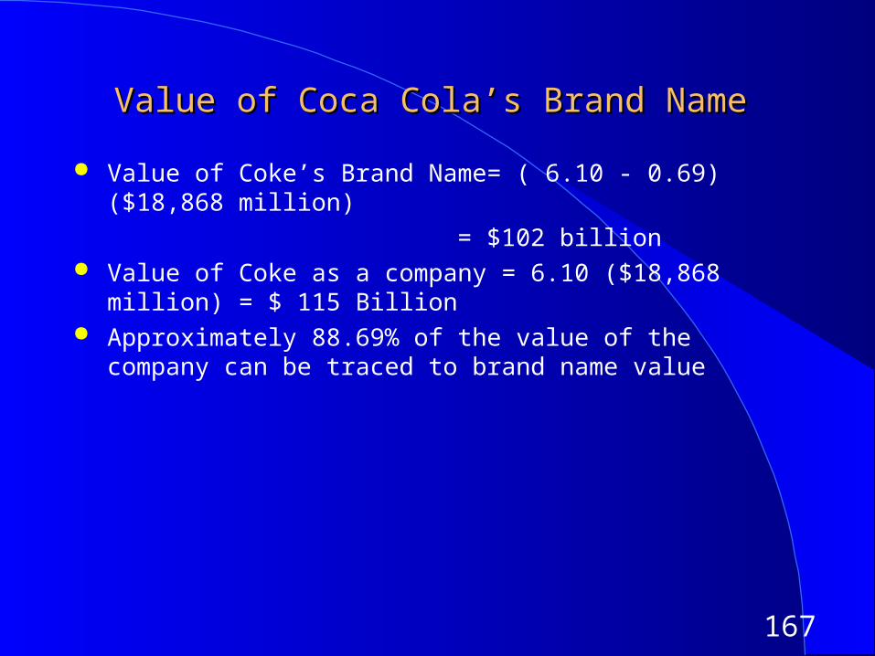
167

Value of Coca Cola’s Brand NameValue of Coca Cola’s Brand Name

Value of Coke’s Brand Name= ( 6.10 - 0.69) ($18,868 million)

= $102 billion Value of Coke as a company = 6.10 ($18,868 million) = $ 115 Billion Approximately 88.69% of the value of the company can be traced to

brand name value

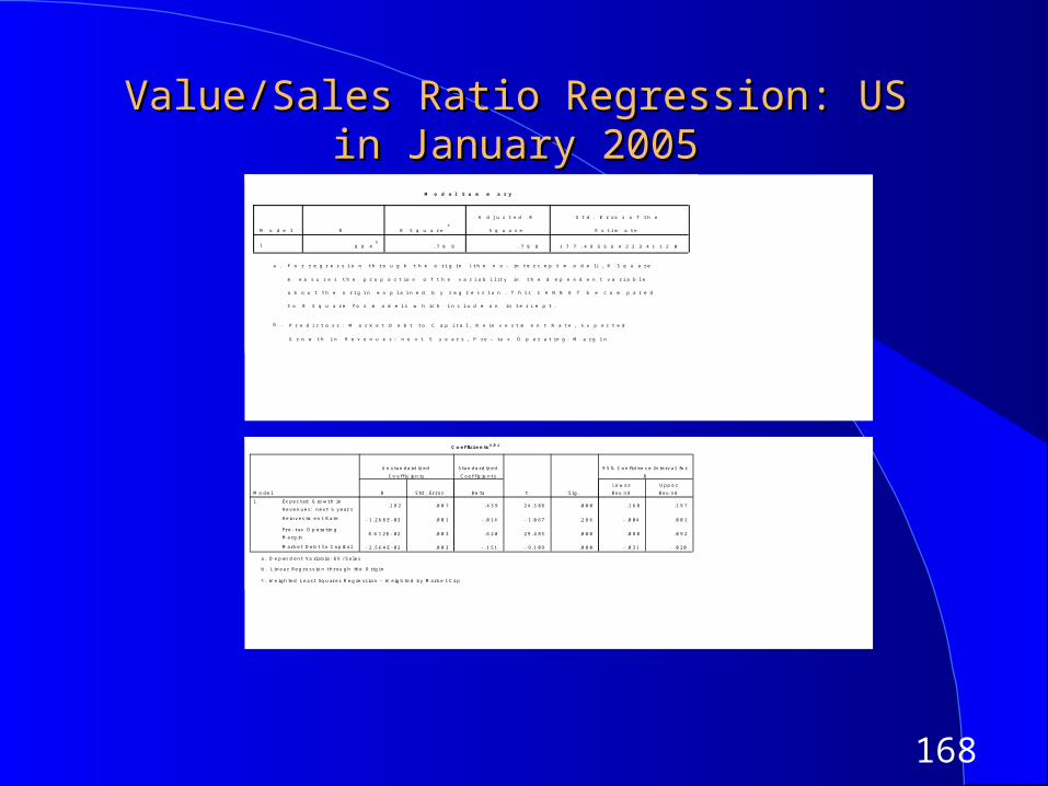
168

Value/Sales Ratio Regression: US in January Value/Sales Ratio Regression: US in January 20052005

M o d e l S u m m a r y

. 8 9 4b

. 7 9 9 . 7 9 8 1 7 7 . 4 9 5 5 6 4 2 2 3 4 1 1 2 0

M o d e l

1

R R S q u a r ea

A d j u s t e d R

S q u a r e

S t d . E r r o r o f t h e

E s t i m a t e

F o r r e g r e s s i o n t h r o u g h t h e o r i g i n ( t h e n o - i n t e r c e p t m o d e l ) , R S q u a r e

m e a s u r e s t h e p r o p o r t i o n o f t h e v a r i a b i l i t y i n t h e d e p e n d e n t v a r i a b l e

a b o u t t h e o r i g i n e x p l a i n e d b y r e g r e s s i o n . T h i s C A N N O T b e c o m p a r e d

t o R S q u a r e f o r m o d e l s w h i c h i n c l u d e a n i n t e r c e p t .

a .

P r e d i c t o r s : M a r k e t D e b t t o C a p i t a l , R e i n v e s t m e n t R a t e , E x p e c t e d

G r o w t h i n R e v e n u e s : n e x t 5 y e a r s , P r e - ta x O p e r a t i n g M a r g i n

b .

C o ef fici en tsa,b ,c

. 1 8 2 .0 0 7 .4 3 9 24 .5 88 .0 0 0 .1 6 8 . 1 9 7

- 1 .2 6 8 E- 03 .0 0 1 - .0 14 - 1 .0 67 .2 8 6 - .0 04 . 0 0 1

8.6 1 2E- 02 .0 0 3 .6 2 0 29 .4 85 .0 0 0 .0 8 0 . 0 9 2

- 2 .5 6 4 E- 02 .0 0 3 - .1 51 - 9 .1 09 .0 0 0 - .0 31 - . 0 20

Ex pec t ed G ro wt h i n

Rev en ues: nex t 5 y ear s

Re i nv es tm en t R a te

Pr e - t ax O p era ti n g

M ar g in

M ar k e t De b t t o C ap it a l

M o de l

1

B Std . Er r o r

U n s tan da rd iz ed

C o e ff i c ien ts

Be ta

Stan da r d iz ed

C oe f f ic ie nt s

t S i g .

Lo w er

Bou nd

U pp e r

Bou nd

9 5 % C on fi d en c e I n te rv a l fo r

B

D e p en d ent Va ri ab l e : EV / Sa l esa .

L i n ea r Reg r es s io n t hr ou g h the O ri g i nb .

We i gh ted L eas t Sq u ar es R eg re ss i on - W e ig h te d by M a r k e t C apc .

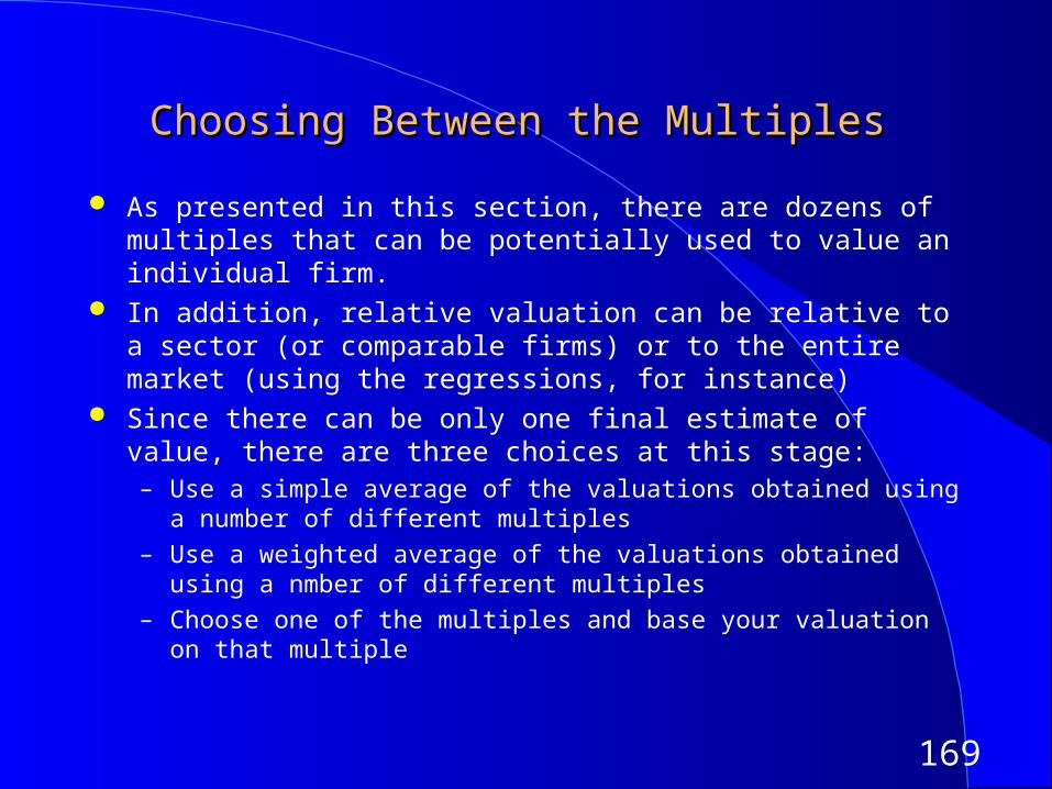
169

Choosing Between the MultiplesChoosing Between the Multiples

As presented in this section, there are dozens of multiples that can be potentially used to value an individual firm.

In addition, relative valuation can be relative to a sector (or comparable firms) or to the entire market (using the regressions, for instance)

Since there can be only one final estimate of value, there are three choices at this stage:– Use a simple average of the valuations obtained using a number of

different multiples

– Use a weighted average of the valuations obtained using a nmber of different multiples

– Choose one of the multiples and base your valuation on that multiple

170

Averaging Across MultiplesAveraging Across Multiples

This procedure involves valuing a firm using five or six or more multiples and then taking an average of the valuations across these multiples.

This is completely inappropriate since it averages good estimates with poor ones equally.

If some of the multiples are “sector based” and some are “market based”, this will also average across two different ways of thinking about relative valuation.

171

Weighted Averaging Across MultiplesWeighted Averaging Across Multiples

In this approach, the estimates obtained from using different multiples are averaged, with weights on each based upon the precision of each estimate. The more precise estimates are weighted more and the less precise ones weighted less.

The precision of each estimate can be estimated fairly simply for those estimated based upon regressions as follows:

Precision of Estimate = 1 / Standard Error of Estimate

where the standard error of the predicted value is used in the denominator.

This approach is more difficult to use when some of the estimates are subjective and some are based upon more quantitative techniques.

172

Picking one MultiplePicking one Multiple

This is usually the best way to approach this issue. While a range of values can be obtained from a number of multiples, the “best estimate” value is obtained using one multiple.

The multiple that is used can be chosen in one of two ways:– Use the multiple that best fits your objective. Thus, if you want the

company to be undervalued, you pick the multiple that yields the highest value.

– Use the multiple that has the highest R-squared in the sector when regressed against fundamentals. Thus, if you have tried PE, PBV, PS, etc. and run regressions of these multiples against fundamentals, use the multiple that works best at explaining differences across firms in that sector.

– Use the multiple that seems to make the most sense for that sector, given how value is measured and created.

173

Self Serving … But all too commonSelf Serving … But all too common

When a firm is valued using several multiples, some will yield really high values and some really low ones.

If there is a significant bias in the valuation towards high or low values, it is tempting to pick the multiple that best reflects this bias. Once the multiple that works best is picked, the other multiples can be abandoned and never brought up.

This approach, while yielding very biased and often absurd valuations, may serve other purposes very well.

As a user of valuations, it is always important to look at the biases of the entity doing the valuation, and asking some questions:– Why was this multiple chosen?

– What would the value be if a different multiple were used? (You pick the specific multiple that you want to see tried.)

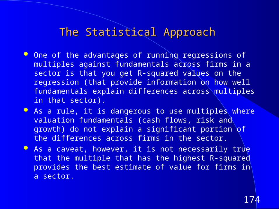
174

The Statistical ApproachThe Statistical Approach

One of the advantages of running regressions of multiples against fundamentals across firms in a sector is that you get R-squared values on the regression (that provide information on how well fundamentals explain differences across multiples in that sector).

As a rule, it is dangerous to use multiples where valuation fundamentals (cash flows, risk and growth) do not explain a significant portion of the differences across firms in the sector.

As a caveat, however, it is not necessarily true that the multiple that has the highest R-squared provides the best estimate of value for firms in a sector.

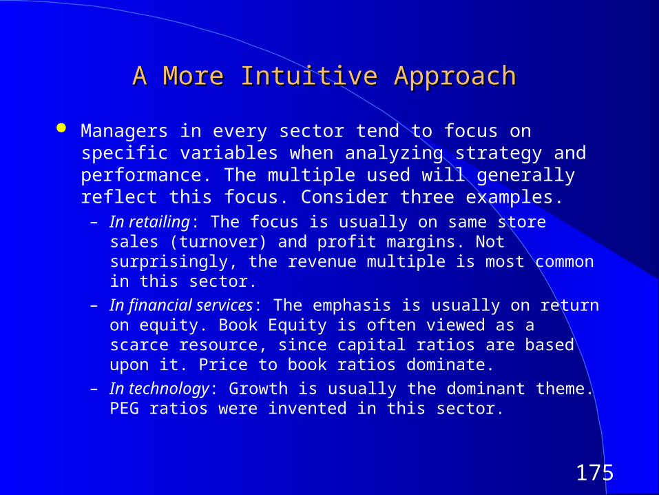
175

A More Intuitive ApproachA More Intuitive Approach

Managers in every sector tend to focus on specific variables when analyzing strategy and performance. The multiple used will generally reflect this focus. Consider three examples.– In retailing: The focus is usually on same store sales (turnover) and profit

margins. Not surprisingly, the revenue multiple is most common in this sector.

– In financial services: The emphasis is usually on return on equity. Book Equity is often viewed as a scarce resource, since capital ratios are based upon it. Price to book ratios dominate.

– In technology: Growth is usually the dominant theme. PEG ratios were invented in this sector.

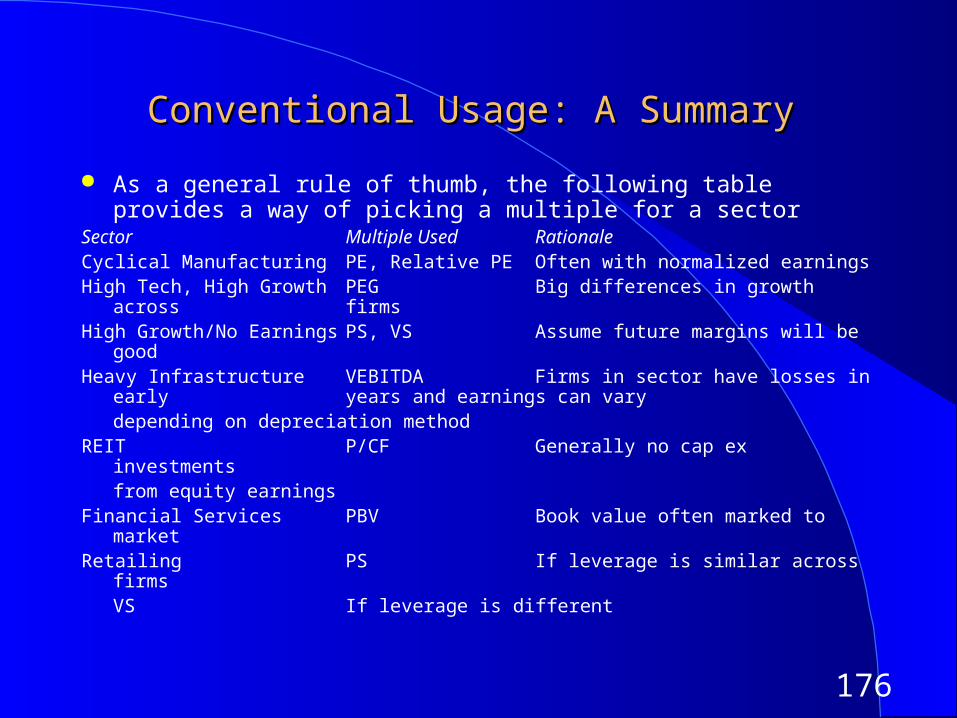
176

Conventional Usage: A SummaryConventional Usage: A Summary

As a general rule of thumb, the following table provides a way of picking a multiple for a sector

Sector Multiple Used RationaleCyclical Manufacturing PE, Relative PE Often with normalized earningsHigh Tech, High Growth PEG Big differences in growth across

firmsHigh Growth/No Earnings PS, VS Assume future margins will be goodHeavy Infrastructure VEBITDA Firms in sector have losses in early

years and earnings can varydepending on depreciation method

REIT P/CF Generally no cap ex investments from equity earnings

Financial Services PBV Book value often marked to marketRetailing PS If leverage is similar across firms

VS If leverage is different

177

Sector or Market MultiplesSector or Market Multiples

The conventional approach to using multiples is to look at the sector or comparable firms.

Whether sector or market based multiples make the most sense depends upon how you think the market makes mistakes in valuation– If you think that markets make mistakes on individual firm valuations but

that valuations tend to be right, on average, at the sector level, you will use sector-based valuation only,

– If you think that markets make mistakes on entire sectors, but is generally right on the overall market level, you will use only market-based valuation

It is usually a good idea to approach the valuation at two levels:– At the sector level, use multiples to see if the firm is under or over valued

at the sector level– At the market level, check to see if the under or over valuation persists

once you correct for sector under or over valuation.

178

A TestA Test

You have valued Earthlink Networks, an internet service provider, relative to other internet companies using Price/Sales ratios and find it to be under valued almost 50% .When you value it relative to the market, using the market regression, you find it to be overvalued by almost 50%. How would you reconcile the two findings?

One of the two valuations must be wrong. A stock cannot be under and over valued at the same time.

It is possible that both valuations are right.

What has to be true about valuations in the sector for the second statement to be true?

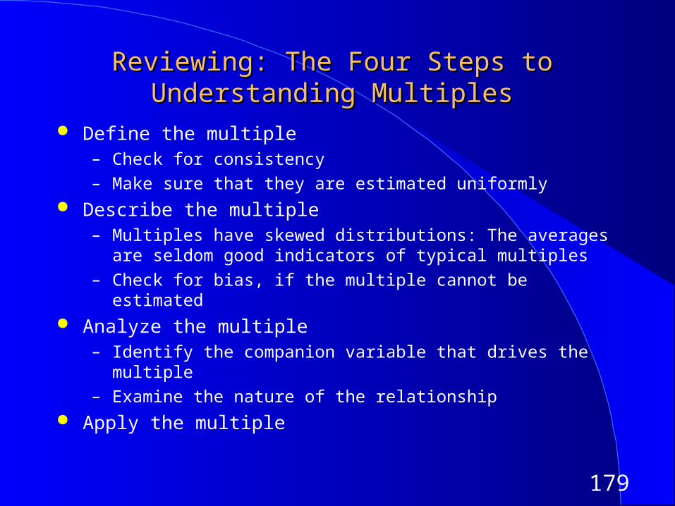
179

Reviewing: The Four Steps to Understanding Reviewing: The Four Steps to Understanding MultiplesMultiples

Define the multiple– Check for consistency

– Make sure that they are estimated uniformly Describe the multiple

– Multiples have skewed distributions: The averages are seldom good indicators of typical multiples

– Check for bias, if the multiple cannot be estimated Analyze the multiple

– Identify the companion variable that drives the multiple

– Examine the nature of the relationship Apply the multiple