1 directional cell search delay analysis for cellular
TRANSCRIPT

arX
iv:1
709.
0077
9v1
[cs
.IT
] 4
Sep
201
71
Directional Cell Search Delay Analysis for
Cellular Networks with Static Users
Yingzhe Li, Francois Baccelli, Jeffrey G. Andrews, Jianzhong Charlie Zhang
Abstract
Cell search is the process for a user to detect its neighboring base stations (BSs) and make a
cell selection decision. Due to the importance of beamforming gain in millimeter wave (mmWave)
and massive MIMO cellular networks, the directional cell search delay performance is investigated. A
cellular network with fixed BS and user locations is considered, so that strong temporal correlations
exist for the SINR experienced at each BS and user. For Poisson cellular networks with Rayleigh fading
channels, a closed-form expression for the spatially averaged mean cell search delay of all users is
derived. This mean cell search delay for a noise-limited network (e.g., mmWave network) is proved to
be infinite whenever the non-line-of-sight (NLOS) path loss exponent is larger than 2. For interference-
limited networks, a phase transition for the mean cell search delay is shown to exist in terms of the
number of BS antennas/beams M : the mean cell search delay is infinite when M is smaller than a
threshold and finite otherwise. Beam-sweeping is also demonstrated to be effective in decreasing the
cell search delay, especially for the cell edge users.
I. INTRODUCTION
Cell search is a critical prerequisite to establish an initial connection between a cellular
user and the cellular network. Specifically, the users will detect their neighboring BSs and
make the cell selection decision during a downlink cell search phase, after which the users
can acquire connections with the network by initiating an uplink random access phase. The
transmissions and receptions during cell search are performed omni-directionally in LTE [1],
but this is unsuitable for mmWave communication [2]–[5] or massive MIMO [6]–[9] due to the
lack of enough directivity gain. By contrast, directional cell search schemes that leverage BS
Y. Li, J. G. Andrews and F. Baccelli are with the Wireless Networking and Communications Group (WNCG), The University
of Texas at Austin (email: [email protected], [email protected], [email protected]). J. Zhang is with
Samsung Research America-Dallas (email: [email protected]). Date revised: November 1, 2021.

2
and/or user beam-sweeping to achieve extra directivity gains, can ensure reasonable cell search
performance [9]–[15]. In this paper, we leverage stochastic geometry [16]–[18] to develop an
analytical framework for the directional cell search delay performance of a fixed cellular network,
where the BS and user locations are fixed over a long period of time (e.g., more than several
minutes). We believe the analytical tools developed in this paper can provide useful insights
into practical fixed cellular networks such as fixed mmWave or massive MIMO broadband
networks [7], [19], [20], or mmWave backhauling networks [2], [21].
A. Related Work
Beam-sweeping is a useful method to improve cell search performance compared to conven-
tional omni-directional cell search for both mmWave and massive MIMO networks. Specifically,
mmWave links generally require high directionality with large antenna gains to overcome the
high isotropic path loss of mmWave propagation. As a result, in mmWave networks, applying
beam-sweeping for cell search not only provides sufficient signal-to-noise ratio (SNR) to create
viable communications, but also facilitates beam alignment between the BS and users [11]–
[13], [22]–[24]. The directional cell search delay performance of mmWave systems has been
investigated in [12], [22], [23] from a link level perspective, and in [13], [24] from a system level
perspective. In particular, [13] and [24] consider the user and mmWave BS locations are fixed
within an initial access cycle, but independently reshuffled across cycles. This block coherent
scenario is fundamentally different from that of a fixed network. For a massive MIMO system,
the BSs can achieve an effective power gain that scales with the number of antennas if the
channel state information (CSI) is known at the BSs [9]. However, since such an array gain is
unavailable for cell search operations due to the lack of CSI, the new users may be unable to join
the system using the traditional omnidirectional cell search [9], [14], [15]. In order to overcome
this issue, [15] has proposed open-loop beamforming to exhaustively sweep through BS beams
for cell search. This design has been implemented and verified on a sub-6 GHz massive MIMO
prototype [15], but the analytical directional cell search performance has not been investigated
for fixed cellular networks from a system level perspective.
Due its analytical tractability for cellular networks [16]–[18], stochastic geometry is a natural
candidate for analyzing the directional cell search delay in such fixed cellular networks. In
particular, stochastic geometry has already been widely used to investigate fixed Poisson network

3
performance through the local delay metric [16], [25]–[28], which characterizes the number of
time slots needed for the SINR to exceed a certain SINR level. In [16], [25], the local delay for
fixed ad hoc networks was found to be infinite under several standard scenarios such as Rayleigh
fading with constant noise. A new phase transition was identified for the interference-limited
case in terms of the mean local delay: the latter is finite when certain parameters are above a
threshold, and infinite otherwise. The local delay for noise-limited and interference-limited fixed
Poisson networks was also investigated in [26]–[28], where it is shown that power control is an
efficient method to ensure a finite mean local delay. These previous works mainly focused on
omni-directional communications.
B. Contributions
In this work, we analyze the cell search delay in fixed cellular networks with a directional cell
search protocol. We consider a time-division duplex (TDD) cellular system, where system time
is divided into different initial access (IA) cycles. Each cycle starts with the cell search period,
wherein BSs apply a synchronous beam-sweeping pattern to broadcast the synchronization
signals. A mathematical framework is developed to derive the exact expression for the mean
cell search delay, which quantifies the spatial average of the individual mean cell search delays
perceived by all users. The main contributions of this paper are summarized as follows.
Beam-sweeping is shown to reduce the number of IA cycles needed to succeed in cell
search. For any arbitrary BS locations and fading distribution, the mean number of initial access
cycles required to succeed in cell search is proved to be decreasing when the number of BS
antennas/beams is multiplied by a factor m > 1.
An exact expression for the mean cell search delay is derived for Poisson point process
(PPP) distributed BSs and Rayleigh fading channels. This expression is given by an infinite
series, based on which the following observations are obtained:
• Under the noise limited scenario (e.g., mmWave networks), we prove that as long as the
path loss exponent for NLOS path is larger than 2, the mean cell search delay is infinite,
irrespective of the BS transmit power and the BS antenna/beam number.
• Under the interference limited scenario (e.g., massive MIMO networks in sub-6 GHz bands),
there exists a phase transition for mean cell search delay in terms of the BS antenna/beam
number M . Specifically, the mean cell search delay is infinite when M is smaller than a

4
critical value and finite otherwise. This fact was never observed in the literature to the best
of our knowledge.
Cell search delay distribution is numerically evaluated. The conditional mean cell search
delay of a typical user given its nearest BS distance is derived for PPP distributed BSs and
Rayleigh fading channels. The distribution of this conditional mean cell search delay is also
numerically evaluated, and we observe that the cell search delay distribution is heavy-tailed. We
also show that increasing the number of BS antennas/beams can significantly reduce the cell
search delay for cell edge users.
Overall, this paper has shown that in fixed networks the mean cell search delay could be very
large due to the temporal correlations induced by common randomness. As a result, for fixed
cellular networks, system parameters including the number of BS antennas and/or BS intensity
need to be carefully designed for reasonable cell search delay performance to be achieved.
II. SYSTEM MODEL
In this work, we consider a cellular system that has carrier frequency fc and total system
bandwidth W . The BS transmit power is denoted by Pb, and the total thermal noise power
is denoted by σ2. In the rest of this section, we present the proposed directional cell search
protocol, location models, propagation assumptions, and the performance metrics.
A. Directional Cell Search Protocol
We consider a TDD cellular system as shown in Fig. 1, where system time is divided into
different initial access cycles with period T , and where τ denotes the OFDM symbol period.
Initial access refers to the procedures that establish an initial connection between a user and the
cellular network. It consists of two main steps: cell search on the downlink and random access
(RA) on the uplink. Specifically, by detecting the synchronization signals broadcasted by BSs
during cell search, a user can determine the presence of its neighboring BSs and make the cell
selection decision. Then the user can initiate the random access process to its desired serving BS
by transmitting a RA preamble through the shared random access channel, and it is successfully
connected to the network if the BS can decode the RA preamble without any collision. The
main focus of this work is the cell search performance, while the random access performance
will be incorporated in our future work.

5
Each BS is equipped with a large dimensional antenna array with M to support highly
directional communications. For analytical tractability, the actual antenna pattern is approximated
by a sectorized beam pattern, where the antenna gain is constant within the main lobe. In addition,
we assume a 0 side lobe gain for the BS, which is a reasonable approximation because the BS
uses a large dimensional antenna array with narrow beams, possibly with a front-to-back ratio
larger than 30 dB [29]. Each BS supports analog beamforming with a maximum of M possible
BF vectors, where the m-th (1 ≤ m ≤ M) beamforming (BF) vector corresponds to the main-
lobe, which has antenna gain M , and covers a sector area with angle [2πm−1M
, 2π mM) [30]. Each
user is assumed to have a single omni-directional antenna with unit antenna gain [15], [31].
In the cell search phase, each BS sweeps through all M transmit beamforming directions to
broadcast the synchronization signals, and each user is able to detect a BS with sufficiently small
miss detection probability (such as 1%) if the signal-to-interference-plus-noise ratio (SINR) of
the synchronization signal from that BS exceeds Γcs. All BSs transmit synchronously using the
same beam direction during every symbol, and the cell search delay within each IA cycle is
therefore Tcs = M × τ . When every BS transmits using the m-th (1 ≤ m ≤ M) BF direction,
the typical user can only receive from the BSs located inside the “BS sector”
S
(
o,2π(m− 1)
M+ π,
2πm
M+ π
)
, (1)
where we define the infinite sector domain centered at u ∈ R2 by:
S(u, θ1, θ2) = {x ∈ R2, s.t., ∠(x− u) ∈ [θ1, θ2)}. (2)
There are M such non-overlapping BS sectors during cell search, with the j-th (1 ≤ j ≤ M)
sector being S(o, 2π(j−1)M
, 2πjM
). We say a BS sector is detected during cell search if the typical
user is able to detect the BS that provides the smallest path loss (i.e., the closest BS) inside
this sector, where the path loss can be estimated from the beam reference signals [19]. After
cell search, the typical user selects the BS with the smallest path loss among all the detected
BS sectors as its serving BS. For simplicity, we neglect the scenario where the BS providing
the smallest path loss inside a BS sector is in deep fade and unable to be detected, while some
other BSs can be detected in the same sector. Such a scenario does not change the fundamental
trends regarding the finiteness of the mean cell search that will be detailed in Section III (e.g.
Theorem 3), but the corresponding analysis is significantly more complicated.

6
Initial access cycle n Initial access cycle n+1
CS period RA period CS period RA period
...
...
...
...
DL beam
DL beam
DL beampair M
pair 2
pair 1τ
time
Data transmission period Data transmission period
...... ......
...
...
...
...
DL beam
DL beam
DL beampair M
pair 2
pair 1τ
Fig. 1: Illustration of two initial access cycles and the timing structure.
TABLE I: Notation and Simulation Parameters
Symbol Definition Simulation Value
Φ, λ BS PPP and intensity λ = 100 BS/km2
Φu, λu User PPP and intensity λu = 1000 users/km2
Pb, Pu BS and user transmit power Pb = 30 dBm, Pu = 23 dBm
fc, B Carrier frequency and system bandwidth (fc, B) = (73, 1) GHz, (2, 0.2) GHz
W Total thermal noise power −174 dBm/Hz + 10 log10(B)M Number of BS antennas and BF directions supported at each BS
αL, αN Path loss exponents for dual-slope model (αL, αN) = (2.1, 3.3), (2.5, 2.5)CL, CN Path loss at close-in reference distance for dual-slope model (CL, CN) = (69.71, 69.71) dB,
(38.46, 38.46) dB
Rc Critical distance for dual-slope path loss model 50m
Γcs,Γra SINR threshold to detect synchronization signal and RA preamble (Γcs,Γra) = (−4,−4) dB
τ OFDM symbol period 14.3 µs, 71.4 µs
T Initial access cycle period 20 ms, 100 ms
SM(i) i-th BS sector, i.e., SM(i) = {x ∈ R2, s.t., ∠x ∈ [2π (i−1)M
, 2π iM)}
{xi0}
Mi=1 BS providing the smallest path loss to the typical user inside SM(i)
R0 Distance from typical user to its nearest BS
Lcs(M,λ) Number of IA cycles to succeed in cell search
Lcs(R0.M, λ) Mean number of IA cycles to succeed in cell search conditionally on R0
Dcs(M,λ) Cell search delay
B(x, r) (Bo(x, r)) Closed (open) ball with center x and radius r
B. Spatial Locations and Propagation Models
The BS locations are assumed to be a realization of a stationary point process Φ = {xi}i with
intensity λ. The user locations are modeled as a realization of a homogeneous PPP with intensity
λu, which is denoted by Φu = {ui}i. In this paper, a fixed network scenario is investigated where
the BS locations are fixed, and the users are either fixed or move with very slow speed such as
a pedestrian speed (e.g., less than 1 km/h) . As a result, the BS and user locations appear to be
fixed across different initial access cycles. This is fundamentally different from the high mobility
scenario investigated in [13], [24], which assumes the BS and user PPPs are independently re-

7
shuffled across every initial access cycles.
Without loss of generality, we can analyze the performance of a typical user u0 located at
the origin. This is guaranteed by Slivnyak’s theorem, which states that the property observed by
the typical point of a PPP Φ′
is the same as that observed by the point at origin in the process
Φ′
∪ {o} [32], [33].
A dual-slope, non-decreasing path loss function [34] is adopted, where the path loss for a link
with distance r is given by:
l(r) =
CLrαL, if r < RC ,
CNrαN , if r ≥ RC .
(3)
The dual slope path loss model captures the dependency of the path loss exponent on the link
distance for various network scenarios, such as ultra-dense [34] and mmWave networks [35].
In particular, (3) is referred to as the LOS ball blockage model for mmWave networks [34],
wherein αL and αN represent the LOS and NLOS path loss exponents, and CL and CN represent
the path loss at a close-in reference distance (e.g., 1 meter). We focus on the scenario where
αN ≥ max(αL, 2). If αL = αN = α and CL = CN = C, the dual slope path loss model reverts
to the standard single-slope path loss model.
Due to the adopted antenna pattern for BSs, the directivity gain between BS and user is M
when the BS beam is aligned with the user, and 0 otherwise. The fading effect for every BS-
user link is modeled by an i.i.d. random variable, whose complementary cumulative distribution
function (CCDF) is a decreasing function G(·) with support [0,∞). In addition, we assume the
IA cycle length is such that the fading random variables for a given link are also i.i.d. across
different cycles.
C. Performance Metrics
The main performance metrics investigated in this work are the number of IA cycles, and
the corresponding cell search delay for the typical user to discover its neighboring BSs and
determine a potential serving BS. Without loss of generality, the IA cycle 1 in Fig. 1 represents
the first IA cycle of the typical user. Denote by eM(n) the success indicator for cell search of
IA cycle n. The number of IA cycles for the typical user to succeed in cell search is therefore:
Lcs(M,λ) = inf{n ≥ 1 : eM(n) = 1}. (4)

8
Since analog beamforming is adopted at each BS, the cell search delay is defined as follows:
Dcs(M,λ) = (Lcs(M,λ)− 1)T +Mτ. (5)
Finally, Table I summarizes the notation, the definitions and the system parameters that will
be used in the rest of this paper1.
III. ANALYSIS FOR MEAN CELL SEARCH DELAY
In this section, the mean cell search delay performance for the typical user is investigated,
which corresponds to the cell search delay under the Palm expectation with respect to the user
PPP Φu (i.e., E0Φu[Dcs(M,λ)]). In fact, the Palm expectation can also be understood from its
ergodic interpretation, which states that for any user u ∈ Φu with cell search delay Dcs(u,M, λ),
the following relation is true:
E0Φu[Dcs(M,λ)] = lim
n→∞
1
Φu(B(0, n))
∑
k
1u∈B(0,n)Dcs(u,M, λ). (6)
Therefore, the mean cell search delay of the typical user can also be understood as the spatial
average of the individual cell search delays among all the users. For notational simplicity, we
will use E in the rest of this paper to denote the Palm expectation under the user PPP Φu.
A. Cell Search Delay Under General BS Deployment and Fading Assumptions
In this part, we first investigate the cell search delay under a general BS location model (not
necessarily PPP) and fading distribution. According to Section II, the BS and user locations
are fixed, and the fading variables for every link are i.i.d. across IA cycles. Therefore, given
the BS process Φ, the cell search success indicators for different IA cycles {eM(n)} form an
i.i.d. Bernoulli sequence of random variables. The cell search success probability is denoted by
πM(Φ) = E [eM(1)|Φ].
Since each BS sector can be independently detected given Φ, and cell search is successful if
at least one BS sector is detected. Conditionally on Φ, the cell search success probability for
1For the symbols with two simulation values, the first one is for the noise limited scenario, and the second one is for the
interference limited scenario, which will be detailed in Section IV.

9
every IA cycle is therefore:
πM (Φ) = 1−
M∏
i=1
[1− E [eM (i)|Φ]] , (7)
where eM(i) denotes the indicator that the BS providing the smallest path loss inside BS sector
i is detected. Specifically, if we denote by SM(i) , S(o, 2π(i−1)M
, 2πiM) the BS sector i, xi
0 the
BS providing the smallest path loss to the typical user in Φ ∩ SM(i), and by {F ij} the fading
random variables from BSs in SM(i) to the typical user, we have:
E [eM(i)|Φ] = P
(
F i0/l(‖x
i0‖)
∑
xij∈Φ∩SM (i)\{xi
0}F ij/l(‖x
ij‖) +W/PM
> Γcs
∣
∣
∣
∣
Φ
)
= E
[
G
(
Γcsl(‖xi0‖)(
∑
xij∈Φ∩SM (i)\{xi
0}
Fij/l(‖x
ij‖) +W/PM)
)∣
∣
∣
∣
Φ
]
, (8)
where the expectation in (8) is taken with respect to the i.i.d. fading random variables {F ij}.
In the following theorem, we derive the mean number of IA cycles for the typical user to
succeed in the cell search under the Palm expectation of the user process.
Theorem 1: The mean number of IA cycles needed for the typical user to succeed in cell
search is given by:
E[Lcs(M,λ)|Φ] =1
1−∏M
i=1 [1− E [eM(i)|Φ]], (9)
E[Lcs(M,λ)] = EΦ
[
1
1−∏M
i=1 [1− E [eM(i)|Φ]]
]
. (10)
Proof: The first part can be proved by the fact that given Φ, Lcs(M,λ) has a geometric dis-
tribution with success probability πM (Φ); while the second part follows by taking the expectation
of (9) with respect to Φ.
Remark 1: Since E [eM(i)|Φ] > 0 according to (8), the conditional mean cell search delay
E[Lcs(M,λ)|Φ] will be finite almost surely. However, the overall spatial averaged mean cell
search delay with respect to (w.r.t.) the BS PPP Φ (i.e. E[Lcs(M,λ)]) could be infinite under
certain network settings. This will be detailed in the next subsection.
A lower bound and an upper bound to E[Lcs(M,λ)] can be immediately obtained from (10),
which are provided in the following remarks.
Remark 2: By applying Jensen’s inequality to the positive random variable X and the function
10
f(x) = 1x
, we get that E[ 1X] ≥ 1
E[X]. Thus
E[Lcs(M,λ)] ≥1
1− E[
∏Mi=1 [1− E [eM (i)|Φ]]
] , (11)
where the equality holds when the BS PPP is independently re-shuffled across different IA cycles
from the typical user’s perspective, which coincides with the high mobility scenario considered
in [13], [24].
Remark 3: If we denote by x0 the BS providing the smallest path loss to the typical user, and
i∗ the index for the BS sector that contains x0, then∏M
j=1 [1− E [eM (j)|Φ]] ≤ 1−E [eM(i∗)|Φ].
Therefore, an upper bound to E[Lcs(M,λ)] is given by:
E[Lcs(M,λ)] ≤ E
[
1
E [eM(i∗)|Φ]
]
. (12)
Based on Theorem 1, we can prove the following relation between the BS antenna/beam
number M and the mean cell search delay.
Lemma 1: Given a realization of BS locations Φ, the mean number of IA cycles to succeed
in cell search is such that E[Lcs(M2, λ)|Φ] < E[Lcs(M1, λ)|Φ], if M2 = mM1 with m being an
integer larger than 1.
Proof: Since M2 = mM1, we know that SM1(i) =
⋃mj=1 SM2
((i−1)m+ j) for 1 ≤ i ≤ M1.
Denote by xi0 the BS providing the smallest path loss to the typical user inside Φ∩SM1
(i), and
assume xi0 ∈ Φ ∩ SM2
((i − 1)m + j0) for some j0 ∈ [1, m]. Due to the facts that M2 > M1,
SM2((i − 1)m + j0) ( SM1
(i), and since G(·) is a decreasing function, we get from (8) that
E [eM1(i)|Φ] < E [eM2
((i− 1)m+ j0)|Φ]. Also note that E [eM2((i− 1)m+ j)|Φ] > 0 for ∀j 6=
j0 according to (8), we hence have:
m∏
j=1
[1− E [eM2((i− 1)m+ j) |Φ]] < 1− E [eM2
(i)|Φ] . (13)
Thus the cell search success probability for the typical IA cycle satisfies:
πM2(Φ) = 1−
M2∏
i=1
[1− E [eM2(i)|Φ]]
= 1−
M1∏
i=1
(
m∏
j=1
[
1− E
[
eM2((i− 1)m+ j)
∣
∣
∣
∣
Φ
]]
)

11
> 1−
M1∏
i=1
[1− E [eM1(i)|Φ]] = πM1
(Φ). (14)
Finally the proof is concluded by applying Theorem 1.
Lemma 1 shows that for all BS location models and fading distributions, the conditional
number of IA cycles for cell search to succeed decreases when the number of BS antenna/beams
is multiplied by an integer m > 1, or equivalently when the BS beamwidth is divided by m.
This result also implies that E[Lcs(M2, λ)] ≤ E[Lcs(M1, λ)] if M2 = mM1.
Remark 4: In fact, Lemma 1 cannot be further extended. If M2 > M1 but M2/M1 is not an in-
teger, there will always exist special constructions of BS deployments such that E[Lcs(M2, λ)|Φ] >
E[Lcs(M1, λ)|Φ].
For the rest of this section, we investigate the mean cell search delay under several specific
network scenarios.
B. Mean Cell Search Delay in Poisson Networks with Rayleigh Fading
In this part, the BS locations are assumed to form a homogeneous PPP with intensity λ, and
the fading random variables are exponentially distributed with unit mean (i.e., G(x) = exp(−x)).
Due to its high analytical tractability, this network setting has been widely adopted to obtain the
fundamental design insights for conventional macro cellular networks [17], ultra-dense cellular
networks [34], and even mmWave cellular networks2 [35], [36].
Due to the PPP assumption for BSs, and the fact that different BS sectors are non-overlapping,
every BS sector can therefore be detected independently with the same probability. Since the
path loss function l(r) is non-decreasing, the BS that provides the minimum path loss to the
typical user inside the i-th BS sector Φ ∩ SM(i) (i.e., xi0) is the closest BS to the origin. The
angle of xi0 is uniformly distributed within [2π(i− 1)/M, 2πi/M), and the CCDF for the norm
of xi0 can be derived as follows:
P(‖xi0‖ ≥ r) = P
(
minx∈Φ∩SM (i)
‖x‖ ≥ r
)
= exp(−λπr2
M), (15)
where the second equality follows from the void probability for PPPs. Therefore, the probability
2The SINR and rate trends for mmWave networks under Rayleigh fading and PPP configured BSs have been shown to be
close to more realistic fading assumptions, such as the Nakagami fading or log-normal shadowing [11].

12
distribution function (PDF) for ‖xi0‖ is given by:
f‖xi0‖(r) =
2λπr
Mexp(−
λπr2
M). (16)
By applying Φ ∼ PPP(λ) and G(x) = exp(−x) into (8), the conditional detection probability
for the i-th BS sector is given by:
E [eM(i)|Φ] = E
[
exp
(
−Γcsl(‖xi0‖)
(
∑
xij∈Φ∩SM (i)\{xi
0}
Fij/l(‖x
ij‖) +W/PM
))∣
∣
∣
∣
Φ
]
= exp
(
−WΓcsl(‖x
i0‖)
PM
)
E
[
∏
xij∈Φ∩SM (i)\{xi
0}
exp
(
−Γcsl(‖xi0‖)F
ij/l(‖x
ij‖)
)]
(a)= exp
(
−WΓcsl(‖x
i0‖)
PM
)
∏
xij∈Φ∩SM (i)\{xi
0}
1
1 + Γcsl(‖xi0‖)/l(‖x
ij‖)
, FM(i,Φ), (17)
where step (a) is obtained by taking the expectation w.r.t. the fading random variables.
Theorem 2: If Φ ∼ PPP(λ), and the fading variables are exponentially distributed with unit
mean, the mean number of cycles for cell search to succeed is:
E[Lcs(M,λ)] =∞∑
j=0
AMj , (18)
where Aj = E[(1− FM(1,Φ))j ] is given by:
Aj =
∫ ∞
0
{ j∑
k=0
(−1)k(
j
k
)
exp
(
−WkΓcsl(r1)
PM
)
exp
(
−2πλ
M
∫ ∞
r1
(
1−1
(1 + Γcsl(r1)/l(r))k
)
rdr
)}
×2λπr1M
exp(−λπr21M
)dr1. (19)
Proof: By substituting (17) into Theorem 1, we obtain:
E[Lcs(M,λ)] = E
[
1
1−∏M
i=1 [1− FM(i,Φ)]
]
(a)= E
[ ∞∑
j=0
( M∏
i=1
[1− FM(i,Φ)]
)j]
(b)=
∞∑
j=0
E
[( M∏
i=1
[1− FM(i,Φ)]
)j]

13
(c)=
∞∑
j=0
{
E
[(
1− FM(1,Φ)
)j]}M
, (20)
where step (a) is derived from the fact that 11−x
=∑∞
j=0 xj for 0 ≤ x < 1, step (b) follows
from the monotone convergence theorem, and step (c) is because the events for BS sectors to
be detected are i.i.d. for PPP distributed BSs. Furthermore, we can compute Aj as follows:
E
[(
1− FM(1,Φ)
)j]
=
∫ ∞
0
E
[(
1− FM(1,Φ)
)j∣∣
∣
∣
x10 = (r1, 0)
]
2λπr1M
exp(−λπr21M
)dr
(a)=
∫ ∞
0
j∑
k=0
(−1)k(
j
k
)
Ex1
0
Φ
[
(FM (1,Φ))k∣
∣
∣
∣
Φ ∩ SM(1) ∩B(o, r1) = 0
]
2λπr1M
exp(−λπr21M
)dr
(b)=
∫ ∞
0
j∑
k=0
(−1)k(
j
k
)
E
[
exp
(
−WkΓcsl(r1)
PM
)
∏
xij∈Φ∩SM (i)∩Bc(o,r1)
1
(1 + Γcsl(r1)/l(‖xij‖))
k
]
×2λπr1M
exp(−λπr21M
)dr, (21)
where Ex1
0
Φ [·] in (a) denotes the expectation under the Palm distribution at BS x10; and step (b) is
derived from Slivnyak’s theorem. Finally the proof can be concluded by applying the probability
generating functional (PGFL) of PPPs [32] to (21).
Remark 5: Theorem 2 can be interpreted as E[Lcs(M,λ)] =∑∞
j=0 P(Lcs(M,λ) > j), with
AMj in (18) representing the probability that the BS sectors are not detected within j IA cycles,
i.e., P(Lcs(M,λ) > j).
Theorem 2 provides a series representation of the expected number of IA cycles to succeed
cell search. However, it is unclear from Theorem 2 whether E[Lcs(M)] is finite or not. In the
following, we will investigate the finiteness of E[Lcs(M,λ)] under two representative network
scenarios, namely the noise limited scenario and the interference limited scenario.
1) Noise limited Scenario: In the noise limited scenario, we assume the noise power dominates
the interference power (or interference power is perfectly canceled), such that only noise power
needs to be taken into account. Compared to conventional micro-wave cellular networks that
operate in sub-6 GHz bands, mmWave networks have much higher noise power due to the wider
bandwidth, and the interference power is much smaller due to the high isotropic path loss in
mmWave. As a result, mmWave cellular networks are typically noise limited, especially when

14
the carrier frequency and system bandwidth are high enough (e.g. 73 GHz carrier frequency with
2 GHz bandwidth) [35], [37].
Since the interference power is zero under the noise limited scenario, Theorem 2 becomes:
E[Lcs(M,λ)] =∞∑
j=0
{∫ ∞
0
(
1− exp
(
−WΓcsl(r1)
PM
))j2λπr1M
exp(−λπr21M
)dr1
}M
. (22)
Through the change of variable (v = λr2), (22) becomes
E[Lcs(M,λ)] =∞∑
j=0
{∫ ∞
0
(
1− exp
(
−WΓcsl(
√
(v/λ))
PM
)
)j2π
Mexp(−
πv
M)dv
}M
, (23)
which shows that E[Lcs(M,λ)] is non-increasing as the BS intensity λ increases, i.e., network
densification helps in reducing the number of IA cycles to succeed in cell search.
In the next two lemmas, we prove that the finiteness of E[Lcs(M,λ)] depends on the NLOS
path loss exponent αN , and that a phase transition for E[Lcs(M,λ)] happens when αN = 2.
Theorem 3: Under the noise limited scenario, for any finite number of BS antennas/beams
M and BS intensity λ, E[Lcs(M,λ)] = ∞ whenever the NLOS path loss exponent αN > 2.
Proof: Given the number of BS antennas/beams M and for any arbitrarily large positive
value v0 with v0 > Rc, we can re-write (22) to obtain the following lower bound on E[Lcs(M)]:
∞∑
j=0
{∫ ∞
0
(
1− exp
(
−WΓcsl(r1)
PM
))j2λπr1M
exp(−λπr21M
)dr1
}M
(a)
≥
∞∑
j=0
{∫ ∞
v0
(
1− exp
(
−WΓcsCNr
αN
1
PM
))j2λπr1M
exp(−λπr21M
)dr1
}M
>
∞∑
j=0
{(
1− exp
(
−WΓcsCNv
αN
0
PM
))j∫ ∞
v0
2λπr1M
exp(−λπr21M
)dr1
}M
=
∞∑
j=0
(
1− exp
(
−WΓcsCNv
αN
0
PM
))jM
exp(−λπv20)
=exp(−λπv20)
1− (1− exp(−WΓcsCNvαN
0 /PM))M
(b)
≥1
Mexp
(
WΓcsCNvαN
0 /PM − λπv20) v0→∞−→ ∞, (24)
where l(r1) = CNrαN
1 in step (a) because r1 ≥ v0 > Rc. Step (b) follows from the fact that for
any 0 ≤ x ≤ 1 and M ∈ N+, we have: (1 − x)M + xM ≥ 1, thus 11−(1−x)M
≥ 1xM
. Note that

15
since αN > 2, (24) goes to infinity when v0 goes to infinity, which completes the proof.
According to Lemma 3, the expected cell search delay is infinity whenever αN > 2, which
cannot be alleviated by BS densification (i.e., increase λ), or using a higher number of BS
antennas (i.e., increase M). The reason can be explained from (24), which shows that due to
the PPP-configured BS deployment, the typical user could be located at the “cell edge” with
its closest BS inside every BS sector farther than some arbitrarily large distance v. There is a
exp(−λπv2) fraction of such cell edge users, and the corresponding number of IA cycles required
for them to succeed in cell search is at least exp(CvαN ) for some C > 0. Therefore, the expected
cell search delay averaged over all the users will ultimately be infinite when αN > 2. From a
system level perspective, this indicates that for noise limited networks with αN > 2, there will
always be a significant fraction of cell edge users requiring a very large number of IA cycle to
succeed cell search, so that the spatial averaged cell search delay perceived by all users will be
determined largely by these cell edge users, which explains why an infinite mean cell search
delay is observed.
Theorem 4: Under the noise limited scenario with NLOS path loss exponent αN = 2, the
expected number of IA cycles to succeed in cell search E[Lcs(M,λ)] = ∞ if the BS density λ
and the BS antenna/beam number M satisfy λM < ΓcsCNWPπ
, and E[Lcs(M,λ)] < ∞ if λM >
ΓcsCNWPπ
, i.e., the phase transition for E[Lcs(M,λ)] happens at (λ∗,M∗) with λ∗M∗ = ΓcsCNWPπ
.
Proof: If αN = 2, it is clear from (24) that E[Lcs(M,λ)] = ∞ if λM < ΓcsCNWPπ
. In
addition, we can simplify the upper bound to E[Lcs(M,λ)] from Remark 3 under the noise
limited scenario, which is given as follows:
E[Lcs(M,λ)]
(a)
≤
∫ ∞
0
exp
(
WΓcsl(r0)
PM
)
λ2πr0 exp(−λπr20)dr0
=
∫ Rc
0
exp
(
WΓcsCLrαL
0
PM
)
λ2πr0 exp(−λπr20)dr0 +
∫ ∞
Rc
exp
(
WΓcsCNrαN
0
PM
)
λ2πr0 exp(−λπr20)dr0
< exp
(
WΓcsCLRαLc
PM
)(
1− exp(−λπR2c)
)
+
∫ ∞
Rc
exp
(
WΓcsCNrαN
0
PM
)
λ2πr0 exp(−λπr20)dr0,
(25)
where (a) is obtained by applying the noise limited assumption to (17), and noting that the BS
providing the smallest path loss among all the BSs is the closest BS of Φ to the origin. Since

16
αN = 2, it can be observed from (25) that E[Lcs(M)] is guaranteed to have a finite mean if
λM > ΓcsCNWPπ
.
We can observe from the proof of Lemma 4 that for any arbitrarily large distance r0, there
is a fraction exp(−λπr20) of cell edge users whose nearest BSs are farther than r0, and the
number of IA cycles for these edge users to succeed cell search scales as exp(WΓcsCN r2
0
PM). As
a result, if the BS deployment is too sparse or the number of BS antennas/beams is such that
λM < ΓcsCNWPπ
, the cell search delay averaged over all the users becomes infinity due to cell
edge users. By contrast, with network densification, the fraction of cell edge users with poor
signal power is reduced, and the average cell search delay can be reduced to a finite mean value
whenever λM > ΓcsCNWPπ
. A similar behavior happens when the BSs are using more antennas
to increase the SNR for the cell edge users.
To summarize, for the noise limited scenario such as a mmWave network, the mean cell search
delay is infinite whenever the NLOS path loss exponent αN > 2, which is typically the case.
However, for the special case with NLOS path loss exponent αN = 2, the mean cell search
delay could switch from infinity to a finite value through careful network design, such as BS
densification or adopting more BS antennas.
2) Interference limited Scenario: In the interference limited scenario, the noise power is
dominated by the interference power, so that we can assume W = 0. For example, a massive
MIMO network that operates in the sub-6 GHz bands is typically interference limited [6]. In
this part, we investigate the cell search delay in an interference-limited network with a standard
single slope path loss function l(r) = Crα, which is suitable for networks with sparsely deployed
BSs as opposed to ultra-dense networks [34].
First, we prove that Theorem 2 can be greatly simplified under this interference limited
scenario.
Lemma 2: Under the interference limited scenario, the expected number of initial access
cycles required to succeed in cell search is given by:
E[Lcs(M)] =∞∑
j=0
( j∑
k=0
(−1)k(
jk
)
1 + 2∫ +∞1
(1− (1 + Γcs/rα)−k)rdr
)M
. (26)
Proof: By substituting W = 0 and l(r) = Crα into (19), Aj defined in (19) can be further

17
simplified as follows:
Aj =
∫ ∞
0
{ j∑
k=0
(−1)k(
j
k
)
exp
(
−2πλ
M
∫ ∞
r1
(
1−1
(1 + Γcsrα1 /r
α)k
)
rdr
)}
2λπr1M
exp(−λπr21M
)dr1
=
j∑
k=0
(−1)k(
j
k
){∫ ∞
0
exp
(
−2πλr21M
∫ ∞
1
(
1−1
(1 + Γcs/rα)k
)
rdr
)
2λπr1M
exp(−λπr21M
)dr1
}
=
j∑
k=0
(−1)k(
jk
)
1 + 2∫ +∞1
(1− (1 + Γcs/rα)−k)rdr,
which completes the proof.
Remark 6: We can observe from Lemma 2 that E[Lcs(M)] does not depend on the BS
intensity λ under the interference limited scenario. This is because the increase and decrease of
the signal power can be perfectly counter-effected by the corresponding increase and decrease
of the interference power [17]. Another immediate observation from Lemma 2 is that Aj is
independent of the number of BS antennas M for ∀j. Since Aj ≤ 1 according to its definition
in Theorem 2, E[Lcs(M)] is therefore monotonically non-increasing with respect to M , which
is a stronger observation than Lemma 1.
Remark 7: If the path loss exponent α = 2, it can be proved from Lemma 2 that E[Lcs(M)] =
∞ for ∀M . This is mainly because the interference power will dominate the signal power when
α = 2, so that the coverage probability is 0 for any SINR threshold Γcs.
If α > 2, we can prove that there may exist a phase transition for E[Lcs(M)] in terms of the
BS beam number M . In order to show that, we first apply Remark 3 and obtain a sufficient
condition to guarantee the finiteness for E[Lcs(M)].
Lemma 3: Under the interference limited scenario with path loss exponent α > 2, the expected
number of IA cycles to succeed cell search is such that E[Lcs(M)] < ∞ if the number of BS
beams is such that M > 2Γcs
α−2, where Γcs denotes the detection threshold for a BS. In particular,
when M = 1, i.e., the BS is omni-directional, E[Lcs(1)] is finite if and only if α > 2Γcs + 2.
Proof: Denote by x0 the closest BS to the origin among Φ, and SM(i∗) the BS sector
containing x0, we can obtain an upper bound to E[Lcs(M)] by substituting (17) and W = 0 into
Remark 3 as follows:
E[Lcs(M)] ≤ E
[
∏
xj∈Φ∩SM (i∗)\{x0}
(
1 + Γcsl(‖x0‖)/l(‖xj‖)
)]

18
(a)=
∫ ∞
0
E
[
∏
xj∈Φ∩SM (i∗)∩Bc(o,r0)
(
1 + Γcsl(r0)/l(‖xj‖)
)]
2λπr0 exp(−λπr20)dr0
(b)=
∫ ∞
0
exp
(
2πλΓcs
M
∫ ∞
r0
l(r0)r
l(r)dr
)
2λπr0 exp(−λπr20)dr0
(c)=
∫ ∞
0
exp
(
−
(
1−2Γcs
M(α− 2)
)
v
)
dv
=
∞, if M ≤ 2Γcs
α−2,
M(α−2)M(α−2)−2Γcs
, if M > 2Γcs
α−2,
(27)
where (a) is obtained by noting that x0 is the closest BS to the origin, (b) follows from the
PGFL for the PPP3, and (c) is derived through change of variables (i.e. v = λπr20). It can be
observed that (27) is finite whenever M > 2Γcs
α−2, which is a sufficient condition for the finiteness
of E[Lcs(M)]. In particular, the equality holds in the first step of (27) when M = 1. As a result,
E[Lcs(1)] is finite if and only if α > 2Γcs + 2.
According to Lemma 2 and Lemma 3, the number of IA cycles to succeed in cell search (i.e.,
E[Lcs(M)]) may have a phase transition in terms of the number of BS beams M , depending on
the relation between the path loss exponent α and the detection threshold Γcs. This is detailed
in the following theorem.
Theorem 5: The number of IA cycles to succeed in cell search for the interference limited
networks satisfy the following:
• If α > 2 + 2Γcs, E[Lcs(M)] < ∞ for the omni-directional BS antenna case, i.e., M = 1.
By the monotonicity of E[Lcs(M)] with respect to M , E[Lcs(M)] is guaranteed to be finite
for any M ≥ 1.
• If α ≤ 2+2Γcs, E[Lcs(M)] = ∞ for M = 1, and E[Lcs(M)] < ∞ if M > 2Γcs
α−2. Therefore,
according to the monotonicity of E[Lcs(M)], there exists a phase transition at M∗ ∈ [2, 2Γcs
α−2],
such that E[Lcs(M)] = ∞ for M ≤ M∗, and E[Lcs(M)] < ∞ for M > M∗. In particular,
E[Lcs(M)] = ∞ for ∀M if α = 2, which means M∗ = ∞.
The path loss exponent α depends on the propagation environment, and α = 2 corresponds to
a free space LOS scenario; while α increases as the environment becomes relatively more lossy
and scatter-rich, such as urban and suburban areas. In addition, the SINR detection threshold Γcs
3Note that [38, Theorem 4.9] does not directly apply to the PGFL calculation here since f(x) = 1+Γcsl(r0)/l(x) is larger than
1. However, we can use dominated convergence theorem to prove that for PPP Φ with intensity measure Λ(·), the PGFL result
still holds if function f(x) satisfies f(x) ≥ 1 and∫R2(f(x)−1)Λ(dx) < ∞, i.e. E[
∏xi∈Φ
f(xi)] = exp(∫R2(f(x)−1)Λ(dx).

19
depends on the receiver decoding capability, which is typically within −10 dB and 0 dB [12].
Theorem 5 shows that in a lossy environment with α > 2 + 2Γcs, the typical user can detect
a nearby BS in a finite number of IA cycles on average. This is mainly because the relative
strength of the useful signal with respect to the interfering signals is strong enough. However,
when α ≤ 2 + 2Γcs, E[Lcs(M)] could be infinite due to the significant fraction of cell edge
users that have poor SIR coverage and therefore require a very high number of IA cycles to
succeed in cell search. Specifically, when M is very small (e.g., M = 1), the edge user is subject
to many strong nearby interferers inside every BS sector, so that the corresponding cell search
delay averaged over all users becomes infinity. However, as M increases, the BS beam sweeping
will create enough angular separation so that the nearby BSs to the edge user could locate in
different BS sectors. As a result, Lcs(M) is significantly decreased for cell edge users as M
increases, and therefore the phase transition for E[Lcs(M)] happens.
In summary, for an interference-limited network, we can always ensure the network to be in a
desirable condition with finite mean cell search delay by tuning the number of BS beams/antennas
M appropriately.
C. Cell Search Delay Distribution in Poisson Networks with Rayleigh Fading
The previous part is mainly focused on the mean number of IA cycles to succeed in cell search
E[Lcs(M,λ)], or equivalently the mean cell search delay. However, as shown in Theorem 3,
Theorem 4 and Theorem 5, E[Lcs(M,λ)] could be infinite under various settings, and there are
large variations of the performance between cell edge user and cell center user. Therefore, it is
also important to analyze the cell search delay distribution for system design.
Since the cell search delay Dcs(M,λ) depends on the spatial point process model for BSs
and the fading random variables at each IA cycle, its distribution is intractable in general. In
this section, we evaluate the distribution of the conditional mean cell search delay given the
distance from the typical user to its closest BS R0, which is a random variable with PDF
fR0(r0) = 2πλr0 exp(−λπr20). Specifically, we first derive the expected number of IA cycles to
succeed in cell search given R0, i.e., E[Lcs(M,λ)|R0], which is a function of random variable R0
with mean E[Lcs(M,λ)]. For notation simplicity, we denote by Lcs(R0,M, λ) , E[Lcs(M,λ)|R0]
for the rest of the paper. According to (5), we will evaluate the distribution of the following

20
conditional mean cell search delay:
Dcs(R0,M, λ) , (Lcs(R0,M, λ)− 1)T +Mτ. (28)
The main reason to investigate the cell search delay conditionally on R0 is because R0 captures
the location and therefore the signal quality of the typical user. In particular, R0 ≪ 12√λ
corresponds to the cell center user, while R0 ≫ 12√λ
corresponds to the cell edge user, where
12√λ
represents the mean distance from the typical user to its nearest BS on the PPP Φ.
In order to derive Lcs(R0,M, λ) in (28), we will first derive E[Lcs(M,λ)|R1, R2, ..., RM ],
where Ri denotes the distance from the typical user to its closest BS in the i-th BS sector (i.e.,
Ri = ‖xi0‖) for 1 ≤ i ≤ M .
Lemma 4: Given the distances from the typical user to its nearest BSs inside every BS sector
R1, ..., RM , the mean number of IA cycles for cell search is:
E[Lcs(M,λ)|R1, R2, ..., RM ] =∞∑
j=0
M∏
i=1
fj(Ri,M, λ), (29)
where fj(Ri) denotes the probability that xi0 is detected in the first j IA cycles, which is:
fj(Ri,M, λ) =
j∑
k=0
(−1)k(
j
k
)
exp
(
−WkΓcsl(Ri)
PM
)
exp
(
−2λπ
M
∫ ∞
Ri
(1−1
(1 + Γcsl(Ri)/l(r))k)rdr
)
.
Proof: We can first prove E[Lcs(M,λ)|R1, R2, ..., RM ] = E[E[Lcs(M,λ)|Φ]|R1, R2, ..., RM ],
which is due to the tower property for conditional expectations. The rest of the proof follows
steps similar to those of Theorem 2, and therefore we omit the details.
Next we prove the following corollary to derive Lcs(R0,M, λ) from E[Lcs(M,λ)|R1, R2, ..., RM ].
Corollary 1: For all i.i.d. non-negative random variables R1, R2,...,RM with CCDF G(r), and
all functions F : [0,∞)M → [0,∞) which are symmetric, the following relation holds true:
E[F (R1, R2, ..., RM)|min(R1, R2, ..., RM) = r] =E[F (r, R2, ..., RM)1{Rj>r,∀j 6=1}]
(G(r))M−1. (30)
Proof: Denote by R0 = min(R1, R2, ..., RM), then we can obtain (30) as follows:
E[F (R1, R2, ..., RM)|R0 = r]
= limǫ→0
E[F (R1, R2, ..., RM)× 1|R0−r|<ǫ]
P(|R0 − r| < ǫ)

21
= limǫ→0
∑Mi=1 E[F (R1, R2, ..., RM)× 1({|Ri−r|<ǫ}∩{Rj>Ri,∀j 6=i})]∑M
k=1 P({|Rk − r| < ǫ} ∩ {Rj > Rk, ∀j 6= k})
= limǫ→0
∑Mi=1 E[F (R1, R2, ..., RM)1({Rj>Ri,∀j 6=i})||Ri − r| < ǫ]∑M
k=1 P({Rj > Rk, ∀j 6= k}||Rk − r| < ǫ)
=
∑Mi=1E[F (R1, R2, ..., RM)1({Rj>Ri,∀j 6=i})|Ri = r]∑M
k=1 P({Rj > Rk, ∀j 6= k}|Rk = r),
the proof is completed by noting F is symmetric.
By taking F (R1, R2, ..., RM) = E[Lcs(M,λ)|R1, R2, ..., RM ] in Corollary 1, E[Lcs(M,λ)|R0]
can directly obtained as follows.
Lemma 5: Given the distance from the typical user to the nearest BS R0, the mean number
of IA cycles to succeed cell search is:
Lcs(R0,M, λ) =
∞∑
j=0
fj(R0,M, λ)
{∫ ∞
R0
fj(r,M, λ)λ2πr
Mexp(−
λπr2
M)dr
}M−1
exp
(
λπ(M − 1)R20
M
)
,
where the function fj(r,M, λ) is defined in Lemma 4.
Lemma 5 provides a method to evaluate the cell search delay distribution under a general
setting. For noise limited networks and interference limited networks, we can obtain the following
simplified results.
Corollary 2: For the noise limited network, Lcs(R0,M, λ) is given by:
Lcs(R0,M, λ) =
∑∞j=0(1− exp(−
ΓcsWCNRαN0
PM))j{
∫∞R0
(1− exp(−ΓcsWCNrαN
PM))j
×λ2πrM
exp(−λπr2
M)dr}M−1 exp(λπM−1
MR2
0), if R0 ≥ Rc,∑∞
j=0(1− exp(−ΓcsWCLR
αL0
PM))j{
∫∞RC
(1− exp(−ΓcsWCNrαN
PM))j
×λ2πrM
exp(−λπr2
M)dr +
∫ RC
R0
(1− exp(−ΓcsWCLrαL
PM))j
×λ2πrM
exp(−λπr2
M)dr}M−1 exp(λπM−1
MR2
0), if R0 < Rc.
(31)
Corollary 2 can be easily proved from Lemma 5 and the fact that interference power is 0.
Corollary 3: For the interference limited network and the standard single-slope path loss
model with path loss exponent α > 2, Lcs(R0,M, λ) is given by:
Lcs(R0,M, λ) =
∞∑
j=0
{ j∑
k=0
(−1)k(
j
k
)
exp
(
−2πλR2
0H(k, α,Γcs)
M
)}

22
×
{ j∑
k=0
(−1)k(
jk
)
exp
(
−2πλR2
0H(k,α,Γcs)
M
)
1 + 2H(k, α,Γcs)
}M−1
, (32)
where H(k, α,Γcs) =∫∞1(1− 1
(1+Γ/rα)k)rdr.
Proof: Since W = 0 and l(r) = Crα, fj(Ri,M, λ) in Lemma 5 can be simplified as:
fj(Ri,M, λ) =
j∑
k=0
(−1)k(
j
k
)
exp
(
−2πλR2
0H(k, α,Γcs)
M
)
. (33)
Therefore, we can further obtain that:
∫ ∞
R0
fj(r,M, λ)λ2πr
Mexp(−
λπr2
M)dr =
j∑
k=0
(−1)k(
j
k
)
exp(−λπM(1 + 2H(k, α,Γcs))R
20)
1 + 2H(k, α,Γcs). (34)
The proof can be completed by substituting (33) and (34) into Lemma 5.
IV. NUMERICAL EVALUATIONS
In this section, the distribution of the conditional mean cell search delay (28) is numerically
evaluated for both the noise limited scenario and the interference limited scenario. Specifically,
for the noise limited scenario, we consider a cellular network operating in the mmWave band
with carrier frequency fc = 73 GHz, bandwidth B = 2 GHz, and BS intensity λ = 100 BS/km2.
The path loss exponents for LOS and NLOS links are 2.1 and 3.3 respectively, and the critical
distance is Rc = 50m. In addition, the OFDM symbol period is τ = 14.3 µs, and the IA cycle
length is chosen as T = 20 ms [13], [19]. As for the interference limited scenario, we consider
a cellular network with carrier frequency fc = 2 GHz, BS intensity λ = 100 BS/km2, and a
standard single slope path loss model with path loss exponent α = 2.5. The OFDM symbol
period is τ = 71.4 µs, and the IA cycle length is T = 100 ms.
A. Conditional Expected Number of Cycles to Succeed in Cell Search
In order to evaluate the distribution of the conditional mean cell search delay, we first illustrate
Lemma 5. Specifically, we have simulated the cellular network with the directional cell search
protocol proposed in Section II-A, given the distance from the user to its nearest BS R0. As
shown in Lemma 3 and Remark 5, the cell edge users will require a large number of cycles to
succeed in cell search. Therefore, we have set an upper bound for the number of cycles that a
user can try cell search, which is equal to 1500 cycles for the noise limited scenario and 100

23
0 50 100 150R
0 (m)
0
500
1000
1500E
[Lcs
(M,
)|R
0]
M = 4, = 90°
M = 8, = 45°
M = 18, = 20°
M = 36, = 10°
fc = 73 GHz, B = 2 GHz
= 100 BS/km2, Rc = 50m
L = 2.1,
N = 3.3
Lines: theoryMarkers: simulation
(a) Noise limited networks
0 50 100 150R
0 (m)
1
1.5
2
2.5
3
3.5
4
4.5
5
E[L
cs(M
,)|
R0]
M = 4, = 90°
M = 8, = 45°
M = 12, = 30°
M = 18, = 20°
Lines: theoryMarkers: simulation
= 100 BS/km 2, = 2.5
(b) Interference limited networks
Fig. 2: Conditional expected number of cycles to succeed in cell search.
cycles for the interference limited scenario. Specifically, the infinite summation in Lemma 3 is
computed up to the 1500-th (100-th) term, and the simulation will treat a user as in outage if it
cannot be connected within 1500 (100) cycles.
Fig. 2 shows a close match between the analytical results and simulation results for both the
noise and interference limited scenarios, which is in line with Lemma 5. In addition, we can also
observe from Fig. 2 that the conditional expected number of cycles to succeed in cell search is
monotonically decreasing as the number of BS antennas/beams M increases, or as the distance
to the nearest BS R0 decreases.
B. Cell Search Delay Distribution in Noise Limited Networks
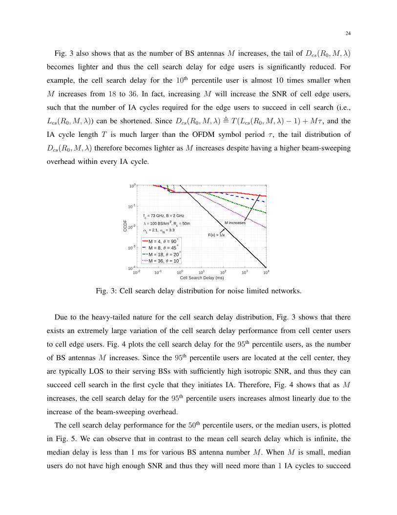
The cell search delay distribution for noise limited networks is numerically evaluated in this
part. Fig. 3 plots the CCDF of the conditional mean cell search delay Dcs(R0,M, λ), which is
obtained by generating 106 realizations of R0 and computing the corresponding Dcs(R0,M, λ)
through Corollary 2. We can observe from Fig. 3 that under the log-log scale, the tail distribution
function of Dcs(R0,M, λ), i.e., P(Dcs(R0,M, λ) ≥ t), decreases almost linearly with respect to t.
This indicates that the cell search delay is actually heavy-tailed and of the Pareto type. It can also
be observed from Fig. 3 that the tail distribution function satisfies limt→∞− log P(Dcs(R0,M,λ)≥t)
log t< 1
for M = 4, 8, 18, 36. Therefore, the expected cell search delay is always infinite, which is in
line with Lemma 3.
24
Fig. 3 also shows that as the number of BS antennas M increases, the tail of Dcs(R0,M, λ)
becomes lighter and thus the cell search delay for edge users is significantly reduced. For
example, the cell search delay for the 10th percentile user is almost 10 times smaller when
M increases from 18 to 36. In fact, increasing M will increase the SNR of cell edge users,
such that the number of IA cycles required for the edge users to succeed in cell search (i.e.,
Lcs(R0,M, λ)) can be shortened. Since Dcs(R0,M, λ) , T (Lcs(R0,M, λ)− 1) +Mτ , and the
IA cycle length T is much larger than the OFDM symbol period τ , the tail distribution of
Dcs(R0,M, λ) therefore becomes lighter as M increases despite having a higher beam-sweeping
overhead within every IA cycle.
10-2 10-1 100 101 102 103 104
Cell Search Delay (ms)
10-4
10-3
10-2
10-1
100
CC
DF
M = 4, = 90°
M = 8, = 45°
M = 18, = 20°
M = 36, = 10°
fc = 73 GHz, B = 2 GHz
= 100 BS/km2, Rc = 50m
L = 2.1,
N = 3.3
F(x) = 1/x
M increases
Fig. 3: Cell search delay distribution for noise limited networks.
Due to the heavy-tailed nature for the cell search delay distribution, Fig. 3 shows that there
exists an extremely large variation of the cell search delay performance from cell center users
to cell edge users. Fig. 4 plots the cell search delay for the 95th percentile users, as the number
of BS antennas M increases. Since the 95th percentile users are located at the cell center, they
are typically LOS to their serving BSs with sufficiently high isotropic SNR, and thus they can
succeed cell search in the first cycle that they initiates IA. Therefore, Fig. 4 shows that as M
increases, the cell search delay for the 95th percentile users increases almost linearly due to the
increase of the beam-sweeping overhead.
The cell search delay performance for the 50th percentile users, or the median users, is plotted
in Fig. 5. We can observe that in contrast to the mean cell search delay which is infinite, the
median delay is less than 1 ms for various BS antenna number M . When M is small, median
users do not have high enough SNR and thus they will need more than 1 IA cycles to succeed

25
5 10 15 20 25 30 35Number of BS Beams
0
0.1
0.2
0.3
0.4
0.5
0.6
95-t
h P
erce
ntile
Cel
l Sea
rch
Del
ay (
ms) f
c = 73 GHz, B = 2 GHz
= 100 BS/km2, Rc = 50m
L = 2.1,
N = 3.3
Fig. 4: 95th percentile cell search delay for noise limited network.
in cell search. As M increases, the cell search delay for median users first decreases due to the
improved SNR and cell search success probability, until the median users could succeed cell
search in the first cycle that they initiates IA. Then the cell search delay will increase as M is
further increased, which is because the beam sweeping overhead becomes more dominant. The
optimal BS antenna number M is 12 (or 30◦ beamwidth) in Fig. 5, which corresponds to a cell
search delay of 0.31 ms.
5 10 15 20 25 30 35Number of BS Beams
0.3
0.35
0.4
0.45
0.5
0.55
50-t
h P
erce
ntile
Cel
l Sea
rch
Del
ay (
ms)
fc = 73 GHz, B = 2 GHz
= 100 BS/km2, Rc = 50m
L = 2.1,
N = 3.3
Fig. 5: 50th percentile cell search delay for noise limited network.
C. Cell Search Delay Distribution in Interference Limited Networks
Similar to the noise limited scenario, we have evaluated the CCDF of cell search delay for
the interference limited scenario in Fig. 6 by generating 106 realizations of R0 and computing
the corresponding Dcs(R0,M, λ) through Corollary 3.

26
Fig. 6 shows that the tail distribution function of Dcs(R0,M, λ) decreases almost linearly
under the log-log scale, which means the distribution of Dcs(R0,M, λ) is also heavy-tailed
under the interference limited scenario. However, in contrast to the noise limited scenario where
the overall mean cell search delay is always infinite, the phase transition for mean cell search
delay of the interference limited scenario can be observed from Fig. 6. Specifically, when the
cell search is performed omni-directionally (i.e., M = 1), Fig. 6 shows that the decay rate of the
tail satisfies limt→∞− log P(Dcs(R0,M,λ)≥t)
log t< 1, which indicates an infinite mean cell search delay.
As M increases to 4, 8, 12, Fig. 6 shows that limt→∞− log P(Dcs(R0,M,λ)≥t)
log t> 1, which leads to
a finite mean cell search delay. This observation is consistent with Theorem 5, which shows
that for the considered interference limited scenario with path loss exponent α = 2.5 and SINR
detection threshold Γcs = −4 dB, the mean cell search delay is infinite when M = 1, and finite
as long as M > 1.59.
It can also be observed from Fig. 6 that BS beam-sweeping can significantly reduce the cell
search delay for both the median users and edge users in the interference limited networks. For
example, when the number of BS antennas/beams M is 1, 4, 8, and 12, the corresponding cell
search delay for the 50th percentile user is 200 ms, 8.98 ms, 1.18 ms, and 0.9123 ms respectively,
while the corresponding cell search delay for the 10th percentile user is 3720 ms, 53.84 ms, 5.14
ms and 1.35 ms respectively. The main reason for such a performance gain in the interference-
limited network is that as M increases, beam-sweeping creates more angular separations from
the nearby BSs to the user, so that the number of IA cycles to succeed in cell search can be
effectively reduced, especially for edge users.
10-1 100 101 102 103 104
Cell Search Delay (ms)
10-4
10-3
10-2
10-1
100
CC
DF
M = 1, omniM = 4, = 90°
M = 8, = 45°
M = 12, = 30°
= 100 BS/km2, = 2.5T = 100ms, = 71.4 s
F(x) = 1/x
Fig. 6: Cell search delay distribution for interference limited network.

27
V. CONCLUSIONS
This paper has proposed a mathematical framework to analyze the directional cell search
delay for fixed cellular networks, where the BS and user locations are static. Conditioned on the
BS locations, we have first derived the conditional expected cell search delay under the Palm
distribution of the user process. By utilizing a Taylor series expansion, we have further derived
the exact expression for the overall mean cell search delay in a Poisson cellular network with
Rayleigh fading channels. Based on this expression, the expected cell search delay in noise-
limited network was proved to be infinite when the NLOS path loss exponent is larger than
2. By contrast, a phase transition for the expected cell search delay in the interference-limited
network was identified: the delay is finite when the number of BS beams/antennas is greater than
a threshold, and infinite otherwise. Finally, by investigating the distribution of the conditional
cell search delay given the distance to the nearest BS, the cell search delay for the edge user
was shown to be significantly reduced as the number of BS beams/antennas increases, which
holds true for both the noise and interference limited networks.
The framework developed in this paper provides a tractable approach to handle the spatial
and temporal correlations of user’s SINR process in cellular networks with fixed BS and user
locations. Future work will leverage the proposed framework to derive the random access phase
performance, the overall expected initial access delay, as well as the downlink throughput
performance for such fixed cellular networks. In addition, we will also extend the framework to
incorporate user beamforming or power control.
ACKNOWLEDGMENTS
This work is supported in part by the National Science Foundation under Grant No. NSF-
CCF-1218338 and an award from the Simons Foundation (#197982), both to the University of
Texas at Austin.
REFERENCES
[1] E. Dahlman, S. Parkvall, and J. Skold, 4G: LTE/LTE-advanced for mobile broadband. Elsevier Science, 2011.
[2] Z. Pi and F. Khan, “An introduction to millimeter-wave mobile broadband systems,” IEEE Communications Magazine,
vol. 49, pp. 101–107, Jun. 2011.
[3] T. S. Rappaport, S. Sun, R. Mayzus, H. Zhao, Y. Azar, K. Wang, G. N. Wong, J. K. Schulz, M. Samimi, and F. Gutierrez,
“Millimeter wave mobile communications for 5G cellular: It will work!,” IEEE Access, vol. 1, pp. 335–349, May 2013.

28
[4] W. Roh, J.-Y. Seol, J. Park, B. Lee, J. Lee, Y. Kim, J. Cho, K. Cheun, and F. Aryanfar, “Millimeter-wave beamforming as an
enabling technology for 5G cellular communications: theoretical feasibility and prototype results,” IEEE Communications
Magazine, vol. 52, pp. 106–113, Feb. 2014.
[5] A. Ghosh, T. Thomas, M. C. Cudak, R. Ratasuk, P. Moorut, F. W. Vook, T. S. Rappaport, G. R. MacCartney, S. Sun,
S. Nie, et al., “Millimeter-wave enhanced local area systems: A high-data-rate approach for future wireless networks,”
IEEE Journal on Selected Areas in Communications, vol. 32, pp. 1152–1163, Jul. 2014.
[6] T. L. Marzetta, “Noncooperative cellular wireless with unlimited numbers of base station antennas,” IEEE Transactions
on Wireless Communications, vol. 9, pp. 3590–3600, Nov. 2010.
[7] E. G. Larsson, O. Edfors, F. Tufvesson, and T. L. Marzetta, “Massive MIMO for next generation wireless systems,” IEEE
Communications Magazine, vol. 52, pp. 186–195, Feb. 2014.
[8] F. Rusek, D. Persson, B. K. Lau, E. G. Larsson, T. L. Marzetta, O. Edfors, and F. Tufvesson, “Scaling up MIMO:
Opportunities and challenges with very large arrays,” IEEE Signal Processing Magazine, vol. 30, pp. 40–60, Jan 2013.
[9] E. Bjornson, E. G. Larsson, and T. L. Marzetta, “Massive MIMO: ten myths and one critical question,” IEEE
Communications Magazine, vol. 54, pp. 114–123, Feb. 2016.
[10] J. G. Andrews, S. Buzzi, W. Choi, S. V. Hanly, A. Lozano, A. C. Soong, and J. C. Zhang, “What will 5G be?,” IEEE
Journal on Selected Areas in Communications, vol. 32, pp. 1065–1082, Jun. 2014.
[11] J. G. Andrews, T. Bai, M. Kulkarni, A. Alkhateeb, A. Gupta, and R. W. Heath, “Modeling and analyzing millimeter wave
cellular systems,” IEEE Transactions on Communications, vol. 65, pp. 403–430, Jan. 2017.
[12] C. N. Barati, S. A. Hosseini, M. Mezzavilla, T. Korakis, S. S. Panwar, S. Rangan, and M. Zorzi, “Initial access in millimeter
wave cellular systems,” IEEE Transactions on Wireless Communications, vol. 15, pp. 7926–7940, Dec. 2016.
[13] Y. Li, J. G. Andrews, F. Baccelli, T. D. Novlan, and J. C. Zhang, “Design and analysis of initial access in millimeter wave
cellular networks,” IEEE Transactions on Wireless Communications, vol. PP, no. 99, pp. 1–1, 2017.
[14] M. Karlsson and E. G. Larsson, “On the operation of massive MIMO with and without transmitter CSI,” in 2014 IEEE
15th International Workshop on Signal Processing Advances in Wireless Communications (SPAWC), pp. 1–5, Jun. 2014.
[15] C. Shepard, A. Javed, and L. Zhong, “Control channel design for many-antenna MU-MIMO,” in Proceedings of the 21st
Annual International Conference on Mobile Computing and Networking, pp. 578–591, Sept. 2015.
[16] F. Baccelli and B. Blaszczyszyn, Stochastic Geometry and Wireless Networks: Volume II-Applications. Now Publishers
Inc, 2010.
[17] J. Andrews, F. Baccelli, and R. Ganti, “A tractable approach to coverage and rate in cellular networks,” IEEE Transactions
on Communications, vol. 59, pp. 3122–3134, Nov. 2011.
[18] M. Haenggi, J. Andrews, F. Baccelli, O. Dousse, and M. Franceschetti, “Stochastic geometry and random graphs for the
analysis and design of wireless networks,” IEEE Journal on Selected Areas in Communications, vol. 27, pp. 1029–1046,
Sept. 2009.
[19] TS V5G.213, “Verizon 5G radio access (V5G RA); physical layer procedures,” Jun. 2016.
[20] Z. Pi, J. Choi, and R. Heath, “Millimeter-wave gigabit broadband evolution toward 5G: fixed access and backhaul,” IEEE
Communications Magazine, vol. 54, pp. 138–144, Apr. 2016.
[21] S. Hur, T. Kim, D. J. Love, J. V. Krogmeier, T. A. Thomas, and A. Ghosh, “Millimeter wave beamforming for wireless
backhaul and access in small cell networks,” IEEE Transactions on Communications, vol. 61, pp. 4391–4403, Oct. 2013.
[22] M. Giordani, M. Mezzavilla, and M. Zorzi, “Initial access in 5G mmwave cellular networks,” IEEE Communications
Magazine, vol. 54, pp. 40–47, Nov. 2016.

29
[23] M. Giordani, M. Mezzavilla, C. Barati, S. Rangan, and M. Zorzi, “Comparative analysis of initial access techniques in 5G
mmWave cellular networks,” in 2016 Annual Conference on Information Science and Systems, pp. 268–273, Mar. 2016.
[24] Y. Li, J. G. Andrews, F. Baccelli, T. D. Novlan, and J. C. Zhang, “Performance analysis of millimeter-wave cellular
networks with two-stage beamforming initial access protocols,” in 2016 50th Asilomar Conference on Signals, Systems
and Computers, pp. 1171–1175, Nov. 2016.
[25] F. Baccelli and B. Blaszczyszyn, “A new phase transition for local delays in MANETs,” in INFOCOM, 2010 Proceedings
IEEE, pp. 1–9, Apr. 2010.
[26] M. Haenggi, “The local delay in Poisson networks,” IEEE Transactions on Information Theory, vol. 59, pp. 1788–1802,
Mar. 2013.
[27] X. Zhang and M. Haenggi, “Delay-optimal power control policies,” IEEE Transactions on Wireless Communications,
vol. 11, pp. 3518–3527, Oct. 2012.
[28] S. K. Iyer and R. Vaze, “Achieving non-zero information velocity in wireless networks,” in 2015 13th International
Symposium on Modeling and Optimization in Mobile, Ad Hoc, and Wireless Networks (WiOpt), pp. 584–590, May 2015.
[29] R. B. Waterhouse, D. Novak, A. Nirmalathas, and C. Lim, “Broadband printed sectorized coverage antennas for millimeter-
wave wireless applications,” IEEE Transactions on Antennas and Propagation, vol. 50, pp. 12–16, Aug. 2002.
[30] A. Alkhateeb, Y. H. Nam, M. S. Rahman, J. Zhang, and R. W. Heath, “Initial beam association in millimeter wave cellular
systems: Analysis and design insights,” IEEE Transactions on Wireless Communications, vol. 16, pp. 2807–2821, May
2017.
[31] M. Hussain and N. Michelusi, “Throughput optimal beam alignment in millimeter wave networks,” arXiv preprint
arXiv:1702.06152, Feb. 2017.
[32] S. N. Chiu, D. Stoyan, W. S. Kendall, and J. Mecke, Stochastic geometry and its applications. John Wiley & Sons, 2013.
[33] F. Baccelli and B. Blaszczyszyn, Stochastic Geometry and Wireless Networks: Volume 1: THEORY. Now Publishers Inc,
2010.
[34] X. Zhang and J. G. Andrews, “Downlink cellular network analysis with multi-slope path loss models,” IEEE Transactions
on Communications, vol. 63, pp. 1881–1894, Mar. 2015.
[35] T. Bai and R. Heath, “Coverage and rate analysis for millimeter-wave cellular networks,” IEEE Transactions on Wireless
Communications, vol. 14, pp. 1100–1114, Feb. 2015.
[36] M. D. Renzo, “Stochastic geometry modeling and analysis of multi-tier millimeter wave cellular networks,” IEEE
Transactions on Wireless Communications, vol. 14, pp. 5038–5057, Sept. 2015.
[37] S. Singh, M. Kulkarni, A. Ghosh, and J. Andrews, “Tractable model for rate in self-backhauled millimeter wave cellular
networks,” IEEE Journal on Selected Areas in Communications, vol. 33, pp. 2196–2211, Oct. 2015.
[38] M. Haenggi, Stochastic geometry for wireless networks. Cambridge University Press, 2013.