1 cse544 query execution thursday, february 2 nd, 2011 dan suciu -- 544, winter 2011
Post on 19-Dec-2015
228 views
TRANSCRIPT

1
CSE544Query Execution
Thursday, February 2nd, 2011
Dan Suciu -- 544, Winter 2011
2
Outline
• Relational Algebra: Ch. 4.2• Overview of query evaluation: Ch. 12• Evaluating relational operators: Ch. 14
• Shapiro’s paper
Dan Suciu -- 544, Winter 2011
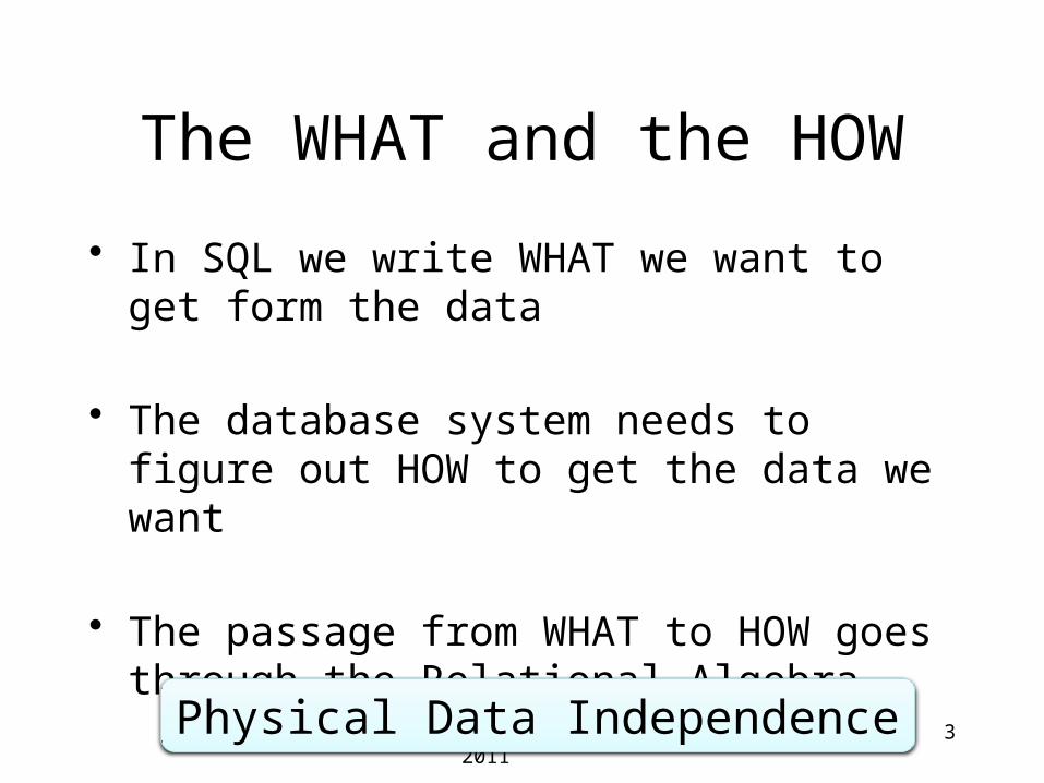
The WHAT and the HOW
• In SQL we write WHAT we want to get form the data
• The database system needs to figure out HOW to get the data we want
• The passage from WHAT to HOW goes through the Relational Algebra
3Dan Suciu -- 544, Winter 2011 Physical Data Independence
4
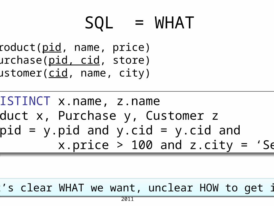
SQL = WHAT
SELECT DISTINCT x.name, z.nameFROM Product x, Purchase y, Customer zWHERE x.pid = y.pid and y.cid = y.cid and x.price > 100 and z.city = ‘Seattle’
Dan Suciu -- 544, Winter 2011 It’s clear WHAT we want, unclear HOW to get it
Product(pid, name, price)Purchase(pid, cid, store)Customer(cid, name, city)

5
Relational Algebra = HOW
Product Purchase
pid=pid
price>100 and city=‘Seattle’
x.name,z.name
δProduct(pid, name, price)Purchase(pid, cid, store)Customer(cid, name, city)
cid=cid
Customer
Π
σ
T1(pid,name,price,pid,cid,store)
T2( . . . .)
T4(name,name)
Final answer
T3(. . . )
Temporary tablesT1, T2, . . .
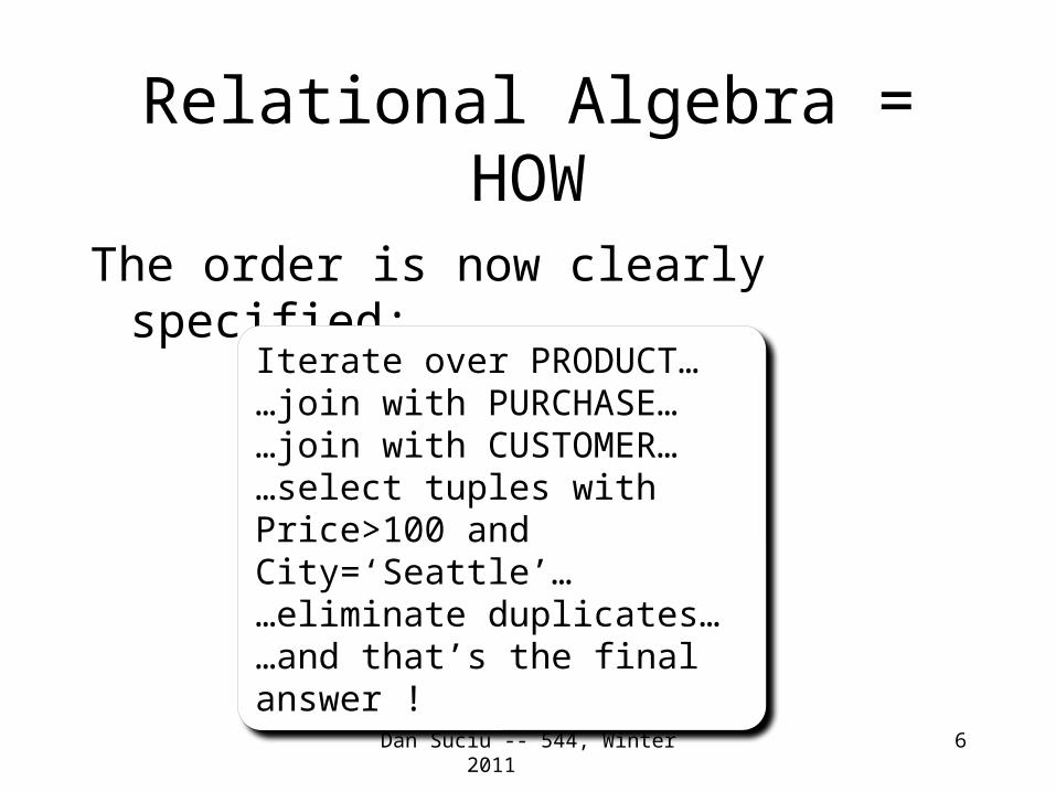
Relational Algebra = HOW
The order is now clearly specified:
6Dan Suciu -- 544, Winter 2011
Iterate over PRODUCT……join with PURCHASE……join with CUSTOMER……select tuples with Price>100 and City=‘Seattle’……eliminate duplicates……and that’s the final answer !

Sets v.s. Bags
• Sets: {a,b,c}, {a,d,e,f}, { }, . . .• Bags: {a, a, b, c}, {b, b, b, b, b}, . . .
Relational Algebra has two semantics:• Set semantics• Bag semantics
7Dan Suciu -- 544, Winter 2011

Dan Suciu -- 544, Winter 2011
Extended Algebra Operators
• Union , intersection , difference - • Selection s• Projection Π• Join ⨝• Rename • Duplicate elimination d• Grouping and aggregation g• Sorting t
8

9
Relational Algebra (1/3)The Basic Five operators:• Union: • Difference: -• Selection: s• Projection: P • Join: ⨝
Dan Suciu -- 544, Winter 2011

10
Relational Algebra (2/3)
Derived or auxiliary operators:• Renaming: ρ • Intersection, complement• Variations of joins–natural, equi-join, theta join,
semi-join, cartesian product
Dan Suciu -- 544, Winter 2011
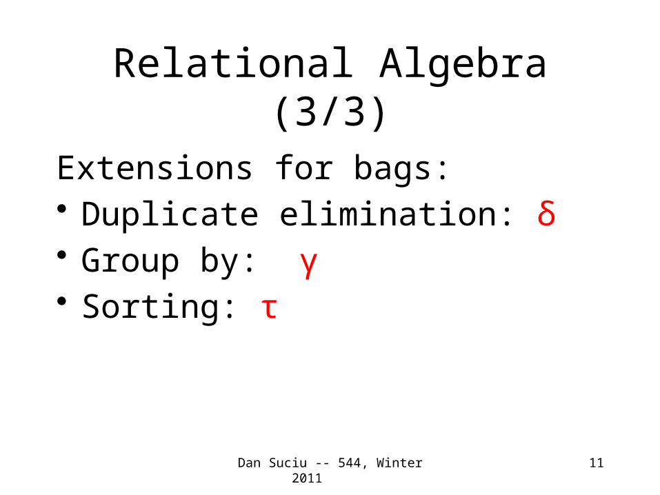
Relational Algebra (3/3)
Extensions for bags:• Duplicate elimination: δ• Group by: γ• Sorting: τ
11Dan Suciu -- 544, Winter 2011

Union and Difference
Dan Suciu -- 544, Winter 2011 12
What do they mean over bags ?
R1 R2R1 – R2
13
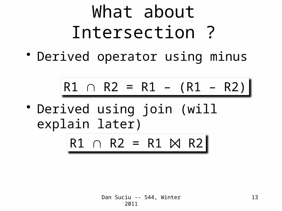
What about Intersection ?
• Derived operator using minus
• Derived using join (will explain later)
Dan Suciu -- 544, Winter 2011
R1 R2 = R1 – (R1 – R2)
R1 R2 = R1 R2⨝

14
Selection• Returns all tuples which satisfy a
condition
• Examples– sSalary > 40000 (Employee)– sname = “Smith” (Employee)
• The condition c can be =, <, , >, , <>Dan Suciu -- 544, Winter 2011
sc(R)

15
sSalary > 40000 (Employee)
SSN Name Salary
1234545 John 200000
5423341 Smith 600000
4352342 Fred 500000
SSN Name Salary
5423341 Smith 600000
4352342 Fred 500000
Dan Suciu -- 544, Winter 2011
Employee

16
Projection• Eliminates columns
• Example: project social-security number and names:– P SSN, Name (Employee)
– Answer(SSN, Name)
Semantics differs over set or over bags
Dan Suciu -- 544, Winter 2011
P A1,…,An (R)

17
P Name,Salary (Employee)
SSN Name Salary
1234545 John 20000
5423341 John 60000
4352342 John 20000
Name Salary
John 20000
John 60000
John 20000
Dan Suciu -- 544, Winter 2011
Employee
Name Salary
John 20000
John 60000
Bag semantics Set semantics
Which is more efficient to implement ?
18
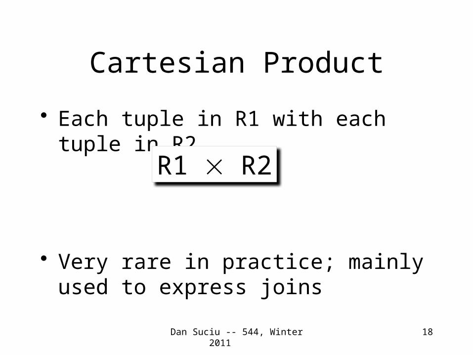
Cartesian Product
• Each tuple in R1 with each tuple in R2
• Very rare in practice; mainly used to express joins
Dan Suciu -- 544, Winter 2011
R1 R2
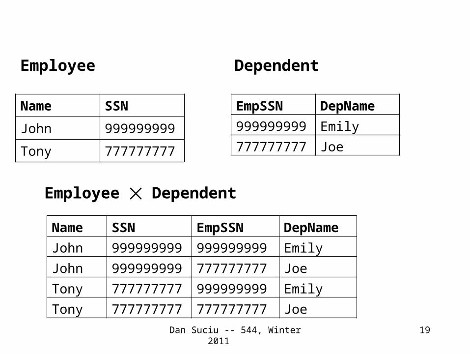
19Dan Suciu -- 544, Winter 2011
Name SSN
John 999999999
Tony 777777777
Employee
EmpSSN DepName
999999999 Emily
777777777 Joe
Dependent
Employee ✕ Dependent
Name SSN EmpSSN DepName
John 999999999 999999999 Emily
John 999999999 777777777 Joe
Tony 777777777 999999999 Emily
Tony 777777777 777777777 Joe
20
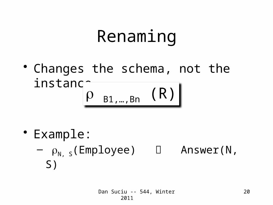
Renaming
• Changes the schema, not the instance
• Example:– rN, S(Employee) Answer(N, S)
Dan Suciu -- 544, Winter 2011
r B1,…,Bn (R)

21
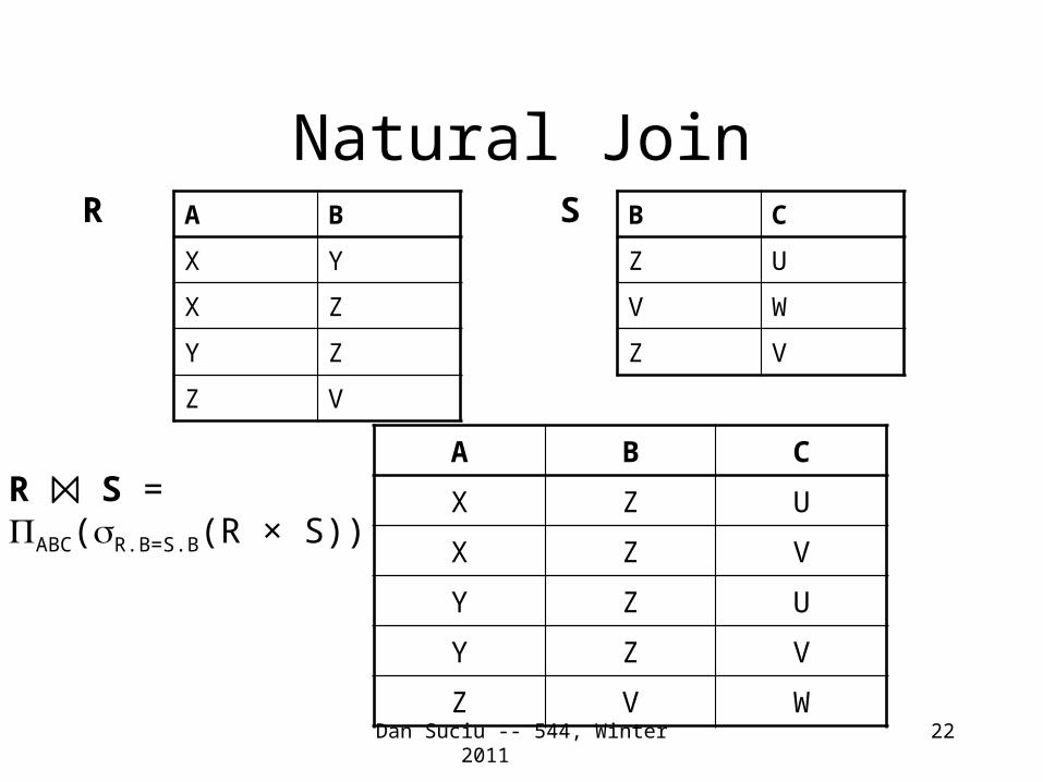
Natural Join
• Meaning: R1⨝ R2 = PA(s(R1 × R2))
• Where:– The selection s checks equality of all
common attributes– The projection eliminates the duplicate
common attributes
Dan Suciu -- 544, Winter 2011
R1 ⨝ R2
Natural Join
Dan Suciu -- 544, Winter 2011 22
A B
X Y
X Z
Y Z
Z V
B C
Z U
V W
Z V
A B C
X Z U
X Z V
Y Z U
Y Z V
Z V W
R S
R ⨝ S =PABC(sR.B=S.B(R × S))

23
Natural Join
• Given the schemas R(A, B, C, D), S(A, C, E), what is the schema of R S ?⨝
• Given R(A, B, C), S(D, E), what is R ⨝S ?
• Given R(A, B), S(A, B), what is R S ?⨝
Dan Suciu -- 544, Winter 2011

24
Theta Join
• A join that involves a predicate
• Here q can be any condition
Dan Suciu -- 544, Winter 2011
R1 ⨝q R2 = s q (R1 R2)

25
Eq-join
• A theta join where q is an equality
• This is by far the most used variant of join in practice
Dan Suciu -- 544, Winter 2011
R1 ⨝A=B R2 = sA=B (R1 R2)

So Which Join Is It ?
• When we write R S we usually mean ⨝an eq-join, but we often omit the equality predicate when it is clear from the context
26Dan Suciu -- 544, Winter 2011

27
Semijoin
• Where A1, …, An are the attributes in R
Dan Suciu -- 544, Winter 2011
R ⋉C S = P A1,…,An (R ⨝C S)
Formally, R ⋉C S means this: retain from R only thosetuples that have some matching tuple in S• Duplicates in R are preserved• Duplicates in S don’t matter

Semijoins in Distributed Databases
28
SSN Name Stuff
. . . . . . . . . .
EmpSSN DepName Age Stuff
. . . . . . . . . . . . .
EmployeeDependent
network
Employee ⨝SSN=EmpSSN ( s age>71 (Dependent))
Task: compute the query with minimum amount of data transfer
Assumptions: Very few Employees have dependents.Very few dependents have age > 71.“Stuff” is big.

Semijoins in Distributed Databases
29
SSN Name Stuff
. . . . . . . . . .
EmpSSN DepName Age Stuff
. . . . . . . . . . . . .
EmployeeDependent
network
Employee ⨝SSN=EmpSSN ( s age>71 (Dependent))
T(SSN) = P SSN s age>71 (Dependents)
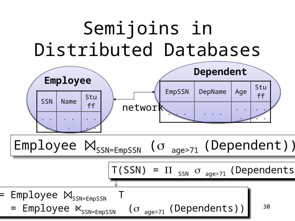
Semijoins in Distributed Databases
30
SSN Name Stuff
. . . . . . . . . .
EmpSSN DepName Age Stuff
. . . . . . . . . . . . .
EmployeeDependent
network
R = Employee ⨝SSN=EmpSSN T = Employee ⋉SSN=EmpSSN ( s age>71 (Dependents))
T(SSN) = P SSN s age>71 (Dependents)
Employee ⨝SSN=EmpSSN ( s age>71 (Dependent))

Semijoins in Distributed Databases
31
SSN Name Stuff
. . . . . . . . . .
EmpSSN DepName Age Stuff
. . . . . . . . . . . . .
EmployeeDependent
network
T(SSN) = P SSN s age>71 (Dependents)
R = Employee ⋉SSN=EmpSSN T
Answer = R ⨝SSN=EmpSSN Dependents
Employee ⨝SSN=EmpSSN ( s age>71 (Dependent))

32
Joins R US
• The join operation in all its variants (eq-join, natural join, semi-join, outer-join) is at the heart of relational database systems
• WHY ?
Dan Suciu -- 544, Winter 2011

33
Operators on Bags
• Duplicate elimination dd(R) = select distinct * from R
• Grouping ggA,sum(B) (R) = select A,sum(B) from R group by A
• Sorting t
Dan Suciu -- 544, Winter 2011
34
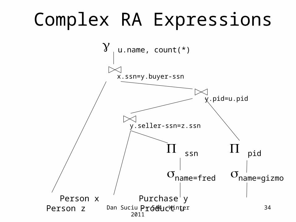
Complex RA Expressions
Person x Purchase y Person z Product u
sname=fred sname=gizmo
P pidP ssn
y.seller-ssn=z.ssn
y.pid=u.pid
x.ssn=y.buyer-ssn
g u.name, count(*)
Dan Suciu -- 544, Winter 2011

RA = Dataflow Program
• Several operations, plus strictly specified order
• In RDBMS the dataflow graph is always a tree
• Novel applications (s.a. PIG), dataflow graph may be a DAG
35Dan Suciu -- 544, Winter 2011

36
Limitations of RA
• Cannot compute “transitive closure”
• Find all direct and indirect relatives of Fred• Cannot express in RA !!! Need to write Java program• Remember the Bacon number ? Needs TC too !
Name1 Name2 Relationship
Fred Mary Father
Mary Joe Cousin
Mary Bill Spouse
Nancy Lou Sister
Dan Suciu -- 544, Winter 2011

Steps of the Query Processor
Parse & Rewrite Query
Select Logical Plan
Select Physical Plan
Query Execution
Disk
SQL query
Queryoptimization
Logicalplan
Physicalplan
37
Dan Suciu -- 544, Winter 2011
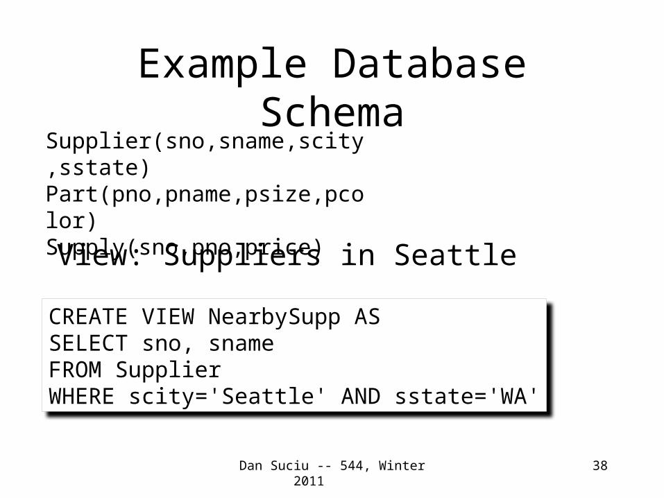
Example Database Schema
View: Suppliers in Seattle
38
CREATE VIEW NearbySupp ASSELECT sno, snameFROM SupplierWHERE scity='Seattle' AND sstate='WA'
Supplier(sno,sname,scity,sstate)Part(pno,pname,psize,pcolor)Supply(sno,pno,price)

Dan Suciu -- 544, Winter 2011
Example Query
Find the names of all suppliers in Seattle
who supply part number 2
39
SELECT sname FROM NearbySuppWHERE sno IN ( SELECT sno FROM Supplies WHERE pno = 2 )
Dan Suciu -- 544, Winter 2011
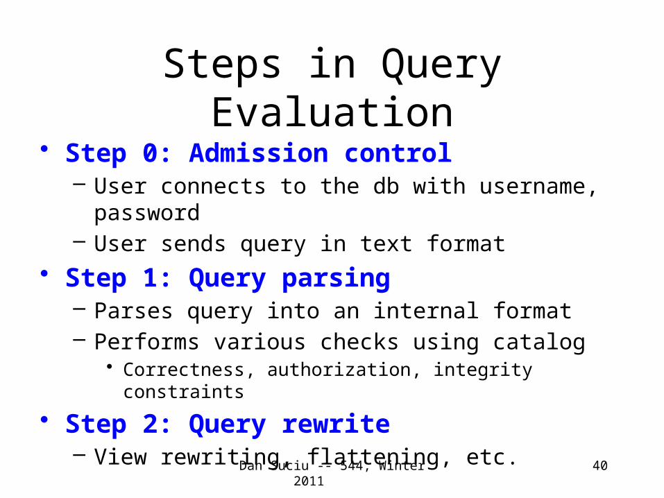
Steps in Query Evaluation• Step 0: Admission control
– User connects to the db with username, password– User sends query in text format
• Step 1: Query parsing– Parses query into an internal format– Performs various checks using catalog
• Correctness, authorization, integrity constraints
• Step 2: Query rewrite– View rewriting, flattening, etc.
40

Dan Suciu -- 544, Winter 2011
Rewritten Version of Our Query
Original query:
Rewritten query:
41
SELECT snameFROM NearbySuppWHERE sno IN ( SELECT sno FROM Supplies WHERE pno = 2 )
SELECT S.snameFROM Supplier S, Supplies UWHERE S.scity='Seattle' AND S.sstate='WA’AND S.sno = U.snoAND U.pno = 2;

Dan Suciu -- 544, Winter 2011
Continue with Query Evaluation
• Step 3: Query optimization– Find an efficient query plan for executing the query
• A query plan is– Logical query plan: an extended relational algebra tree – Physical query plan: with additional annotations at each
node• Access method to use for each relation• Implementation to use for each relational operator
42

Dan Suciu -- 544, Winter 2011
Extended Algebra Operators
• Union , intersection , difference - • Selection s• Projection • Join ⨝• Duplicate elimination d• Grouping and aggregation g• Sorting t• Rename
43
Dan Suciu -- 544, Winter 2011
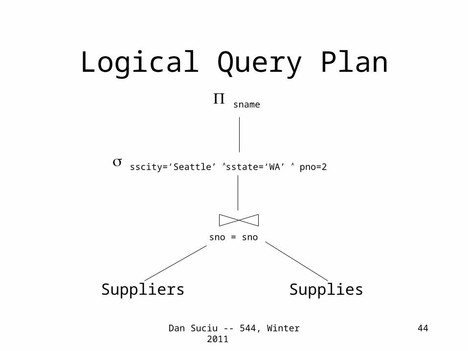
Logical Query Plan
Suppliers Supplies
sno = sno
sscity=‘Seattle’ sstate=‘WA’ pno=2
Πsname
44
Dan Suciu -- 544, Winter 2011
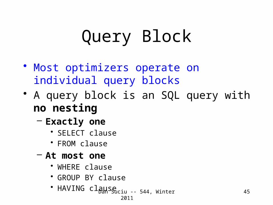
Query Block
• Most optimizers operate on individual query blocks
• A query block is an SQL query with no nesting– Exactly one
• SELECT clause• FROM clause
– At most one• WHERE clause• GROUP BY clause• HAVING clause
45
Dan Suciu -- 544, Winter 2011
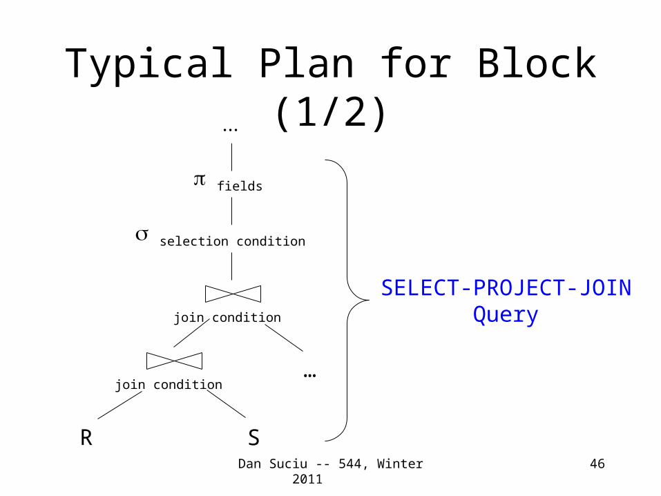
Typical Plan for Block (1/2)
R S
join condition
selection condition
fields
join condition
…
SELECT-PROJECT-JOINQuery
46
Dan Suciu -- 544, Winter 2011
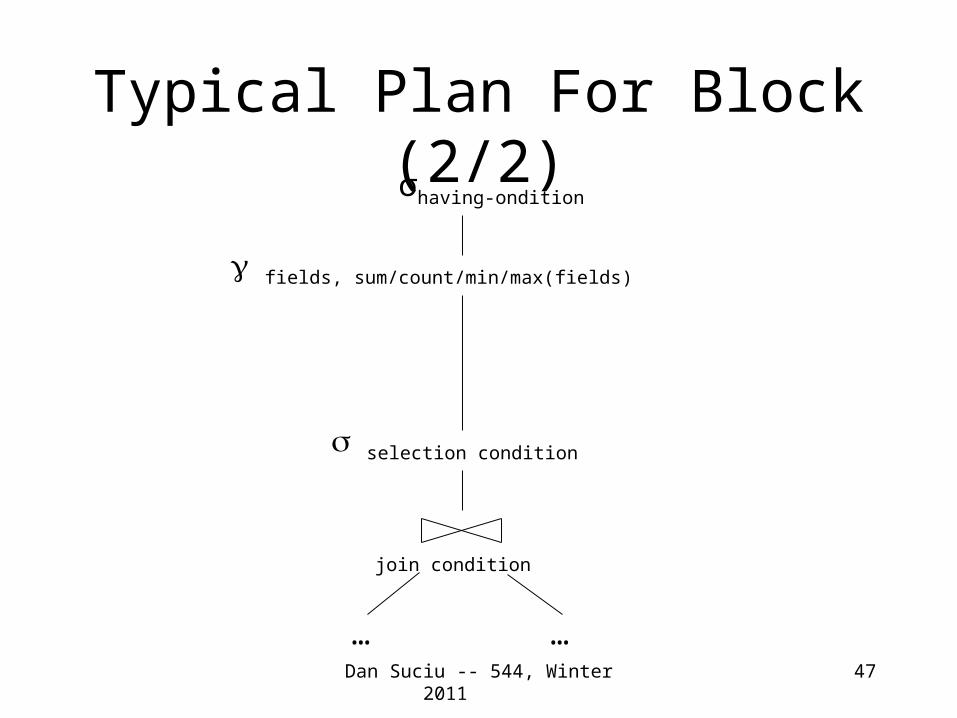
Typical Plan For Block (2/2)
fields, sum/count/min/max(fields)
σhaving-ondition
selection condition
join condition
… …47

Dan Suciu -- 544, Winter 2011
How about Subqueries?
SELECT Q.snoFROM Supplier QWHERE Q.sstate = ‘WA’ and not exists SELECT * FROM Supply P WHERE P.sno = Q.sno and P.price > 100
48
Supplier(sno,sname,scity,sstate)Part(pno,pname,psize,pcolor)Supply(sno,pno,price)

Dan Suciu -- 544, Winter 2011
How about Subqueries?
SELECT Q.snoFROM Supplier QWHERE Q.sstate = ‘WA’ and not exists SELECT * FROM Supply P WHERE P.sno = Q.sno and P.price > 100
49
Correlation !
Supplier(sno,sname,scity,sstate)Part(pno,pname,psize,pcolor)Supply(sno,pno,price)

Dan Suciu -- 544, Winter 2011
How about Subqueries?
SELECT Q.snoFROM Supplier QWHERE Q.sstate = ‘WA’ and not exists SELECT * FROM Supply P WHERE P.sno = Q.sno and P.price > 100
50
De-Correlation
SELECT Q.snoFROM Supplier QWHERE Q.sstate = ‘WA’ and Q.sno not in SELECT P.sno FROM Supply P WHERE P.price > 100
Supplier(sno,sname,scity,sstate)Part(pno,pname,psize,pcolor)Supply(sno,pno,price)
Dan Suciu -- 544, Winter 2011
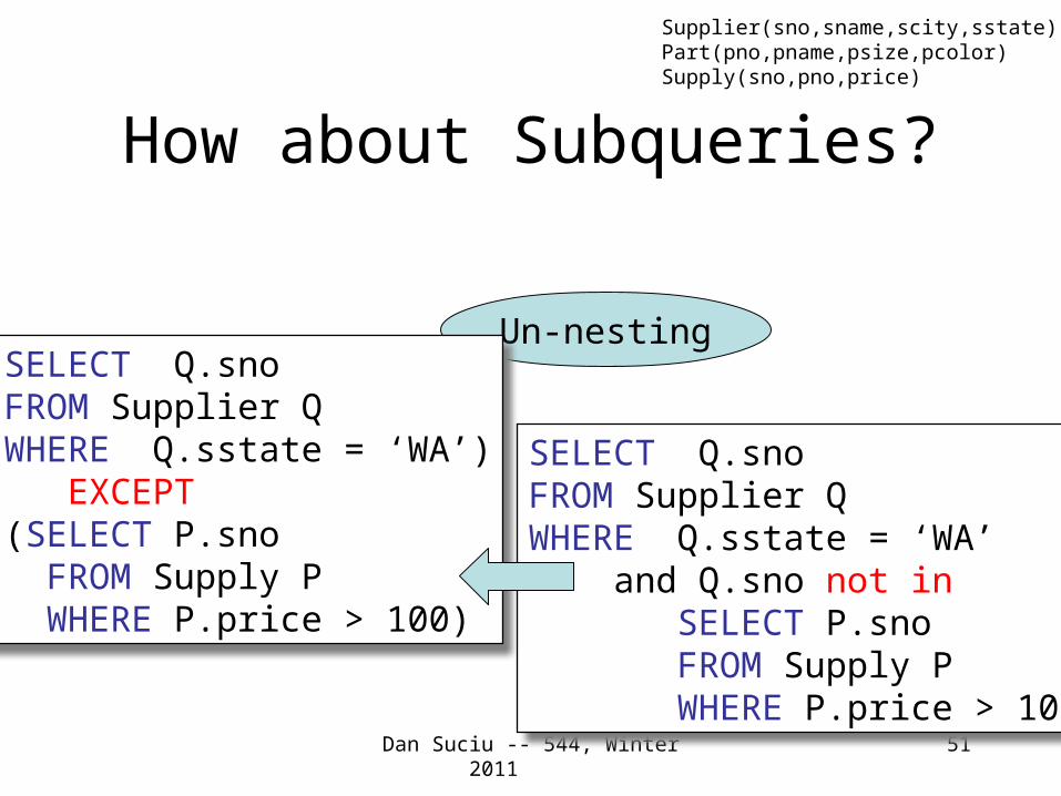
How about Subqueries?
51
Un-nesting
SELECT Q.snoFROM Supplier QWHERE Q.sstate = ‘WA’ and Q.sno not in SELECT P.sno FROM Supply P WHERE P.price > 100
(SELECT Q.sno FROM Supplier Q WHERE Q.sstate = ‘WA’) EXCEPT (SELECT P.sno FROM Supply P WHERE P.price > 100)
Supplier(sno,sname,scity,sstate)Part(pno,pname,psize,pcolor)Supply(sno,pno,price)
Dan Suciu -- 544, Winter 2011
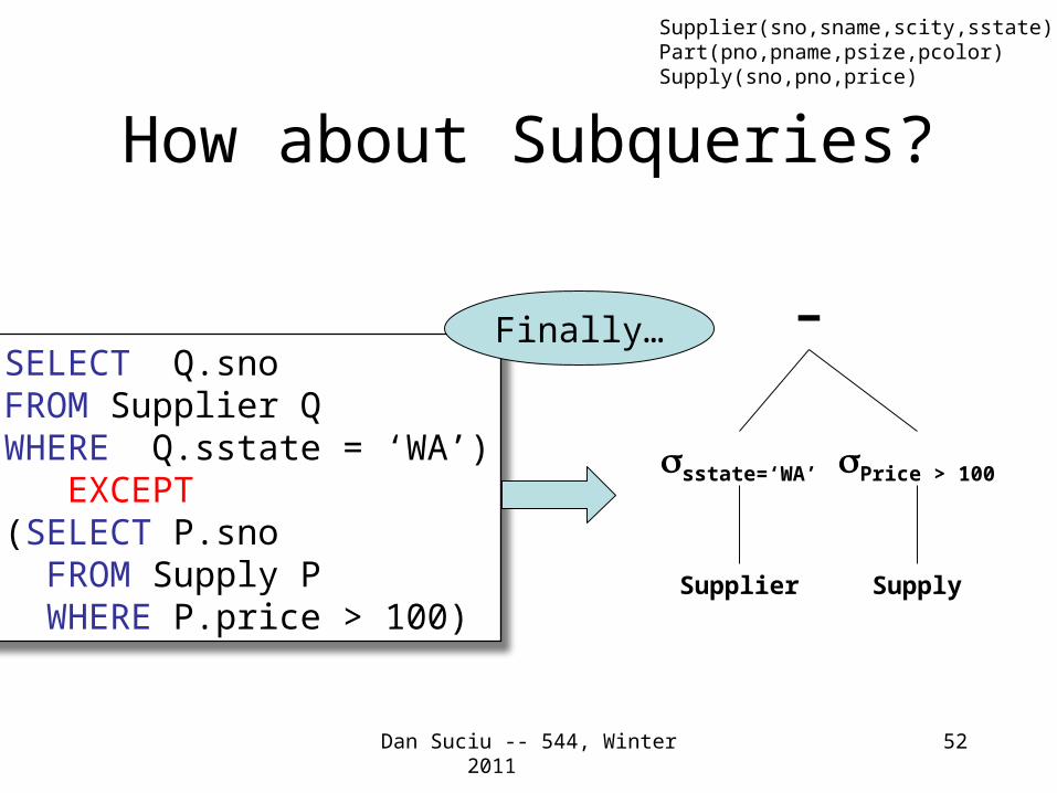
How about Subqueries?
Supply
sstate=‘WA’
Supplier
Price > 100
52
(SELECT Q.sno FROM Supplier Q WHERE Q.sstate = ‘WA’) EXCEPT (SELECT P.sno FROM Supply P WHERE P.price > 100)
−
Supplier(sno,sname,scity,sstate)Part(pno,pname,psize,pcolor)Supply(sno,pno,price)
Finally…
Dan Suciu -- 544, Winter 2011
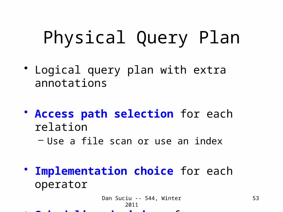
Physical Query Plan
• Logical query plan with extra annotations
• Access path selection for each relation– Use a file scan or use an index
• Implementation choice for each operator
• Scheduling decisions for operators
53

Dan Suciu -- 544, Winter 2011
Physical Query Plan
Suppliers Supplies
sno = sno
sscity=‘Seattle’ sstate=‘WA’ pno=2
sname
(File scan) (File scan)
(Nested loop)
(On the fly)
(On the fly)
54
Supplier(sno,sname,scity,sstate)Part(pno,pname,psize,pcolor)Supply(sno,pno,price)

Dan Suciu -- 544, Winter 2011
Final Step in Query Processing
• Step 4: Query execution– How to synchronize operators?– How to pass data between operators?
• What techniques are possible?– One thread per query– Iterator interface – Pipelined execution– Intermediate result materialization
55
Dan Suciu -- 544, Winter 2011
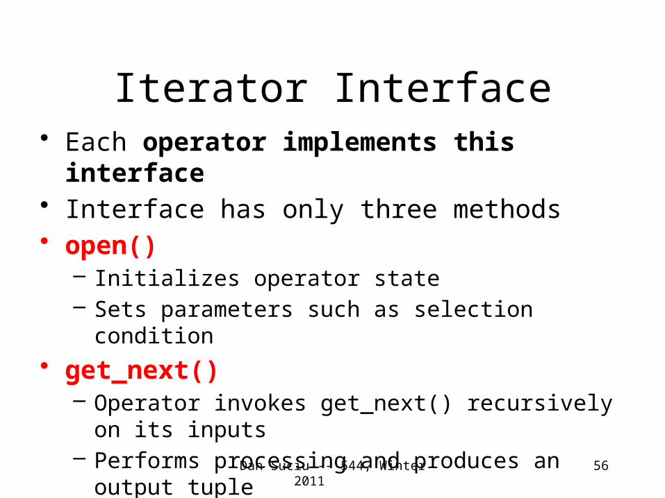
Iterator Interface• Each operator implements this interface• Interface has only three methods• open()
– Initializes operator state– Sets parameters such as selection condition
• get_next()– Operator invokes get_next() recursively on its inputs– Performs processing and produces an output tuple
• close(): cleans-up state
56

Dan Suciu -- 544, Winter 2011
Pipelined Execution
Suppliers Supplies
sno = sno
sscity=‘Seattle’ sstate=‘WA’ pno=2
sname
(File scan) (File scan)
(Nested loop)
(On the fly)
(On the fly)
57
Supplier(sno,sname,scity,sstate)Part(pno,pname,psize,pcolor)Supply(sno,pno,price)

Dan Suciu -- 544, Winter 2011
Pipelined Execution
• Applies parent operator to tuples directly as they are produced by child operators
• Benefits– No operator synchronization issues– Saves cost of writing intermediate data to disk– Saves cost of reading intermediate data from disk– Good resource utilizations on single processor
• This approach is used whenever possible
58

Dan Suciu -- 544, Winter 2011
Suppliers Supplies
sno = sno
sscity=‘Seattle’ sstate=‘WA’
sname
(File scan) (File scan)
(Sort-merge join)
(Scan: write to T2)
(On the fly)
pno=2
(Scan: write to T1)
Intermediate Tuple Materialization
59
Supplier(sno,sname,scity,sstate)Part(pno,pname,psize,pcolor)Supply(sno,pno,price)

Intermediate Tuple Materialization
• Writes the results of an operator to an intermediate table on disk
• No direct benefit but• Necessary data is larger than main memory• Necessary when operator needs to examine
the same tuples multiple times
Dan Suciu -- 544, Winter 2011 60

61
Physical Operators
Each of the logical operators may have one or more implementations = physical operators
Will discuss several basic physical operators, with a focus on join
Dan Suciu -- 544, Winter 2011

62
Question in Class
Logical operator:
Supply(sno,pno,price) ⨝pno=pno Part(pno,pname,psize,pcolor)
Propose three physical operators for the join, assuming the tables are in main memory:
1. 2. 3.
Dan Suciu -- 544, Winter 2011
Supplier(sno,sname,scity,sstate)Part(pno,pname,psize,pcolor)Supply(sno,pno,price)

63
Question in Class
Logical operator:
Supply(sno,pno,price) ⨝pno=pno Part(pno,pname,psize,pcolor)
Propose three physical operators for the join, assuming the tables are in main memory:
1. Nested Loop Join2. Merge join3. Hash join
Dan Suciu -- 544, Winter 2011
Supplier(sno,sname,scity,sstate)Part(pno,pname,psize,pcolor)Supply(sno,pno,price)

1. Nested Loop Join
64
for S in Supply do {
for P in Part do {
if (S.pno == P.pno) output(S,P);
}
}
Supplier(sno,sname,scity,sstate)Part(pno,pname,psize,pcolor)Supply(sno,pno,price)
Supply = outer relationPart = inner relationNote: sometimes terminology is switched
Would it be more efficient tochoose Part=inner, Supply=outer ?What if we had an index on Part.pno ?
Dan Suciu -- 544, Winter 2011
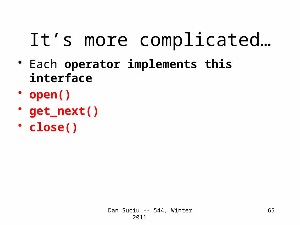
It’s more complicated…• Each operator implements this interface• open()• get_next()• close()
65

Main Memory Nested Loop Join Revisited
66
open ( ) { Supply.open( ); Part.open( ); S = Supply.get_next( ); }
Supplier(sno,sname,scity,sstate)Part(pno,pname,psize,pcolor)Supply(sno,pno,price)
get_next( ) { repeat { P= Part.get_next( ); if (P== NULL) { Part.close(); S= Supply.get_next( ); if (S== NULL) return NULL; Part.open( ); P= Part.get_next( ); } until (S.pno == P.pno); return (S, P)}
close ( ) { Supply.close ( ); Part.close ( ); }
ALL operators need to be implemented this way !

67
BRIEF Review of Hash Tables
0
1
2
3
4
5
6
7
8
9
Separate chaining:
h(x) = x mod 10
A (naïve) hash function:
503
103
76 666
48
503
Duplicates OK
WHY ??
Operations:
find(103) = ??
insert(488) = ??

68
BRIEF Review of Hash Tables
• insert(k, v) = inserts a key k with value v
• Many values for one key– Hence, duplicate k’s are OK
• find(k) = returns the list of all values v associated to the key k
Dan Suciu -- 544, Winter 2011

2. Hash Join (main memory)
69
for S in Supply do insert(S.pno, S);
for P in Part do {
LS = find(P.pno);
for S in LS do { output(S, P); }
}
Supplier(sno,sname,scity,sstate)Part(pno,pname,psize,pcolor)Supply(sno,pno,price)
Recall: need to rewrite as open, get_next, close
Buildphase
Probing
Supply=outer Part=inner
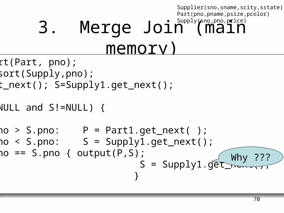
3. Merge Join (main memory)
70
Part1 = sort(Part, pno);Supply1 = sort(Supply,pno);P=Part1.get_next(); S=Supply1.get_next();
While (P!=NULL and S!=NULL) { case: P.pno > S.pno: P = Part1.get_next( ); P.pno < S.pno: S = Supply1.get_next(); P.pno == S.pno { output(P,S); S = Supply1.get_next(); }}
Supplier(sno,sname,scity,sstate)Part(pno,pname,psize,pcolor)Supply(sno,pno,price)
Why ???

71
Main Memory Group By
Grouping:
Product(name, department, quantity)
gdepartment, sum(quantity) (Product) Answer(department, sum)
Main memory hash table
Question: How ?
Dan Suciu -- 544, Winter 2011
72
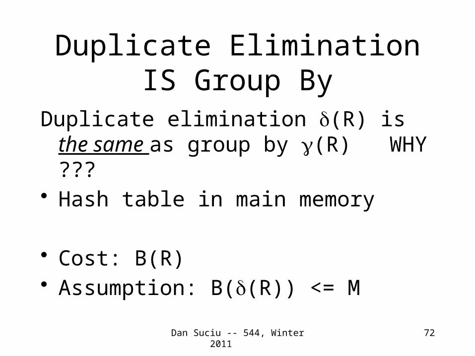
Duplicate Elimination IS Group By
Duplicate elimination d(R) is the same as group by g(R) WHY ???
• Hash table in main memory
• Cost: B(R)• Assumption: B(d(R)) <= M
Dan Suciu -- 544, Winter 2011

73
Selections, Projections
• Selection = easy, check condition on each tuple at a time
• Projection = easy (assuming no duplicate elimination), remove extraneous attributes from each tuple
Dan Suciu -- 544, Winter 2011
Dan Suciu -- 544, Winter 2011
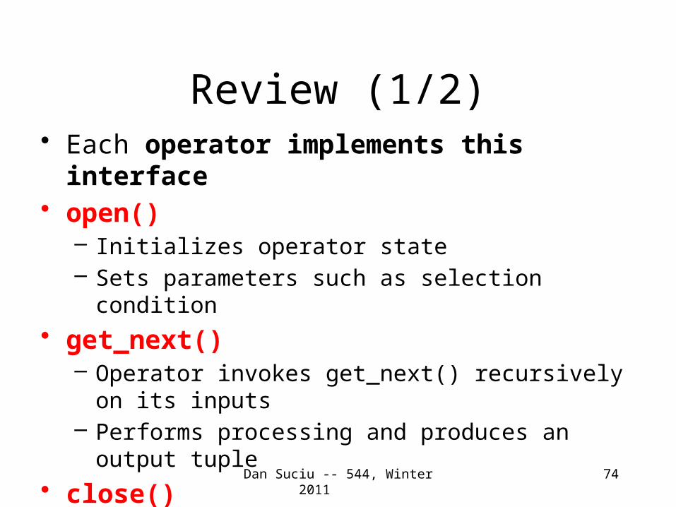
Review (1/2)• Each operator implements this interface• open()
– Initializes operator state– Sets parameters such as selection condition
• get_next()– Operator invokes get_next() recursively on its inputs– Performs processing and produces an output tuple
• close()– Cleans-up state
74

75
Review (2/2)
• Three algorithms for main memory join:– Nested loop join– Hash join– Merge join
• Algorithms for selection, projection, group-by
Dan Suciu -- 544, Winter 2011
If |R| = m and |S| = n, what is the asymptoticcomplexity for computing R S ?⋈
76
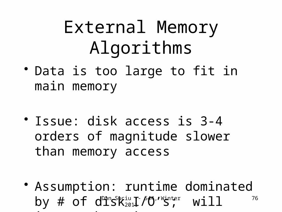
External Memory Algorithms
• Data is too large to fit in main memory
• Issue: disk access is 3-4 orders of magnitude slower than memory access
• Assumption: runtime dominated by # of disk I/O’s; will ignore the main memory part of the runtime
Dan Suciu -- 544, Winter 2011
77
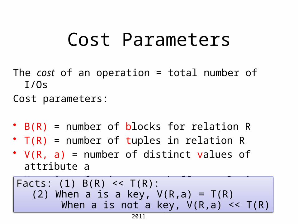
Cost Parameters
The cost of an operation = total number of I/Os
Cost parameters:
• B(R) = number of blocks for relation R• T(R) = number of tuples in relation R• V(R, a) = number of distinct values of attribute a• M = size of main memory buffer pool, in blocks
Dan Suciu -- 544, Winter 2011
Facts: (1) B(R) << T(R):(2) When a is a key, V(R,a) = T(R) When a is not a key, V(R,a) << T(R)
78
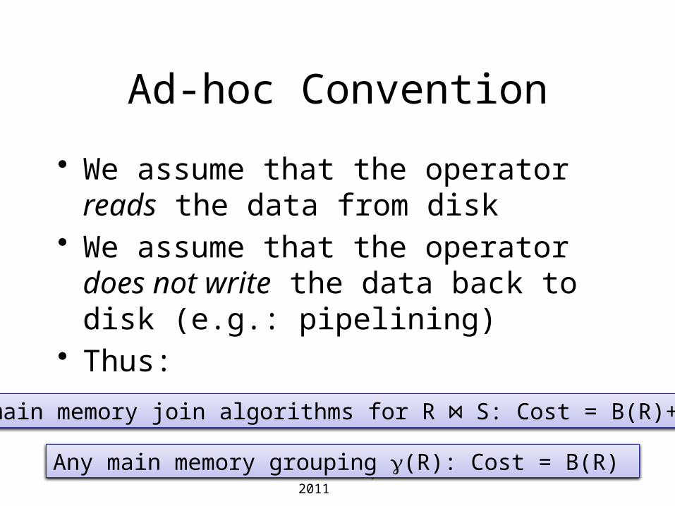
Ad-hoc Convention
• We assume that the operator reads the data from disk
• We assume that the operator does not write the data back to disk (e.g.: pipelining)
• Thus:
Dan Suciu -- 544, Winter 2011
Any main memory join algorithms for R S: Cost = B(R)+B(S) ⋈
Any main memory grouping g(R): Cost = B(R)

79
Sequential Scan of a Table R
• When R is clustered – Blocks consists only of records from this table– B(R) << T(R)– Cost = B(R)
• When R is unclustered – Its records are placed on blocks with other tables– B(R) T(R)– Cost = T(R)
Dan Suciu -- 544, Winter 2011
80
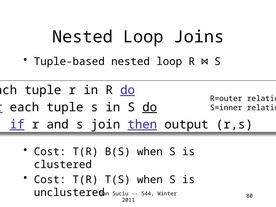
Nested Loop Joins• Tuple-based nested loop R ⋈ S
• Cost: T(R) B(S) when S is clustered• Cost: T(R) T(S) when S is unclustered
for each tuple r in R do
for each tuple s in S do
if r and s join then output (r,s)
Dan Suciu -- 544, Winter 2011
R=outer relationS=inner relation

81
Examples
M = 4; R, S are clustered• Example 1:
– B(R) = 1000, T(R) = 10000– B(S) = 2, T(S) = 20– Cost = ?
• Example 2:– B(R) = 1000, T(R) = 10000– B(S) = 4, T(S) = 40– Cost = ?
Dan Suciu -- 544, Winter 2011
Can you do better ?

82
Block-Based Nested-loop Join
for each (M-2) blocks bs of S do
for each block br of R do
for each tuple s in bs
for each tuple r in br do
if “r and s join” then output(r,s)
Dan Suciu -- 544, Winter 2011
Terminology alert: book calls S the inner relation
Why not M ?

83
Block Nested-loop Join
. . .
. . .
R & SHash table for block of S
(M-2 pages)
Input buffer for R Output buffer
. . .
Join Result
Dan Suciu -- 544, Winter 2011

84
ExamplesM = 4; R, S are clustered• Example 1:
– B(R) = 1000, T(R) = 10000– B(S) = 2, T(S) = 20– Cost = B(S) + B(R) = 1002
• Example 2:– B(R) = 1000, T(R) = 10000– B(S) = 4, T(S) = 40– Cost = B(S) + 2B(R) = 2004
Dan Suciu -- 544, Winter 2011
Note: T(R) andT(S) are irrelevanthere.

85
Cost of Block Nested-loop Join
• Read S once: cost B(S)• Outer loop runs B(S)/(M-2) times, and
each time need to read R: costs B(S)B(R)/(M-2)
Dan Suciu -- 544, Winter 2011
Cost = B(S) + B(S)B(R)/(M-2)

Index Based Selection
Dan Suciu -- 544, Winter 2011 86
SELET *
FROM Movie
WHERE id = ‘12345’
Recall IMDB; assume indexes on Movie.id, Movie.year
SELET *
FROM Movie
WHERE year = ‘1995’
B(Movie) = 10kT(Movie) = 1M
What is your estimateof the I/O cost ?

87
Index Based Selection
Selection on equality: sa=v(R)
• Clustered index on a: cost B(R)/V(R,a)
• Unclustered index : cost T(R)/V(R,a)
Dan Suciu -- 544, Winter 2011

88
Index Based Selection
• Example:
• Table scan (assuming R is clustered):– B(R) = 10k I/Os
• Index based selection:– If index is clustered: B(R)/V(R,a) = 100 I/Os– If index is unclustered: T(R)/V(R,a) = 10000 I/Os
B(R) = 10kT(R) = 1MV(R, a) = 100
cost of sa=v(R) = ?
Dan Suciu -- 544, Winter 2011
Rule of thumb: don’t build unclustered indexes when V(R,a) is small !

89
Index Based Join
• R S⨝• Assume S has an index on the join
attribute
for each tuple r in R do
lookup the tuple(s) s in S using the indexoutput (r,s)
Dan Suciu -- 544, Winter 2011

90
Index Based Join
Cost (Assuming R is clustered):
• If index is clustered: B(R) + T(R)B(S)/V(S,a)• If unclustered: B(R) + T(R)T(S)/V(S,a)
Dan Suciu -- 544, Winter 2011

91
Operations on Very Large Tables
• Compute R S when each is larger ⋈than main memory
• Two methods:– Partitioned hash join (many variants)– Merge-join
• Similar for groupingDan Suciu -- 544, Winter 2011
92
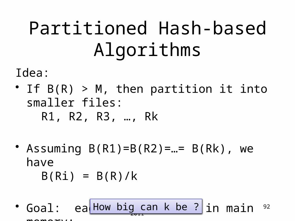
Partitioned Hash-based Algorithms
Idea:• If B(R) > M, then partition it into smaller files:
R1, R2, R3, …, Rk
• Assuming B(R1)=B(R2)=…= B(Rk), we haveB(Ri) = B(R)/k
• Goal: each Ri should fit in main memory: B(Ri) ≤ M
Dan Suciu -- 544, Winter 2011 How big can k be ?
93
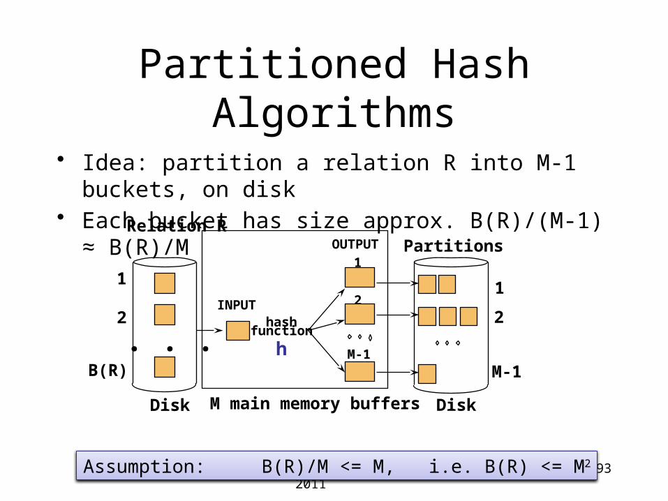
Partitioned Hash Algorithms
• Idea: partition a relation R into M-1 buckets, on disk• Each bucket has size approx. B(R)/(M-1) ≈ B(R)/M
M main memory buffers DiskDisk
Relation ROUTPUT
2INPUT
1
hashfunction
h M-1
Partitions
1
2
M-1
. . .
1
2
B(R)
Dan Suciu -- 544, Winter 2011 Assumption: B(R)/M <= M, i.e. B(R) <= M2
94
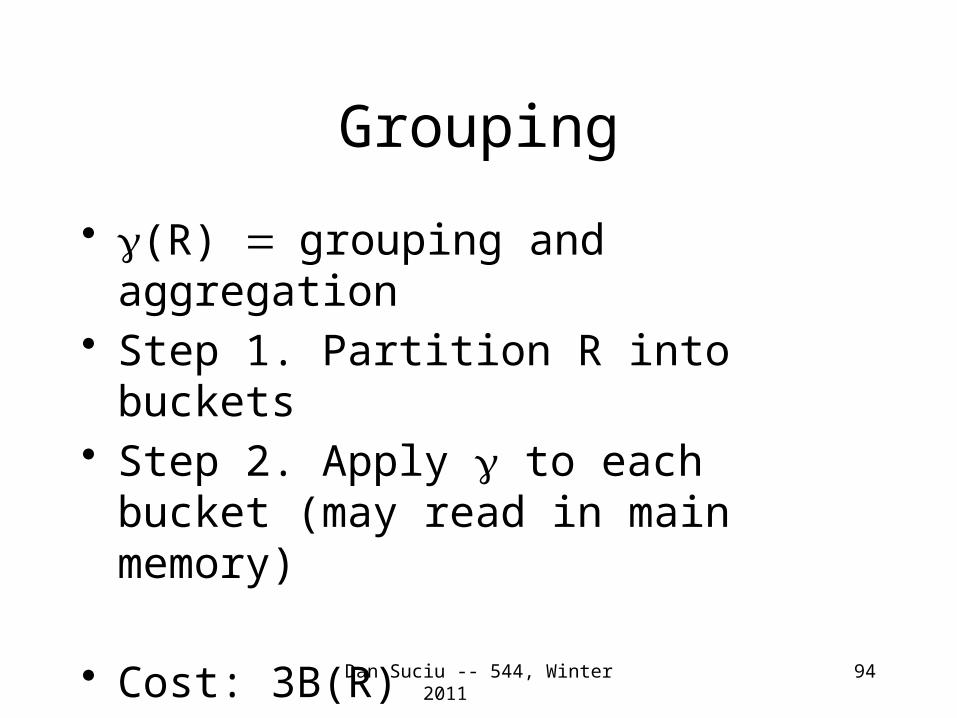
Grouping
• g(R) = grouping and aggregation• Step 1. Partition R into buckets• Step 2. Apply g to each bucket (may
read in main memory)
• Cost: 3B(R)• Assumption: B(R) <= M2
Dan Suciu -- 544, Winter 2011

95
Partitioned Hash JoinGRACE Join
R ⨝ S• Step 1:
– Hash S into M buckets– send all buckets to disk
• Step 2– Hash R into M buckets– Send all buckets to disk
• Step 3– Join every pair of buckets
Dan Suciu -- 544, Winter 2011

96
Grace-Join• Partition both relations
using hash fn h: R tuples in partition i will only match S tuples in partition i.
Read in a partition of R, hash it using h2 (<> h!). Scan matching partition of S, search for matches.
Partitionsof R & S
Input bufferfor Ri
Hash table for partitionSi ( < M-1 pages)
B main memory buffersDisk
Output buffer
Disk
Join Result
hashfnh2
h2
B main memory buffers DiskDisk
Original Relation OUTPUT
2INPUT
1
hashfunction
h M-1
Partitions
1
2
M-1
. . .
Dan Suciu -- 544, Winter 2011
97
Grace Join
• Cost: 3B(R) + 3B(S)• Assumption: min(B(R), B(S)) <= M2
Dan Suciu -- 544, Winter 2011

98
External Sorting
• Problem:• Sort a file of size B with memory M• Where we need this:
– ORDER BY in SQL queries– Several physical operators– Bulk loading of B+-tree indexes.
• Will discuss only 2-pass sorting, when B < M2
Dan Suciu -- 544, Winter 2011
99
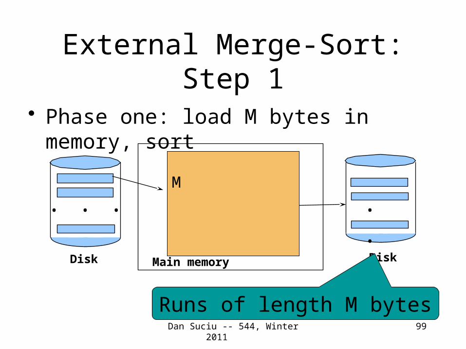
External Merge-Sort: Step 1
• Phase one: load M bytes in memory, sort
DiskDisk
. .
.. . .
M
Main memory
Runs of length M bytes
Dan Suciu -- 544, Winter 2011
100
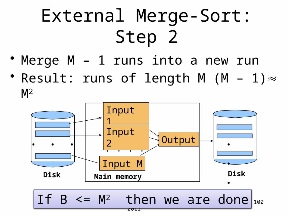
External Merge-Sort: Step 2
• Merge M – 1 runs into a new run• Result: runs of length M (M – 1) M2
DiskDisk
. .
.. . .
Input M
Input 1
Input 2. . . .
Output
Main memory
Dan Suciu -- 544, Winter 2011 If B <= M2 then we are done

101
Cost of External Merge Sort
• Read+write+read = 3B(R)
• Assumption: B(R) <= M2
Dan Suciu -- 544, Winter 2011
102
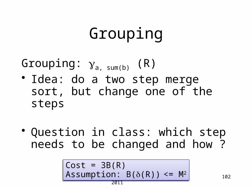
Grouping
Grouping: ga, sum(b) (R)• Idea: do a two step merge sort, but
change one of the steps
• Question in class: which step needs to be changed and how ?
Dan Suciu -- 544, Winter 2011
Cost = 3B(R)Assumption: B(d(R)) <= M2

103
Merge-Join
Join R ⨝ S• Step 1a: initial runs for R• Step 1b: initial runs for S• Step 2: merge and join
Dan Suciu -- 544, Winter 2011

104
Merge-Join
Main memory
DiskDisk
. .
.. . .
Input M
Input 1
Input 2. . . .
Output
M1 = B(R)/M runs for RM2 = B(S)/M runs for SMerge-join M1 + M2 runs; need M1 + M2 <= M

105
Two-Pass Algorithms Based on Sorting
Join R ⨝ S• If the number of tuples in R matching
those in S is small (or vice versa) we can compute the join during the merge phase
• Total cost: 3B(R)+3B(S) • Assumption: B(R) + B(S) <= M2
Dan Suciu -- 544, Winter 2011
106
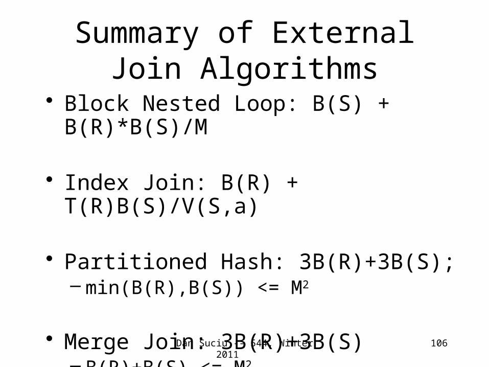
Summary of External Join Algorithms
• Block Nested Loop: B(S) + B(R)*B(S)/M
• Index Join: B(R) + T(R)B(S)/V(S,a)
• Partitioned Hash: 3B(R)+3B(S);– min(B(R),B(S)) <= M2
• Merge Join: 3B(R)+3B(S)– B(R)+B(S) <= M2
Dan Suciu -- 544, Winter 2011