1

COMP 578Artificial Neural Networks

for Data Mining

Keith C.C. Chan

Department of Computing

The Hong Kong Polytechnic University

2

Human vs. Computer• Computers

– Not good at performing such tasks as visual or audio processing/recognition.

– Execute instructions one after another extremely rapidly.

– Good at serial activities (e.g. counting, adding).

• Human brain– Units respond at 10/s (vs. PV 2.5GHz).

– Work on many different things at once.

– Vision or speech recognition by interaction of many different pieces of information.

3

The brain• Human brain is complicated and poorly understood.• Contains approximately 1010 basic units called

neurons.• Each neuron connected to about 10,000 others.

Axon

Dendrites

Synapse

Soma (or Cell Body)

4

The Neuron

• Neuron accepts many inputs (through dendrites).

• Inputs are all added up in some fashion.

• If enough active inputs are received at once, neuron will be activated and “fire” (through axon).

Dendrites

AxonSoma

Synapse

5

The Synapse• Axon produce voltage pulse

called action potential (AP).• Need arrival of more than

one AP to trigger synapse.• Synapse releases

neurotransmitters when AP is raised sufficiently.

• Neurotransmitters diffuse across the gap chemically activating dendrites on the other side.

• Some synapses pass a large signal across, whilst others allow very little through.

6

Modeling the Single Neuron• n inputs.• Efficiency of synapses

modeled by having a multiplicative factor on each of the inputs to the neuron.

• Multiplicative factor = associated weights on input lines.

• Neuron’s tasks:– Calculates weighted

sum of its inputs.– Compares sum to

some internal threshold.

– Turn on if threshold exceeded.

Σ

x1

x2

xn

w1

w2

wn

y

7

A Mathematical Model of Neurons• Neuron computes

weighted sum:

• Fire if SUM exceeds a threshold θ.– y=1 if SUM > θ– y=0 if SUM θ.

n

iii xwSUM

1

8

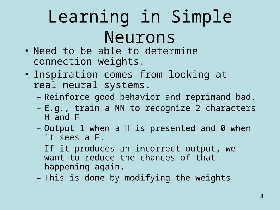
Learning in Simple Neurons• Need to be able to determine connection

weights.• Inspiration comes from looking at real neural

systems.– Reinforce good behavior and reprimand bad.– E.g., train a NN to recognize 2 characters H and F– Output 1 when a H is presented and 0 when it

sees a F.– If it produces an incorrect output, we want to

reduce the chances of that happening again.– This is done by modifying the weights.

9

Learning in Simple Neurons (2)• Neuron given random initial weights.

– At starting state, neuron knows nothing.

• Present an H.– Neuron computes the weighted sum of inputs.– Compare weighted sum with threshold.– If exceeds threshold, output a 1 otherwise a 0.

• If output is 1, neuron is correct.– Do nothing.

• Otherwise if neuron produces a 0.– Increase the weights so that next time it will exceed

the threshold and produces a 1.

10

A Simple Learning Rule

• How much weight to increase?• Can follow simple rule:

– Add the input values to the weights when we want the output to be on.

– Subtract the input values from the weights when we want the output to be off.

• This learning rule is called the Hebb rule:– It is a variant on one proposed by Donald Hebb and is

called Hebbian learning.– It is the earliest and simplest learning rule for a

neuron.

11

The Hebb Net

• Step 0. Initialize all weights:– wi =0 (i = 1 to n).

• Step 1. For each input training record (s) it’s target output (t), do steps 2-4.– Step 2. Set activations for all input units:– Step 3. Set activation for the output unit:– Step 4. Adjust the weights and the bias:

• wi (new) = wi (old) + xi y (i = 1 to n) (note: wi = xi y)• θ(new) = θ(old) + y .

• The bias (the θ) adjusted like a weight from a unit whose output signal is always 1.

12

A Hebb Net Example

13

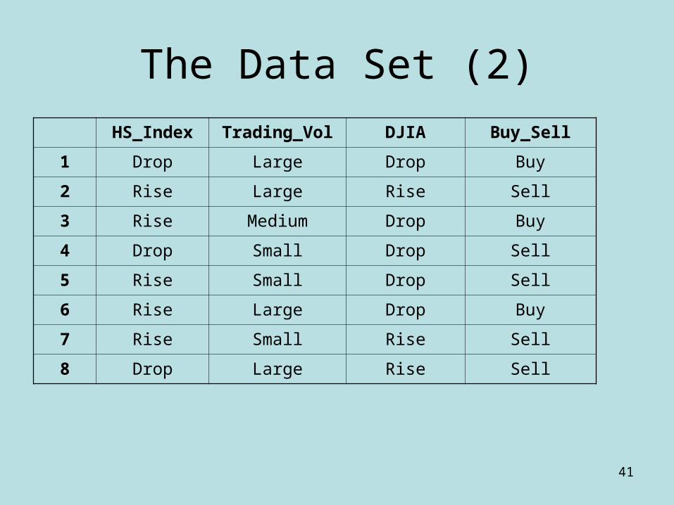
The Data Set

• Attributes– HS_Index: {Drop, Rise}– Trading_Vol: {Small, Medium, Large}– DJIA: {Drop, Rise}

• Class Label– Buy_Sell: {Buy, Sell}

14

The Data Set

HS_Index Trading_Vol DJIA Buy_Sell

1 Drop Large Drop Buy

2 Rise Large Rise Sell

3 Rise Medium Drop Buy

4 Drop Small Drop Sell

5 Rise Small Drop Sell

6 Rise Large Drop Buy

7 Rise Small Rise Sell

8 Drop Large Rise Sell

15

Transformation

• Input Features– HS_Index_Drop: {-1, 1}– HS_Index_Rise: {-1, 1}– Trading_Vol_Small: {-1, 1}– Trading_Vol_Medium: {-1, 1}– Trading_Vol_Large: {-1, 1}– DJIA_Drop: {-1, 1}– DJIA_Rise: {-1, 1}– Bias: {1}

• Output Feature– Buy_Sell: {-1, 1}

HIS=Drop

HIS=Rise

Bias

DJIA=Drop

DJIA=Rise

B/S

16

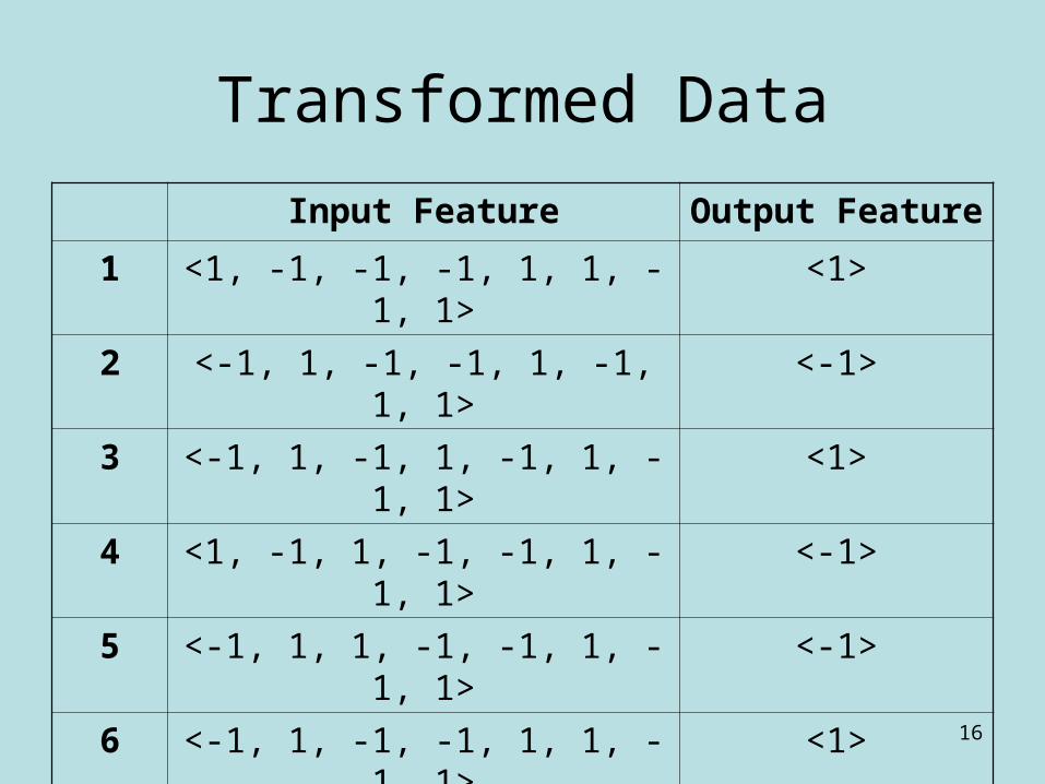
Transformed Data

Input Feature Output Feature

1 <1, -1, -1, -1, 1, 1, -1, 1> <1>

2 <-1, 1, -1, -1, 1, -1, 1, 1> <-1>

3 <-1, 1, -1, 1, -1, 1, -1, 1> <1>

4 <1, -1, 1, -1, -1, 1, -1, 1> <-1>

5 <-1, 1, 1, -1, -1, 1, -1, 1> <-1>

6 <-1, 1, -1, -1, 1, 1, -1, 1> <1>

7 <-1, 1, 1, -1, -1, -1, 1, 1> <-1>

8 <1, -1, -1, -1, 1, -1, 1, 1> <-1>

17

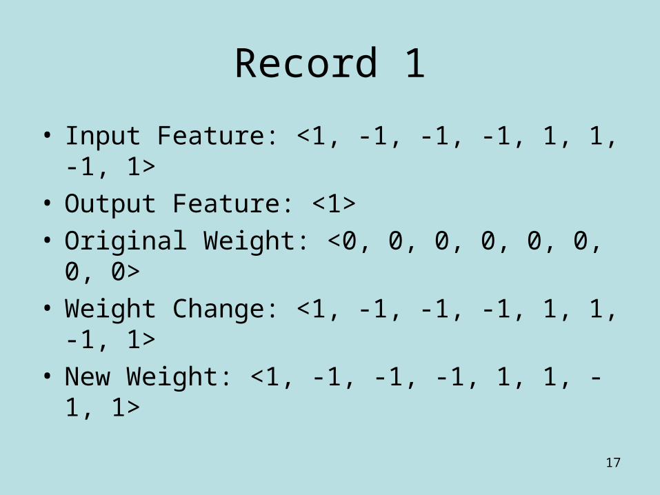
Record 1

• Input Feature: <1, -1, -1, -1, 1, 1, -1, 1>• Output Feature: <1>• Original Weight: <0, 0, 0, 0, 0, 0, 0, 0>• Weight Change: <1, -1, -1, -1, 1, 1, -1, 1>• New Weight: <1, -1, -1, -1, 1, 1, -1, 1>

18

Record 2

• Input Feature: <-1, 1, -1, -1, 1, -1, 1, 1>• Output Feature: <-1>• Original Weight: <1, -1, -1, -1, 1, 1, -1, 1>• Weight Change: <1, -1, 1, 1, -1, 1, -1, -1>• New Weight: <2, -2, 0, 0, 0, 2, -2, 0>

19

Record 3

• Input Feature: <-1, 1, -1, 1, -1, 1, -1, 1>• Output Feature: <1>• Original Weight: <2, -2, 0, 0, 0, 2, -2, 0>• Weight Change: <-1, 1, -1, 1, -1, 1, -1, 1>• New Weight: <1, -1, -1, 1, -1, 3, -3, 1>

20

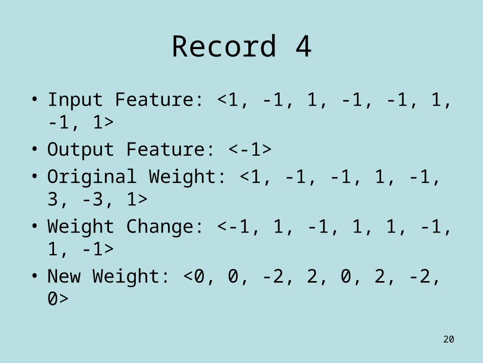
Record 4

• Input Feature: <1, -1, 1, -1, -1, 1, -1, 1>• Output Feature: <-1>• Original Weight: <1, -1, -1, 1, -1, 3, -3, 1>• Weight Change: <-1, 1, -1, 1, 1, -1, 1, -1>• New Weight: <0, 0, -2, 2, 0, 2, -2, 0>

21

Record 5

• Input Feature: <-1, 1, 1, -1, -1, 1, -1, 1>• Output Feature: <-1>• Original Weight: <0, 0, -2, 2, 0, 2, -2, 0>• Weight Change: <1, -1, -1, 1, 1, -1, 1, -1>• New Weight: <1, -1, -3, 3, 1, 1, -1, -1>

22

Record 6

• Input Feature: <-1, 1, -1, -1, 1, 1, -1, 1>• Output Feature: <1>• Original Weight: <1, -1, -3, 3, 1, 1, -1, -1>• Weight Change: <-1, 1, -1, -1, 1, 1, -1, 1>• New Weight: <0, 0, -4, 2, 2, 2, -2, 0>

23

Record 7

• Input Feature: <-1, 1, 1, -1, -1, -1, 1, 1>• Output Feature: <-1>• Original Weight: <0, 0, -4, 2, 2, 2, -2, 0>• Weight Change: <1, -1, -1, 1, 1, 1, -1, -1>• New Weight: <1, -1, -5, 3, 3, 3, -3, -1>

24

Record 8

• Input Feature: <1, -1, -1, -1, 1, -1, 1, 1>• Output Feature: <-1>• Original Weight: <1, -1, -5, 3, 3, 3, -3, -1>• Weight Change: <-1, 1, 1, 1, -1, 1, -1, -1>• New Weight: <0, 0, -4, 4, 2, 4, -4, -2>

25

A Hebb Net Example 2

(x1 X2 1)

(1 1 1) +1

(1 -1 1) -1

(-1 1 1) -1

(-1 -1 1) -1

Input Target

26

(x1 x2 1) (w` w2 θ) (w1 w2 θ)

(0 0 0)

(1 1 1) 1 (1 1 1) (1 1 1)

Input Target Weight Changes Weights

The separating line becomes x2 = - x1 - 1

x2

x1

27

(x1 x2 1) (w1 w2 b) (w1 w2 b)

(1 1 1)

(1 -1 1) -1 (-1 1 -1) (0 2 0)

Input Target Weight Changes Weights

The separating line becomesx2 = 0

x2

x1

28

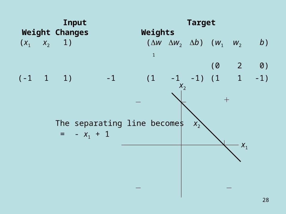
(x1 x2 1) (w1 w2 b) (w1 w2 b)

(0 2 0)

(-1 1 1) -1 (1 -1 -1) (1 1 -1)

Input Target Weight Changes Weights

The separating line becomes x2 = - x1 + 1

x2

x1

29

(x1 x2 1) (w1 w2 b) (w1 w2 b)

(1 1 -1)

(-1 -1 1) -1 (1 1 -1) (2 2 -2)

Input Target Weight Changes Weights

Even though the weights have changed, the separating line is still x2 = - x1 + 1

The graph of the decision regions (the positive response and the negative response) remains as shown.

x1

x2

30

A Hebb Net Example 3

(x1 x2 1)

(1 1 1) 1

(1 0 1) 0

(0 1 1) 0

(0 0 1) 0

Input Target

31

(x1 x2 1) (w1 w2 b) (w1 w2 b)

(0 0 0)

(1 1 1) 1 (1 1 1) (1 1 1)

Input Target Weight Changes Weights

The separating line becomesx2 = - x1 - 1

x2

00

0

x1

32

(x1 x2 1) (w1 w2 b) (w1 w2 b)

(1 0 1) 0 (0 0 0) (1 1 1)

(0 1 1) 0 (0 0 0) (1 1 1)

(0 0 1) 0 (0 0 0) (1 1 1)

Input Target Weight Changes Weights

Since the target value is 0, no learning occurs.

Using binary target values prevents the net from learning any pattern for which the target is “off”.

33

Characteristics of the Hebb Net

• Choice of training records determines which problems can be solved.

• Training records corresponding to the AND function can be solved if inputs and targets in bipolar form.

• Bipolar representation allows modification of a weight when input and target are both “on” and when they are both “off” at the same time.

34

The Perceptron Learning Rule• More powerful than the Hebb rule.• The Perceptron learning rule convergence

theorem states that:– If weights exist to allow neuron to respond correctly

to all training patterns, then the rule will find such weights.

– The neuron will find these weights in a finite number of training steps.

• Let SUM be the weighted sum, the output of the Perceptron, y = f(SUM), can be 1, 0, -1.

• The activation function is:

θ

θθ

θ

SUM

SUM-

SUM

SUMf

,1

,0

,1

)(

35

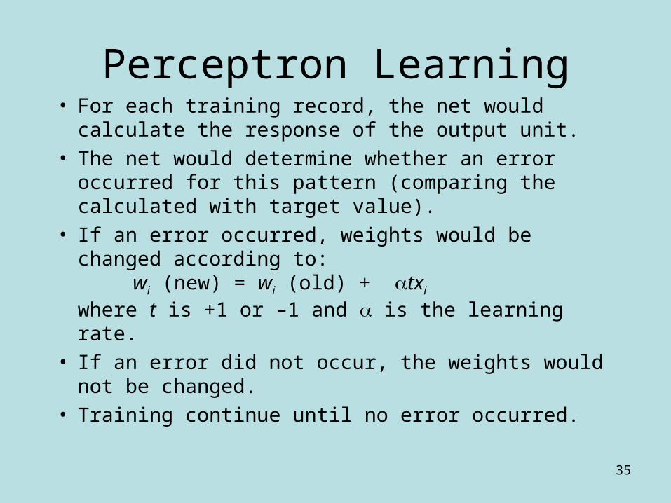
Perceptron Learning• For each training record, the net would calculate the

response of the output unit.• The net would determine whether an error occurred

for this pattern (comparing the calculated with target value).

• If an error occurred, weights would be changed according to:

wi (new) = wi (old) + txi

where t is +1 or –1 and is the learning rate.• If an error did not occur, the weights would not be

changed.• Training continue until no error occurred.

36

Perceptron for classification• Step 0. Initialize all weights and bias:

(For simplicity, set weights and bias to zero.)Set learning rate (0 < < 1). (For simplicity, can be set to 1.)

• Step 1. While stopping condition is false, do steps 2-6.• Step 2. For each training pair, do Steps 3-5:• Step 3. Set activation for input unit, xi.• Step 4. Compute response of output unit:

SUM = θ + i xi wi.• Step 5. Update weights and bias if error occurred for this

vector.If y’ y, wi (new) = wi (old) + txi θ(new) = θ (old) + t else wi (new) = wi (old) θ (new) = θ (old)

• Step 6. If no weights changed in 2, stop else continue.

37

Perceptron for classification (2)

• Only weights connecting active input units (xi0) are updated.

• Weights are updated only for patterns that do not produce the correct value of y.

• Less learning as more training patterns produce the correct response.

• The threshold on the activation function for the response unit is a fixed, non-negative value .

• The form of the activation function for the output unit constitutes an undecided band of fixed width determined by separating the region of positive response from that of negative response.

38

Perceptron for classification (3)

• Instead of one separating line, we have a line separating the region of positive response from the region of zero response (line bounding inequality):– w1 x1 + w2 x2 + b >

• and a line separating the region of zero response from the region of negative response (line bounding the inequality):

w1 x1 + w2 x2 + b <

w1 x1 + w2 x2 + b >

w1 x1 + w2 x2 + b <

39

Perceptron

40

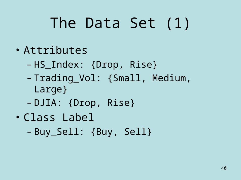
The Data Set (1)

• Attributes– HS_Index: {Drop, Rise}– Trading_Vol: {Small, Medium, Large}– DJIA: {Drop, Rise}

• Class Label– Buy_Sell: {Buy, Sell}

41

The Data Set (2)

HS_Index Trading_Vol DJIA Buy_Sell

1 Drop Large Drop Buy

2 Rise Large Rise Sell

3 Rise Medium Drop Buy

4 Drop Small Drop Sell

5 Rise Small Drop Sell

6 Rise Large Drop Buy

7 Rise Small Rise Sell

8 Drop Large Rise Sell

42

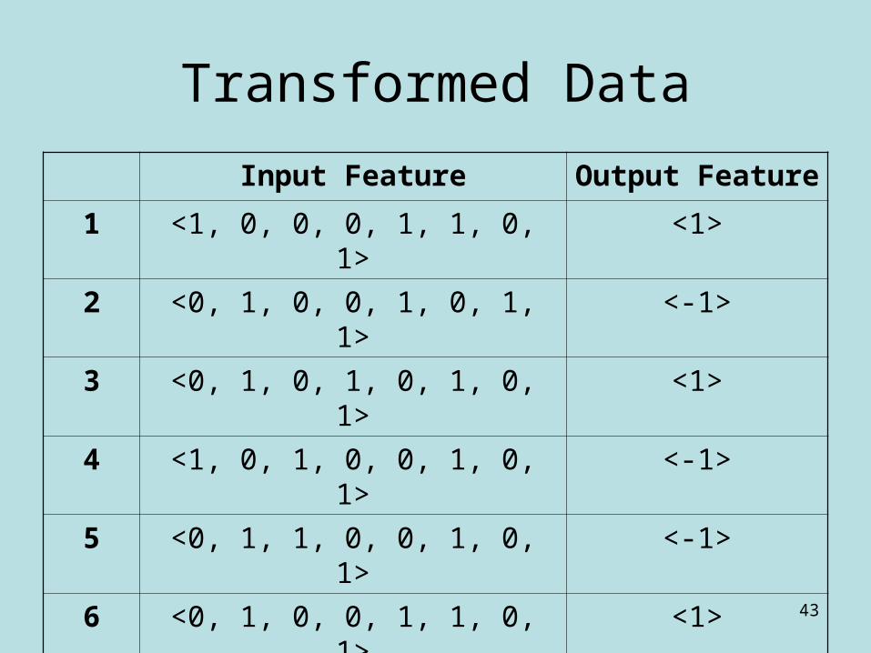
Transformation

• Input Features– HS_Index_Drop: {0, 1}– HS_Index_Rise: {0, 1}– Trading_Vol_Small: {0, 1}– Trading_Vol_Medium: {0, 1}– Trading_Vol_Large: {0, 1}– DJIA_Drop: {0, 1}– DJIA_Rise: {0, 1}– Bias: {0}

• Output Feature– Buy 1– Sell -1

43

Transformed Data

Input Feature Output Feature

1 <1, 0, 0, 0, 1, 1, 0, 1> <1>

2 <0, 1, 0, 0, 1, 0, 1, 1> <-1>

3 <0, 1, 0, 1, 0, 1, 0, 1> <1>

4 <1, 0, 1, 0, 0, 1, 0, 1> <-1>

5 <0, 1, 1, 0, 0, 1, 0, 1> <-1>

6 <0, 1, 0, 0, 1, 1, 0, 1> <1>

7 <0, 1, 1, 0, 0, 0, 1, 1> <-1>

8 <1, 0, 0, 0, 1, 0, 1, 1> <-1>

44

Record 1

• Input Feature: <1, 0, 0, 0, 1, 1, 0, 1>• Output Feature: <1>• Original Weight: <0, 0, 0, 0, 0, 0, 0, 0>• Output: f(0) = 0• Weight Change: <1, 0, 0, 0, 1, 1, 0, 1>• New Weight: <1, 0, 0, 0, 1, 1, 0, 1>

45

Record 2

• Input Feature: <0, 1, 0, 0, 1, 0, 1, 1>• Output Feature: <-1>• Original Weight: <1, 0, 0, 0, 1, 1, 0, 1>• Output: f(2) = 1• Weight Change: <0, -1, 0, 0, -1, 0, -1, -1>• New Weight: <1, -1, 0, 0, 0, 1, -1, 0>

46

Record 3

• Input Feature: <0, 1, 0, 1, 0, 1, 0, 1>• Output Feature: <1>• Original Weight: <1, -1, 0, 0, 0, 1, -1, 0>• Output: f(1) = 0• Weight Change: <0, 1, 0, 1, 0, 1, 0, 1>• New Weight: <1, 0, 0, 1, 0, 2, -1, 1>

47

Record 4

• Input Feature: <1, 0, 1, 0, 0, 1, 0, 1>• Output Feature: <-1>• Original Weight: <1, 0, 0, 1, 0, 2, -1, 1>• Output: f(4) = 1• Weight Change: <-1, 0, -1, 0, 0, -1, 0, -1>• New Weight: <0, 0, -1, 1, 0, 1, -1, 0>

48

Record 5

• Input Feature: <0, 1, 1, 0, 0, 1, 0, 1>• Output Feature: <-1>• Original Weight: <0, 0, -1, 1, 0, 1, -1, 0>• Output: f(0) = 0• Weight Change: <0, -1, -1, 0, 0, -1, 0, -1>• New Weight: <0, -1, -2, 1, 0, 0, -1, -1>

49

Record 6

• Input Feature: <0, 1, 0, 0, 1, 1, 0, 1>• Output Feature: <1>• Original Weight: <0, -1, -2, 1, 0, 0, -1, -1>• Output: f(-2) = -1• Weight Change: <0, 1, 0, 0, 1, 1, 0, 1>• New Weight: <0, 0, -2, 1, 1, 1, -1, 0>

50

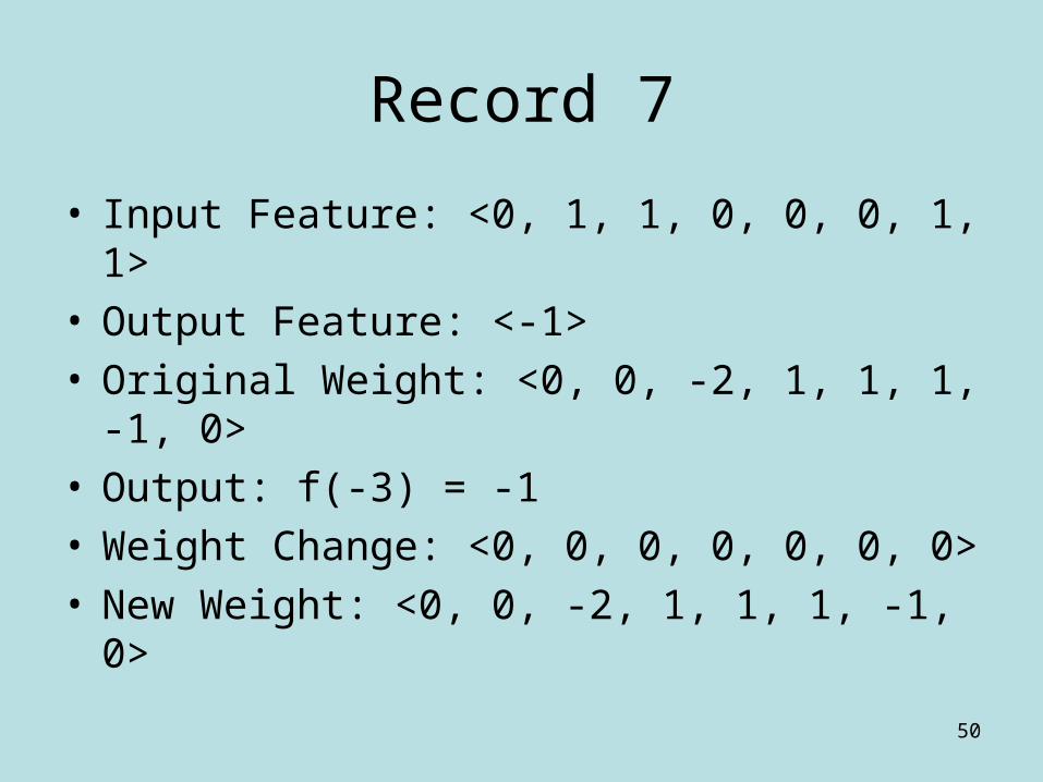
Record 7

• Input Feature: <0, 1, 1, 0, 0, 0, 1, 1>• Output Feature: <-1>• Original Weight: <0, 0, -2, 1, 1, 1, -1, 0>• Output: f(-3) = -1• Weight Change: <0, 0, 0, 0, 0, 0, 0>• New Weight: <0, 0, -2, 1, 1, 1, -1, 0>

51

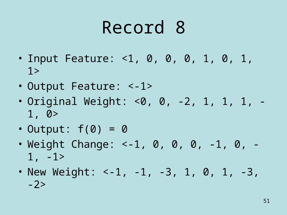
Record 8

• Input Feature: <1, 0, 0, 0, 1, 0, 1, 1>• Output Feature: <-1>• Original Weight: <0, 0, -2, 1, 1, 1, -1, 0>• Output: f(0) = 0• Weight Change: <-1, 0, 0, 0, -1, 0, -1, -1>• New Weight: <-1, -1, -3, 1, 0, 1, -3, -2>

52

A Perceptron Example

(x1 x2 1)

(1 1 1) 1

(1 0 1) -1

(0 1 1) -1

(0 0 1) -1

53

(x1 x2 1) (w1 w2 b)

(0 0 0)

(1 1 1) 0 0 1 (1 1 1) (1 1 1)

Input Net Out Target Weight Changes Weights

The separating lines becomex1 + x2 + 1 = .2

andx1 + x2 + 1 = -.2

x2

x1

54

The separating lines becomex2 = .2

and x2 = -.2

(x1 x2 1) (w1 w2 b)

(1 1 1)

(1 0 1) 2 1 -1 (-1 0 -1) (0 1 0)

Input Net Out Target Weight Changes Weights

x2

x1

55

(x1 x2 1) (w1 w2 b)

(0 1 0)

(0

(0

1

0

1)

1)

1

-1

1

-1

-1

-1

(0

(0

-1

0

-1)

0)

(0

(0

0

0

-1)

-1)

Input Net Out Target Weight Changes Weights

56

(x1 x2 1) (w1 w2 b)

(0 0 -1)

(1 1 1) -1 -1 1 (1 1 1) (1 1 0)

Input Net Out Target Weight Changes Weights

The separating line become x1 + x2 = .2

and x1 + x2 = -.2

x2

x1

57

(x1 x2 1) (w1 w2 b)

(1 1 0)

(1 0 1) 1 1 -1 (-1 0 -1) (0 1 -1)

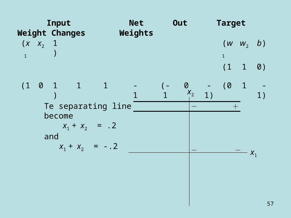
Input Net Out Target Weight Changes Weights

Te separating line become x1 + x2 = .2

and x1 + x2 = -.2

x2

x1

58

(x1 x2 1) (w1 w2 b)

(0 1 -1)

(0

(0

1

0

1)

1)

0

-2

0

-1

-1

-1

(0

(0

-1

0

-1)

0)

(0

(0

0

0

-2)

-2)

Input Net Out Target Weight Changes Weights

The results for the third epoch are:

(x1 x2 1) (w1 w2 b)

(0 0 -2)

(1 1 1) -2 -1 1 (1 1 1) (1 1 -1)

(1 0 1) 0 0 -1 (-1 0 -1) (0 1 -1)

(0 1 1) -1 -1 -1 (0 0 0) (0 1 -2)

(0 0 1) -2 -1 -1 (0 0 0) (0 1 -2)

Input Net Out Target Weight Changes Weights

59

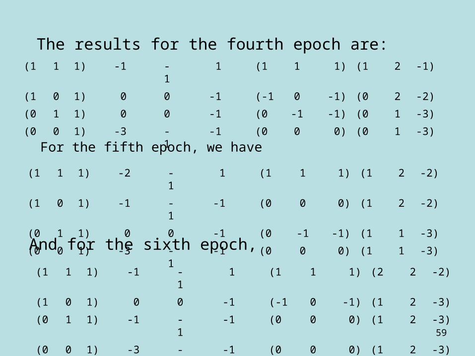
The results for the fourth epoch are:

(1 1 1) -1 -1 1 (1 1 1) (1 2 -1)

(1 0 1) 0 0 -1 (-1 0 -1) (0 2 -2)

(0 1 1) 0 0 -1 (0 -1 -1) (0 1 -3)

(0 0 1) -3 -1 -1 (0 0 0) (0 1 -3)

For the fifth epoch, we have

(1 1 1) -2 -1 1 (1 1 1) (1 2 -2)

(1 0 1) -1 -1 -1 (0 0 0) (1 2 -2)

(0 1 1) 0 0 -1 (0 -1 -1) (1 1 -3)

(0 0 1) -3 -1 -1 (0 0 0) (1 1 -3)

And for the sixth epoch,

(1 1 1) -1 -1 1 (1 1 1) (2 2 -2)

(1 0 1) 0 0 -1 (-1 0 -1) (1 2 -3)

(0 1 1) -1 -1 -1 (0 0 0) (1 2 -3)

(0 0 1) -3 -1 -1 (0 0 0) (1 2 -3)

60

(1 1 1) 0 0 1 (1 1 1) (2 3 -2)

(1 0 1) 0 0 -1 (-1 0 -1) (1 3 -3)

(0 1 1) 0 0 -1 (0 -1 -1) (1 2 -4)

(0 0 1) -4 -1 -1 (0 0 0) (1 2 -4)

The results for the seventh epoch are:

The eight epoch yields(1 1 1) -1 -1 1 (1 1 1) (2 3 -3)

(1 0 1) -1 -1 -1 (0 0 0) (2 3 -3)

(0 1 1) 0 0 -1 (0 -1 -1) (2 2 -4)

(0 0 1) -4 -1 -1 (0 0 0) (2 2 -4)

(1 1 1) 0 0 1 (1 1 1) (3 3 -3)

(1 0 1) 0 0 -1 (-1 0 -1) (2 3 -4)

(0 1 1) -1 -1 -1 (0 0 0) (2 3 -4)

(0 0 1) -4 -1 -1 (0 0 0) (2 3 -4)

And the ninth

61

Finally, the results for the tenth epoch are

(1 1 1) 1 1 1 (0 0 0) (2 3 -4)

(1 0 1) -2 -1 -1 (0 0 0) (2 3 -4)

(0 1 1) -1 -1 -1 (0 0 0) (2 3 -4)

(0 0 1) -4 -1 -1 (0 0 0) (2 3 -4)

• The positive response is given by:– 2x1 + 3x2 – 4 > .2

• with boundary line– x2 = -2 / 3x1 + 7 / 5

• The negative response is given by:– 2x1 + 3x2 – 4 < -.2

• with boundary line– x2 = -2 / 3x1 + 19 / 15

x2

x1

62

The 2nd Perceptron Algorithm

(x1 x2 1) (w1 w2 b)

(0 0 0)

(1 1 1) 0 0 1 (1 1 1) (1 1 1)

(1 -1 1) 1 1 -1 (-1 1 -1) (0 2 0)

(-1 1 1) 2 1 -1 (1 -1 -1) (1 1 -1)

(-1 -1 1) -3 -1 -1 (0 0 0) (1 1 -1)

Input Net Out Target Weight Changes Weights

63

In the second epoch of training, we have:

(1 1 1) 1 1 1 (0 0 0) (1 1 -1)

(1 -1 1) -1 -1

-1 (0 0 0) (1 1 -1)

(-1 1 1) -1 -1

-1 (0 0 0) (1 1 -1)

(-1 -1 1) -3 -1

-1 (0 0 0) (1 1 -1)Since all the w’s are 0 in epoch 2, the system was fully trained after the first epoch.

64

Limitations of Perceptrons

• Perceptron finds a straight line that separates classes.• It cannot learn for exclusive-or (XOR) problems.• Such patterns are not linearly separable.• Not much work after Minsky and Papert published their

book in 1969.• Rumelhart and McClelland produced an improvement in

1986.– Proposed some modern adaptations to Perceptron, called

multilayer Perceptron.

65

The Multilayer Perceptron• Overcome linearly

inseparability:– Use more perceptrons.– Each set up to identify

small, linearly separable sections of the inputs.

– Combine their outputs into another perceptron.

• Each neuron still takes weighted sum of inputs, thresholds it, outputs 1 or 0.

• But how can we learn?

66

The Multilayer Perceptron (2)

• Perceptrons in the 2nd layer do not know which of the real inputs were on or not.

• Only 2-state, on or off, gives no indication of how much to adjust the weights.– Some weighted input definitely turn on a neuron.– Some weighted inputs only just turn a neuron on and

should not be altered to the same extent. – What changes to produce a better solution next time?– Which of the input weights should be increased and

which should not?– But we have no way of finding out (the credit

assignment problem).

67

The Solution

• Need a non-binary thresholding function.

• Use a slightly different non-linearity so that it more or less turns on or off.

• A possible new thresholding function is the sigmoid function.

• Sigmoid thresholding function does not mask inputs from the outputs.

kxexf

1

1)(

68

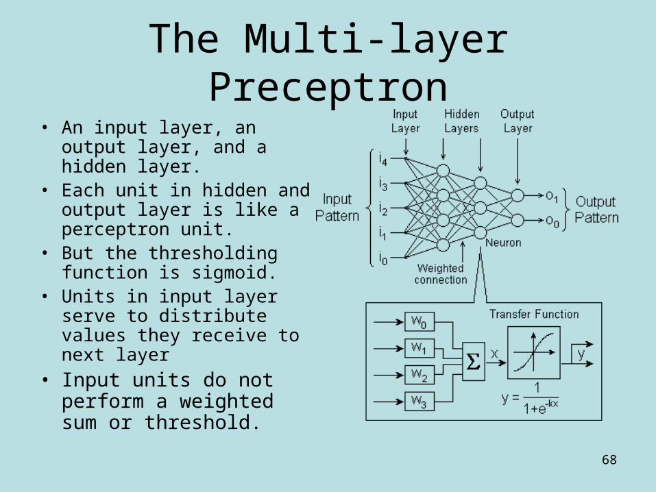
The Multi-layer Preceptron

• An input layer, an output layer, and a hidden layer.

• Each unit in hidden and output layer is like a perceptron unit.

• But the thresholding function is sigmoid.

• Units in input layer serve to distribute values they receive to next layer

• Input units do not perform a weighted sum or threshold.

69

The Backpropagation Rule

• Single-layer perceptron model changed.– Thresholding function from a step to a sigmoid

function.– A hidden layer added.– Learning rule needs to be altered.

• New learning rule for multilayer perceptron is called the “generalized delta rule”, or the “backpropagation rule”.– Show NN a pattern and calculate its response.– Compare with desired response.– Alter weights so that NN can produce a more accurate output

next time.– The learning rule provides the method for adjusting the weights

so as to decrease the error next time.

70

Backpropagation Details• Define an error function to represent difference between NN's

current output and the correct output.• The backpropagation rule aims to reduce the error by:

– Calculating the value of the error for a particular input.– Then back-propagates the error from one layer to the previous

one.– Each unit in the net has its weights adjusted so that it reduces

the value of the error function– For units on the output.

• Their output and desired output is known and adjusting the weights is relatively simple.

– For units in the middle:• Those that are connected to outputs with a large error should have their

weights adjusted a lot.• Those that feed almost correct outputs should not be altered much.

71

The Detailed Algorithm

• Step0. Initialize weights (Set to small random values). • Step 1. While stopping condition is false, do Steps 2-9.

– Step 2. For each training pair, do Steps 3-8.Feedbackward.

• Step 3. Each input unit (xi , i = 1, …, n) receives input signal xi and broadcasts this signal to all units in the layer above (the hidden units).

• Step 4. Each hidden unit (Zj , j = 1, …, p) sums its weighted input signals,

– applies its activation function to compute its output signal,

zj = f(z_inj),– and sends this signal to all units in the layer above (output units).

• Step 5. Each output unit (Yk , k=1, …, m) sums its weighted input signals,

– And applies its activation function to compute its output signal, yk = f(z_inj),

n

iijijj vxvinz

10_

p

jjkjkk wzwiny

10_

72

The Detailed Algorithm (2)Feedbackward.

• Step 6. Each output unit (yk , k = 1, …, m) receives a target pattern corresponding to the input training pattern, computes its error information term,

– Calculates its weight correction term (used to update wjk later),

wjk=kzj,– Calculates its bias correction term (used to upate w0k later),

w0k=k,– And sends k to units in the layer below.

• Step 7. Each hidden unit (Zj, j=1, …, p) sums its delta inputs (from units in the layer above),

– Multiplies by the derivative of its activation function to calculate its error information term,

j= _inj f’(z_inj),– Calculates its weight correction term (used to update vij later),

vij=jxi,

– And calculates its bias correction term (used to update v0j later),v0j=j,

),_(')( kkkk inyfyt

m

kjkk win

1

_

73

The Detailed Algorithm (3)

Update weights and biases:

• Step 8. Each output unit (Yk , k = 1, …, m) updates its bias and weights (j=0, …, p):

wjk(new)= wjk (old)+wjk ,

– Each hidden unit (Zj,j=1, …, p) updates its bias and weights (I=0,…,n):

vjk(new)= vjk (old)+vjk ,

– Step 9. Test stopping condition.

74

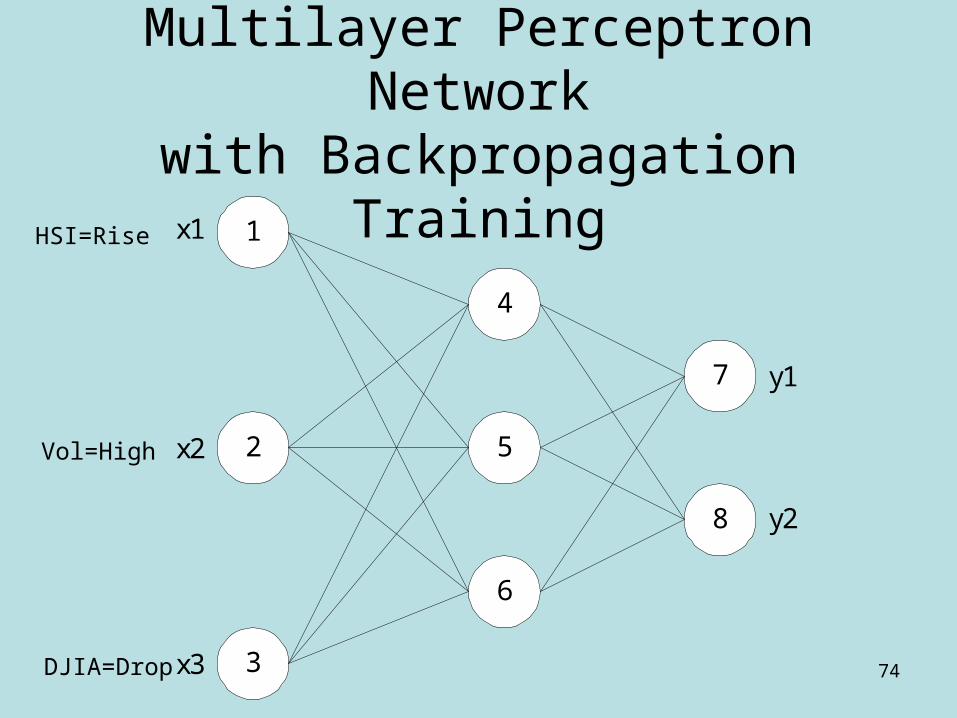
An example:Multilayer Perceptron Networkwith Backpropagation Training

1

4

52

3

6

x1

x2

x3

7

8

y1

y2

Vol=High

HSI=Rise

DJIA=Drop

75

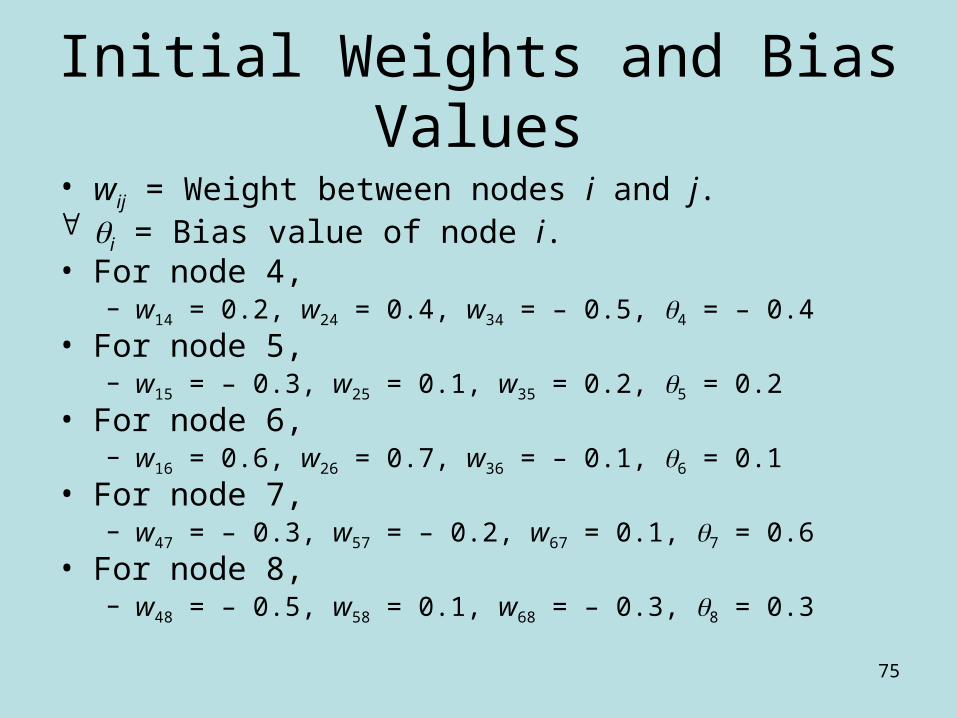
Initial Weights and Bias Values

• wij = Weight between nodes i and j. i = Bias value of node i.• For node 4,

– w14 = 0.2, w24 = 0.4, w34 = – 0.5, 4 = – 0.4• For node 5,

– w15 = – 0.3, w25 = 0.1, w35 = 0.2, 5 = 0.2• For node 6,

– w16 = 0.6, w26 = 0.7, w36 = – 0.1, 6 = 0.1• For node 7,

– w47 = – 0.3, w57 = – 0.2, w67 = 0.1, 7 = 0.6• For node 8,

– w48 = – 0.5, w58 = 0.1, w68 = – 0.3, 8 = 0.3

76

Training (1)• Learning Rate = 0.9• Input: <1, 0, 1>• Output: <1, 0>• For node 4,

– Input: 0.2 + 0 – 0.5 – 0.4 = – 0.7– Output: 1 / (1 + e 0.7) = 0.332

• For node 5,– Input: – 0.3 + 0 + 0.2 + 0.2 = 0.1– Output: 1 / (1 + e – 0.1) = 0.525

• For node 6,– Input: 0.6 + 0 – 0.1 + 0.1 = 0.6– Output: 1 / (1 + e – 0.6) = 0.646

• For node 7,– Input: 0.332 * (– 0.3) + 0.525 * (– 0.2) + 0.646 * 0.1 + 0.6 = 0.460– Output: 1 / (1 + e 0.460) = 0.613

• For node 8,– Input: 0.322 * (– 0.5) + 0.525 * 0.1 + 0.646 * (– 0.3) + 0.3 = – 0.007– Output: 1 / (1 + e – 0.007) = 0.498

77

Training (2)

• For node 7,– Error: 0.613 (1 – 0.613) (1 – 0.613) = 0.092

• For node 8,– Error: 0.498 (1 – 0.498) (0 – 0.498) = – 0.125

• For node 4,– Error: 0.332 (1 – 0.332) (0.092 * (– 0.3) + 0.125 * (– 0.5)) =

0.008• For node 5,

– Error: 0.525 (1 – 0.525) (0.092 * (– 0.2) + 0.125 * 0.1) = 0.009• For node 6,

– Error: 0.646 (1 – 0.646) (0.092 * 0.1 + 0.125 * (– 0.3)) = 0.008

78

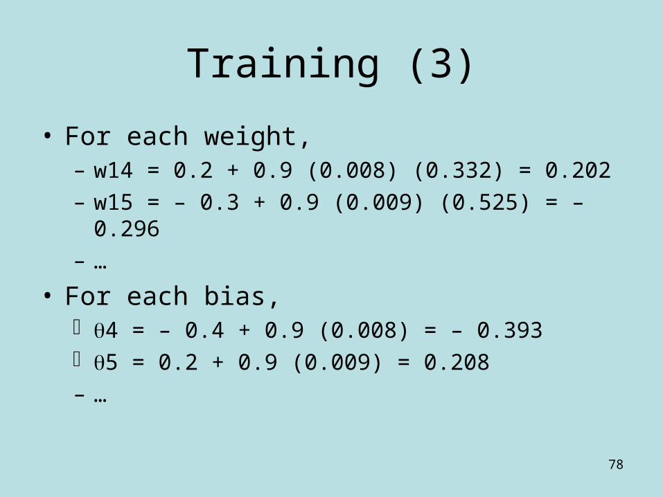
Training (3)

• For each weight,– w14 = 0.2 + 0.9 (0.008) (0.332) = 0.202– w15 = – 0.3 + 0.9 (0.009) (0.525) = – 0.296– …

• For each bias, 4 = – 0.4 + 0.9 (0.008) = – 0.393 5 = 0.2 + 0.9 (0.009) = 0.208– …

79

Using ANN for Data Mining • Constructing a network

– input data representation– selection of number of layers, number of

nodes in each layer

• Training the network using training data

• Pruning the network

• Interpret the results

80

Step 1: Constructing the Network

o2 Not-persist

o1 Persist

x3 Demographics

x2 GPA

w1

w5…n

x1 # of Terms

x4 Courses

x5 Fin Aid…

xj…n

Multi-layer perceptron (MLP): feed forward back propagation

81

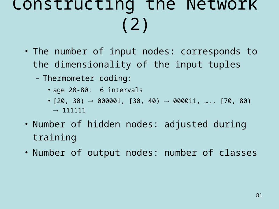
Constructing the Network (2)

• The number of input nodes: corresponds to the

dimensionality of the input tuples

– Thermometer coding: • age 20-80: 6 intervals

• [20, 30) 000001, [30, 40) 000011, …., [70, 80) 111111

• Number of hidden nodes: adjusted during

training

• Number of output nodes: number of classes

88

ANN vs. Others for Data Mining

• Advantages– prediction accuracy is generally high– robust, works when training examples contain errors– output may be discrete, real-valued, or a vector of

several discrete or real-valued attributes– fast evaluation of the learned target function.

• Criticism– long training time– difficult to understand the learned function (weights).– not easy to incorporate domain knowledge