1

Chapter 8Chapter 8

Sensitivity AnalysisSensitivity AnalysisChapter 8Chapter 8

Sensitivity AnalysisSensitivity Analysis

Bottom line:Bottom line: How does the optimal solution change as

some of the elements of the model change?

For obvious reasons we shall focus on For obvious reasons we shall focus on Linear Programming Models.Models.

2

Ingredients of LP ModelsIngredients of LP ModelsIngredients of LP ModelsIngredients of LP Models

Linear objective functionLinear objective function A system of linear constraintsA system of linear constraints

– RHS valuesRHS values

– Coefficient matrix (LHS)Coefficient matrix (LHS)

– Signs (=, <=, >=)Signs (=, <=, >=) How does the optimal solution change as

these elements change?

3

8.1 Introduction8.1 Introduction8.1 Introduction8.1 Introduction

What kind of changes are to be considered?What kind of changes are to be considered? How do we handle such changes?How do we handle such changes? To motivate the discussion it is instructive To motivate the discussion it is instructive

to classify the changes into two categories:to classify the changes into two categories:

– Structural changeschanges

– Parametric changeschanges

4

z * : = opt

x

cx : = cj

j = 1

n

∑ xj

Ax ~ b , A ∈ ℜm × n

, b ∈ ℜm

x ≥ 0

5

Structural ChangesStructural ChangesStructural ChangesStructural Changes

eg.eg. New decision variableNew decision variable New constraintNew constraint Loss of a decision variableLoss of a decision variable Relaxation of a constraintRelaxation of a constraint

6

Parametric ChangesParametric ChangesParametric ChangesParametric Changes

Changes in one or more of the coefficients Changes in one or more of the coefficients of the objective function (cof the objective function (c jj))

Changes in the RHS values (bChanges in the RHS values (b ii))

Changes in the coefficients of the LHS Changes in the coefficients of the LHS matrix {amatrix {aijij}.}.

7

our emphasis will be onour emphasis will be onour emphasis will be onour emphasis will be on

Basic principles and ideas rather than rather than investigation of many specific cases (as investigation of many specific cases (as done in many textbooks ....)done in many textbooks ....)

Thus, in the exam you may have to Thus, in the exam you may have to demonstrate that you know how to apply demonstrate that you know how to apply the principles to solve “new” problems.the principles to solve “new” problems.

8

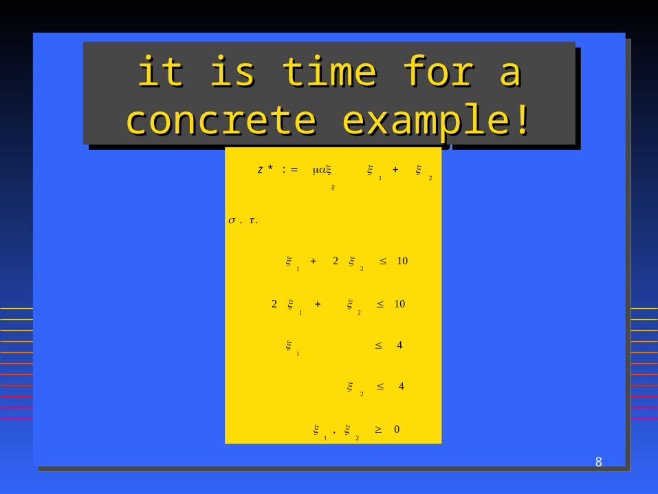
it is time for a concrete it is time for a concrete example!example!

it is time for a concrete it is time for a concrete example!example!z * : = max

x

x1

+ x2

s . t .

x1

+ 2 x2

≤ 10

2 x1

+ x2

≤ 10

x1

≤ 4

x2

≤ 4

x1, x

2≥ 0

9

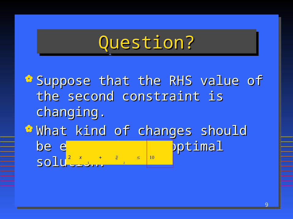
Question?Question?Question?Question?

Suppose that the RHS value of the second Suppose that the RHS value of the second constraint is changing.constraint is changing.

What kind of changes should be expect in What kind of changes should be expect in the optimal solution?the optimal solution?

2 x1

+ x2

≤ 10

10

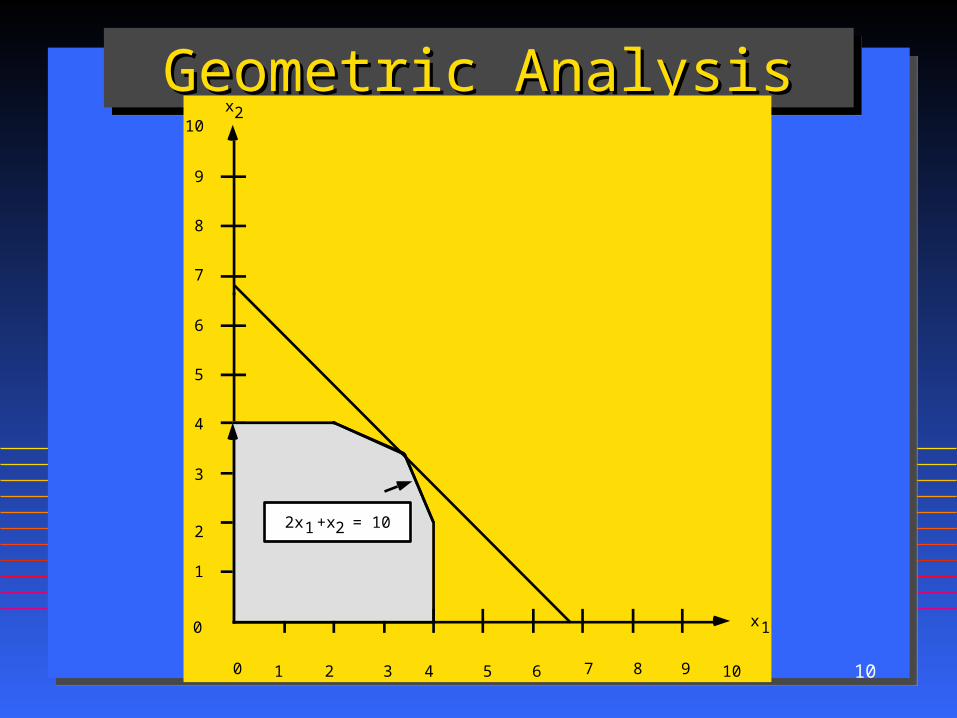
Geometric AnalysisGeometric AnalysisGeometric AnalysisGeometric Analysis

0 1 2 3 4 5 6 7 8 9 10

0

1

2

3

4

5

6

7

8

9

10x2

x1

2x1+x2 = 10

11

0 1 2 3 4 5 6 7 8 9 10

0

1

2

3

4

5

6

7

8

9

10x2

x1

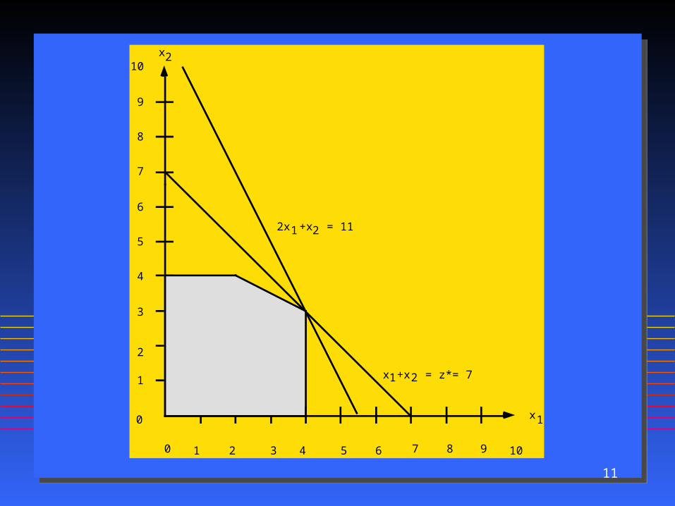
x1+x2 = z*= 7

2x1+x2 = 11

12

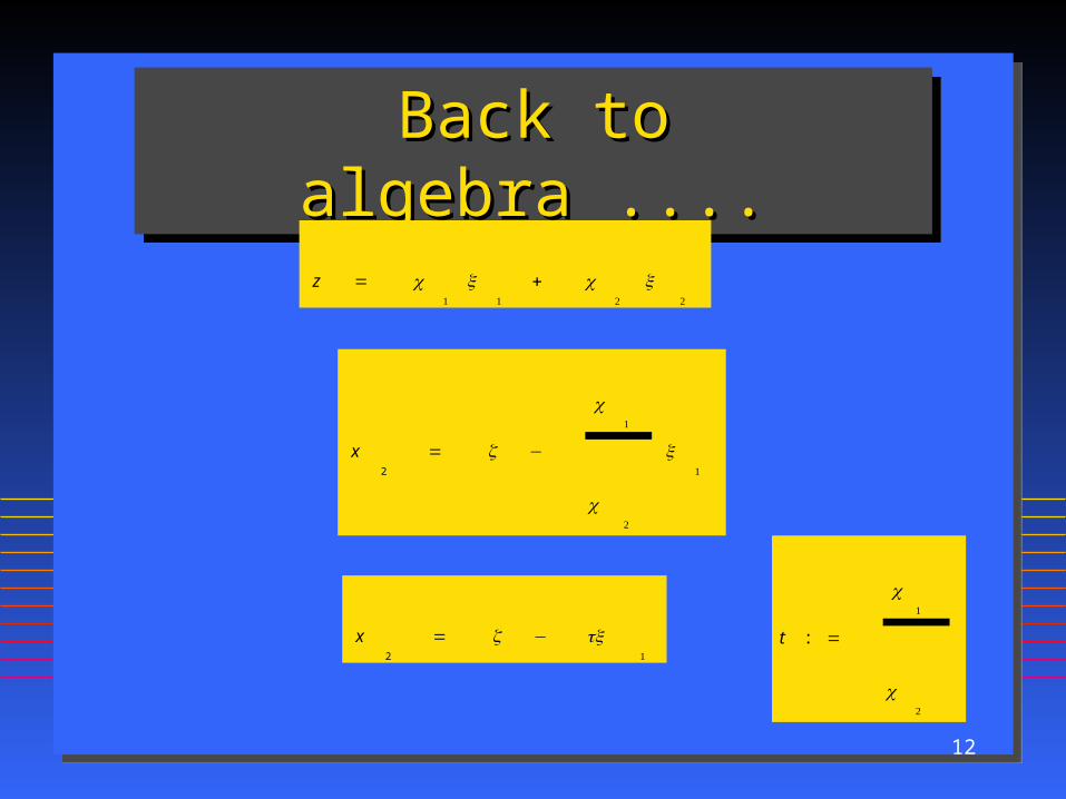
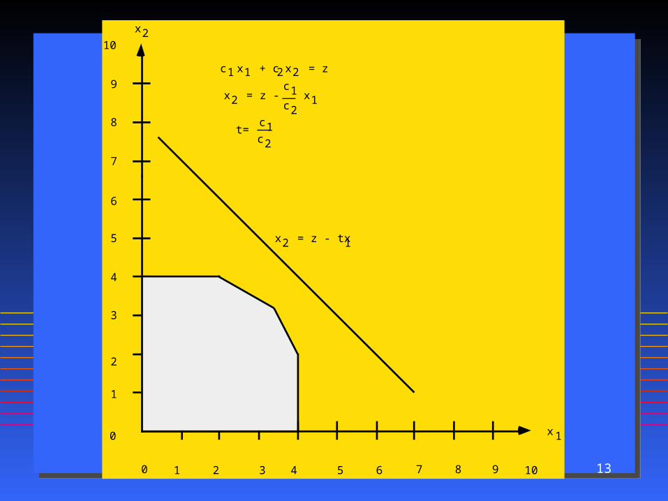
Back to algebra ....Back to algebra ....Back to algebra ....Back to algebra ....

z = c1

x1

+ c2

x2

x2

= z −

c1

c2

x1

x2

= z − tx1

t : =

c1

c2

130 1 2 3 4 5 6 7 8 9 10

0

1

2

3

4

5

6

7

8

9

10

x2

x 1

c1 x1 + c2x2 = z

t= __c2

c1

x2 = z - __c2

c1 x1

x2 = z - tx 1

140 1 2 3 4 5 6 7 8 9 10

0

1

2

3

4

5

6

7

8

9

10x 2

x 1

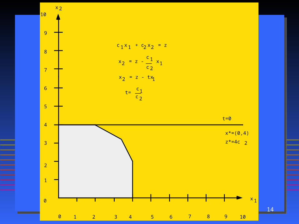
t=0

c 1x 1 + c 2 x2 = z

t= __c 2

c1

x2 = z - __c 2

c 1 x1

x2 = z - tx 1

x*=(0,4)

z*=4c 2

150 1 2 3 4 5 6 7 8 9 10

0

1

2

3

4

5

6

7

8

9

10x 2

x 1

t= __12

c 1 x 1 + c 2 x 2 = z

t= __c 2

c 1

x 2 = z - __c2

c1 x 1

x 2 = z - tx 1

z*=2c 1 +4c 2

160 1 2 3 4 5 6 7 8 9 10

0

1

2

3

4

5

6

7

8

9

10

x2

x1

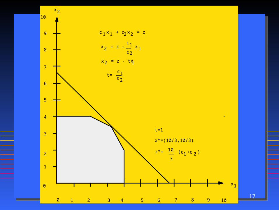
t=1

c 1x 1 + c 2x2 = z

t= __c2

c1

x2 = z - __c2

c1 x 1

x2 = z - tx 1

x*=(10/3,10/3)

z*= __10

3(c 1+c2 )

170 1 2 3 4 5 6 7 8 9 10

0

1

2

3

4

5

6

7

8

9

10

x2

x1

t=1

c 1x 1 + c 2x2 = z

t= __c2

c1

x2 = z - __c2

c1 x 1

x2 = z - tx 1

x*=(10/3,10/3)

z*= __10

3(c 1+c2 )

180 1 2 3 4 5 6 7 8 9 10

0

1

2

3

4

5

6

7

8

9

10x 2

x 1

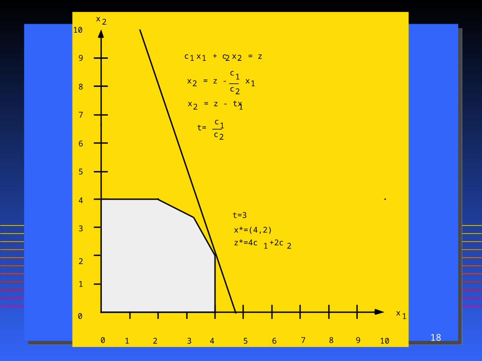
t=3

c1 x1 + c2 x2 = z

t= __c2

c1

x2 = z - __c2

c1 x1

x2 = z - tx 1

x*=(4,2)

z*=4c 1+2c2

190 1 2 3 4 5 6 7 8 9 10

0

1

2

3

4

5

6

7

8

9

10x2

x1

2x 1+x2 <=10

t= very large ....

c1x1 + c2x2 = z

t= __c2

c1

x2 = z - __c2

c1 x1

x2 = z - tx 1

x*=(4,0)

z*=4c 1

20

How do we conduct such an analysis in higher dimensions?

21

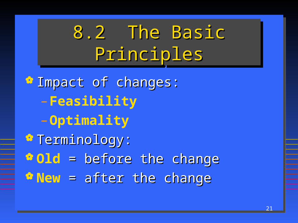
8.2 The Basic Principles8.2 The Basic Principles8.2 The Basic Principles8.2 The Basic Principles

Impact of changes:Impact of changes:

– Feasibility

– Optimality Terminology:Terminology: Old = before the change = before the change New = after the change = after the change

22

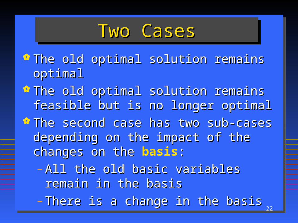
Two CasesTwo CasesTwo CasesTwo Cases The old optimal solution remains optimal The old optimal solution remains optimal The old optimal solution remains feasible but The old optimal solution remains feasible but

is no longer optimalis no longer optimal The second case has two sub-cases The second case has two sub-cases

depending on the impact of the changes on depending on the impact of the changes on the the basis::

– All the old basic variables remain in the All the old basic variables remain in the basisbasis

– There is a change in the basisThere is a change in the basis

23

The latter means that a number of pivot The latter means that a number of pivot operations will be required to construct the operations will be required to construct the new optimal solution from the old optimal new optimal solution from the old optimal solution.solution.

In the former case, the new optimal In the former case, the new optimal solution can be easily computed from the solution can be easily computed from the new RHS values (why?).new RHS values (why?).

24

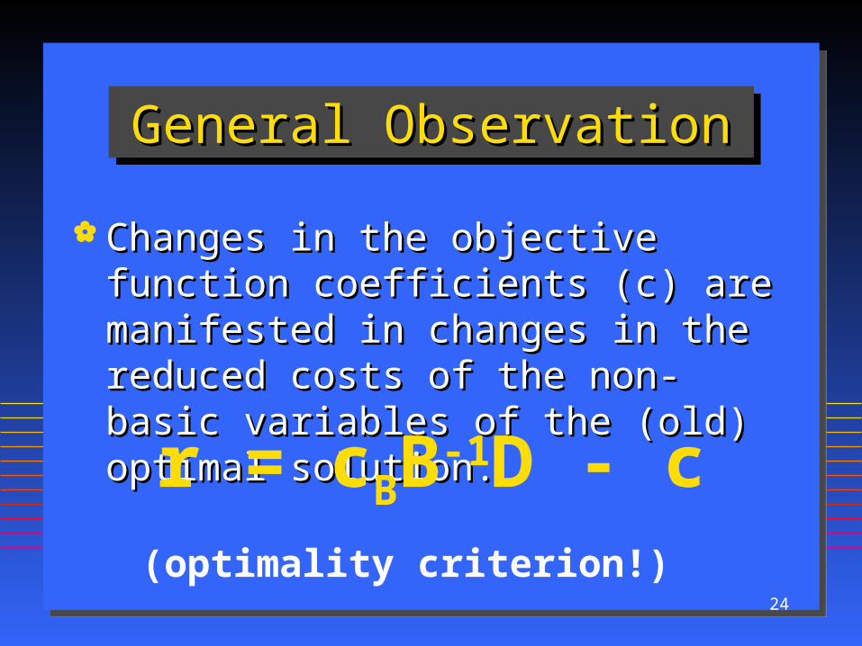
General ObservationGeneral ObservationGeneral ObservationGeneral Observation

Changes in the objective function Changes in the objective function coefficients (c) are manifested in changes in coefficients (c) are manifested in changes in the reduced costs of the non-basic variables the reduced costs of the non-basic variables of the (old) optimal solution. of the (old) optimal solution.

r = cBB-1D - c(optimality criterion!)

25

Observation Observation Observation Observation

Changes in vector b are manifested in Changes in vector b are manifested in changes in the RHS values of the final changes in the RHS values of the final simplex tableau.simplex tableau.

b’ = B-1 b(feasibility)

26

Structural changes, as well as changes in the coefficient matrix (A), may require restoration of the canonical form of the simplex tableau.

27

In short, ... the tasks areIn short, ... the tasks areIn short, ... the tasks areIn short, ... the tasks are

Checking whether the new RHS values are Checking whether the new RHS values are non-negativenon-negative

Checking the signs of the new reduced costsChecking the signs of the new reduced costs Pivot operations to restore the canonical Pivot operations to restore the canonical

form of the simplex tableauform of the simplex tableau

28

RecipeRecipeRecipeRecipe Given the final tableau of the old solution and Given the final tableau of the old solution and

the changes to the model, compute the new the changes to the model, compute the new tableau.tableau.

If the new tableau is not in a canonical form, If the new tableau is not in a canonical form, restore the canonical form by appropriate pivot restore the canonical form by appropriate pivot operations.operations.

Check, if necessary, that the RHS values are Check, if necessary, that the RHS values are non-negative.non-negative.

Check, if necessary, that the reduced costs are of Check, if necessary, that the reduced costs are of the appropriate sign (non-negative for opt=max, the appropriate sign (non-negative for opt=max, non-positive for opt=min).non-positive for opt=min).

29

Implications ....Implications ....Implications ....Implications ....

to accomplish these tasks we need to be able to quickly compute new RHS and/or reduced costs resulting from the changes in the problem.

30

8.3 Overview8.3 Overview8.3 Overview8.3 Overview The formulas used by the Revised Simplex The formulas used by the Revised Simplex

Method suggest what factors should be under Method suggest what factors should be under consideration when parameters of the LP model consideration when parameters of the LP model changechange

These formulas are constructive in developing These formulas are constructive in developing recipes for sensitivity analysis of a number of recipes for sensitivity analysis of a number of important cases.important cases.

Thus,Thus, read again Chapter 6 ....... ???

31

Case 1: All the components Case 1: All the components of the new RHS are non-of the new RHS are non-

negative.negative.

Case 1: All the components Case 1: All the components of the new RHS are non-of the new RHS are non-

negative.negative. In this case the old optimal solution is still In this case the old optimal solution is still

feasible, namely the changes in the problem feasible, namely the changes in the problem do not have any impact on the feasibility of do not have any impact on the feasibility of the "old" optimal solution. We do not have the "old" optimal solution. We do not have to take any "corrective action" as far as to take any "corrective action" as far as feasibility is concerned.feasibility is concerned.

The The new values of the basic variables are of the basic variables are simply equal to the simply equal to the new values of the RHS.of the RHS.

32

Case 2. At least one of the Case 2. At least one of the components of the new RHS is components of the new RHS is

negative.negative.

Case 2. At least one of the Case 2. At least one of the components of the new RHS is components of the new RHS is

negative.negative. Clearly in this case the "old" optimal solution is Clearly in this case the "old" optimal solution is

no longer feasible, as the non-negativity no longer feasible, as the non-negativity constraint is violated by at least one decision constraint is violated by at least one decision variable.variable.

Thus, in this case the changes in the parameters Thus, in this case the changes in the parameters of the model caused the "old" solution to of the model caused the "old" solution to become infeasible and therefore corrective become infeasible and therefore corrective actions involving actions involving changes in the basis, must be must be taken.taken.

33

Case 3. All the components Case 3. All the components of r satisfy the optimality of r satisfy the optimality

condition.condition.

Case 3. All the components Case 3. All the components of r satisfy the optimality of r satisfy the optimality

condition.condition. Since the optimality conditions are satisfiedSince the optimality conditions are satisfied, ,

(by) the basic variables remain basic, thus the basic variables remain basic, thus no corrective actions are required. no corrective actions are required.

Observe, however, that the value of x may Observe, however, that the value of x may have changed due to changes in the vector have changed due to changes in the vector b.b.

34

Case 4. At least one of the Case 4. At least one of the components of r violates the components of r violates the

optimality conditionsoptimality conditions

Case 4. At least one of the Case 4. At least one of the components of r violates the components of r violates the

optimality conditionsoptimality conditions

Obviously, if we exclude degeneracy Obviously, if we exclude degeneracy (why?), there is a need to changes the basis (why?), there is a need to changes the basis itself.itself.

Thus, the changes in the problem results in a Thus, the changes in the problem results in a new basis.new basis.

35

8.4 Common Cases8.4 Common Cases8.4 Common Cases8.4 Common Cases 8.4.1 Changes in the RHS values, b._ Suppose that we change one of the elements of b,

say bk, by . so that the new b is equal to the old one except that the new value of bk is equal to bk+.

_ In short,_ b(new) = b + ek

_ where ek is the kth column of the identity matrix (i.e. ek=(0,0,...0,1,0,...,0) where the 1 is in the kth position).

36

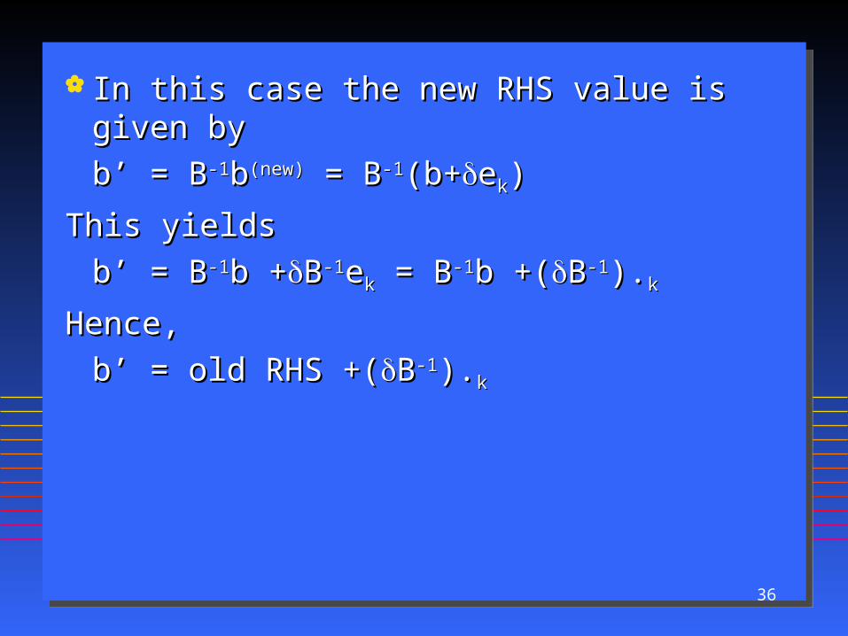
In this case the new RHS value is given byIn this case the new RHS value is given by

b’ = Bb’ = B-1-1bb(new)(new) = B = B-1-1(b+(b+eekk))

This yieldsThis yields

b’ = Bb’ = B-1-1b +b +BB-1-1eekk = B = B-1-1b +(b +(BB-1-1).).kk

Hence,Hence,

b’ = old RHS +(b’ = old RHS +(BB-1-1).).kk

37

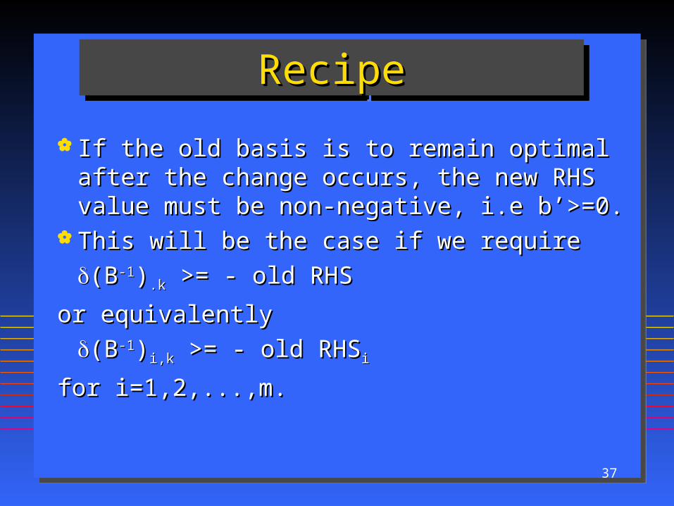
RecipeRecipeRecipeRecipe

If the old basis is to remain optimal after the If the old basis is to remain optimal after the change occurs, the new RHS value must be non-change occurs, the new RHS value must be non-negative, i.e b’>=0.negative, i.e b’>=0.

This will be the case if we requireThis will be the case if we require

(B(B-1-1)).k.k >= - old RHS >= - old RHS

or equivalentlyor equivalently

(B(B-1-1))i,ki,k >= - old RHS >= - old RHSii

for i=1,2,...,m.for i=1,2,...,m.

38

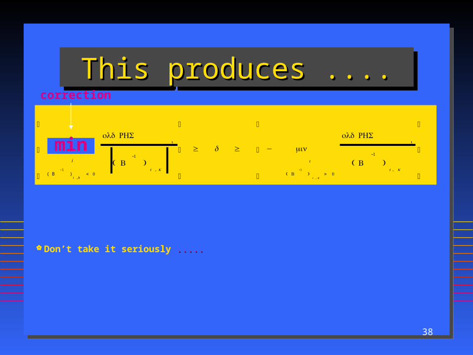
This produces ....This produces ....This produces ....This produces ....

Don’t take it seriously ..........

max

i

( B-1

)i , k

< 0

old RHSi

( B-1

)i , k

⎧

⎨

⎩

⎫

⎬

⎭

≥ ≥ − min i

( B-1

)i , k

> 0

old RHSi

( B-1

)i , k

⎧

⎨

⎩

⎫

⎬

⎭

min

correction

39

8.4.2 Example8.4.2 Example8.4.2 Example8.4.2 Example

b =

48

20

8

⎡

⎣

⎢

⎢

⎤

⎦

⎥

⎥

B

− 1

=

2 4 − 16

0 4 − 8

0 − 1 3

⎡

⎣

⎢

⎢

⎤

⎦

⎥

⎥

k=2

40

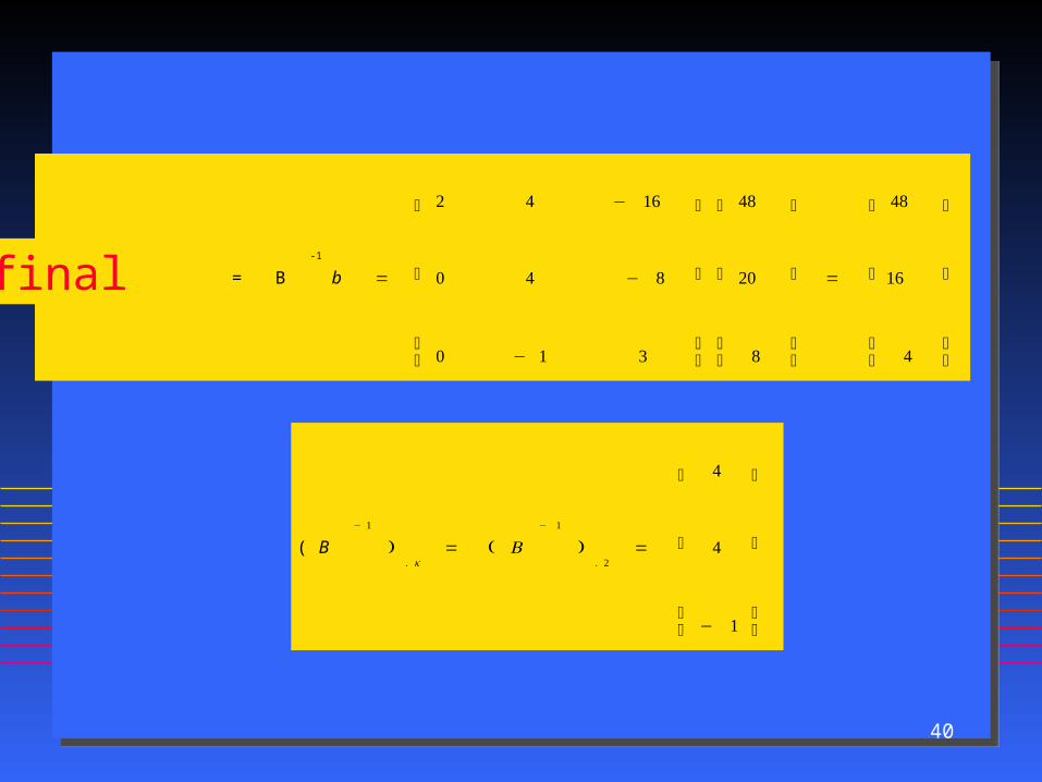
old RHS = B

-1

b =

2 4 − 16

0 4 − 8

0 − 1 3

⎡

⎣

⎢

⎢

⎤

⎦

⎥

⎥

48

20

8

⎡

⎣

⎢

⎢

⎤

⎦

⎥

⎥

=

48

16

4

⎡

⎣

⎢

⎢

⎤

⎦

⎥

⎥

( B

− 1

). k

= ( B− 1

). 2

=

4

4

− 1

⎡

⎣

⎢

⎢

⎤

⎦

⎥

⎥

final

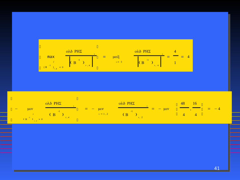
41

max i

( B-1

)i , k

< 0

old RHSi

( B-1

)i , k

⎧

⎨

⎩

⎫

⎬

⎭

= maxi = 3

old RHSi

( B-1

)i , k

=4

1= 4

− min i

( B-1

)i , k

> 0

old RHSi

( B-1

)i , k

⎧

⎨

⎩

⎫

⎬

⎭

= − mini = 1 , 2

old RHSi

( B-1

)i , 2

= − min48

4,16

4

⎧ ⎨ ⎩

⎫ ⎬ ⎭= − 4

42

We therefore conclude that the old basis We therefore conclude that the old basis (whatever it is), will remain optimal if the (whatever it is), will remain optimal if the value of bvalue of b22 is in the interval [20- is in the interval [20-

4,20+4]=[16,24].4,20+4]=[16,24]. Comment:

You do not have to use the recipe: Compute the RHS after the change and determine the critical values of .

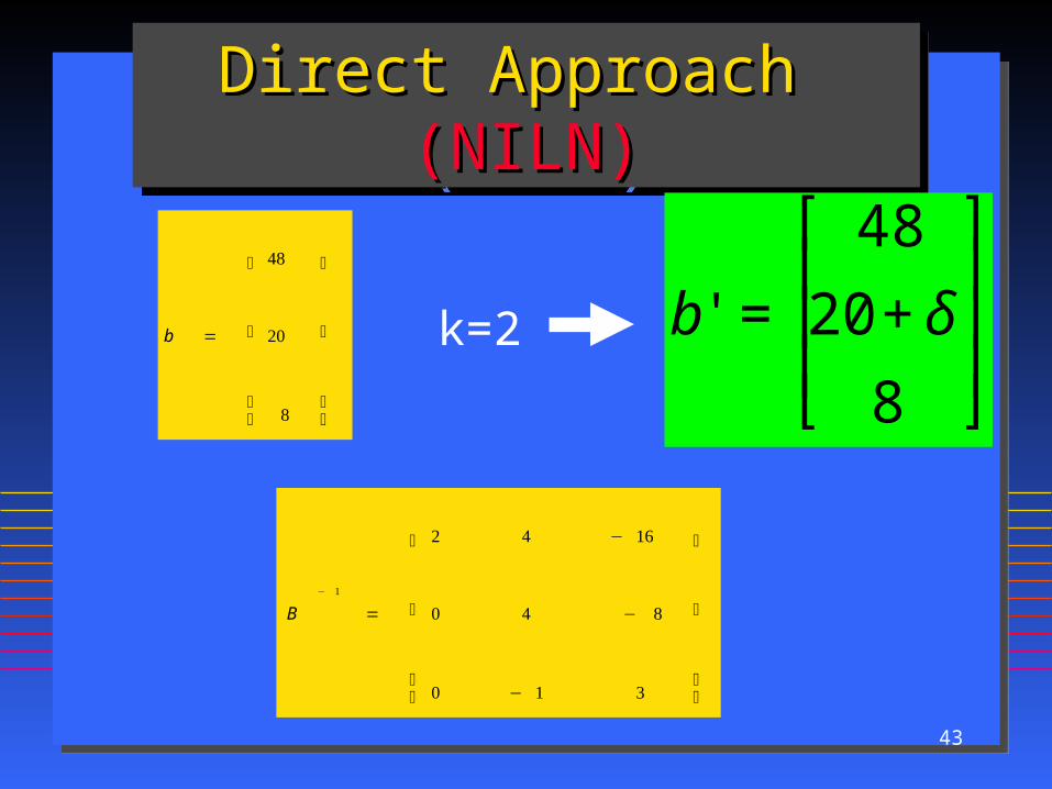
43

Direct ApproachDirect Approach (NILN) (NILN)Direct ApproachDirect Approach (NILN) (NILN)

b =

48

20

8

⎡

⎣

⎢

⎢

⎤

⎦

⎥

⎥

B

− 1

=

2 4 − 16

0 4 − 8

0 − 1 3

⎡

⎣

⎢

⎢

⎤

⎦

⎥

⎥

k=2 b' =

48

20+δ

8

⎡

⎣

⎢ ⎢ ⎢

⎤

⎦

⎥ ⎥ ⎥

44

New final RHS = B-1 b’

new final RHS =

2 4 -16

0 4 −8

0 −1 3

⎡

⎣

⎢ ⎢ ⎢

⎤

⎦

⎥ ⎥ ⎥

48

20+δ

8

⎡

⎣

⎢ ⎢ ⎢

⎤

⎦

⎥ ⎥ ⎥

= ( 96 + 80 + 4 δ − 128 , 80 + 4 δ − 64 , − 20 − δ + 24 )

= ( 48 + 4 δ , 16 + 4 δ , 4 − δ )

45

Thus, the non-negativity constraint requires Thus, the non-negativity constraint requires

48+448+4 >= 0 , hence >= 0 , hence >= -12 >= -12

16+416+4 >= 0 , hence >= 0 , hence >= - 4 >= - 4

4 - 4 - >= 0 , hence >= 0 , hence <= 4 <= 4

In short, In short,

-4 <= -4 <= <= 4 <= 4

(16 <= b(16 <= b22 <= 24) <= 24)

46

8.4.3 Changes in the 8.4.3 Changes in the elements of the cost vector, elements of the cost vector,

c.c.

8.4.3 Changes in the 8.4.3 Changes in the elements of the cost vector, elements of the cost vector,

c.c. Suppose that the value of cSuppose that the value of ckk changes for some k. changes for some k.

How will this affect the optimal solution to the How will this affect the optimal solution to the LP problem?LP problem?

We can distinguish between two cases: We can distinguish between two cases:

(1) x(1) xkk is not in the old basis is not in the old basis

(2) x(2) xkk is in the old basis is in the old basis

rj cB B 1D. j cj , j 1,2, .. .,n

47

Case 1: xCase 1: xkk is not in the old is not in the old

basisbasis

Case 1: xCase 1: xkk is not in the old is not in the old

basisbasis

ThusThus

Recipe::

rrkk >= >= , if opt=max , if opt=max

rrkk <= <= , if opt = min , if opt = min

r'k cBB1D. k (ck ) (cB B

1D. k c ) rk

48

Case 2: xCase 2: xkk is in the old basis is in the old basisCase 2: xCase 2: xkk is in the old basis is in the old basis

c 'B

= cB

+ ep

r ' = c 'B

B

− 1

D − c ' = ( cB

+ δ ep

) B

− 1

D − ( c + δ ek

)

= cBB

− 1

D − c + δ ( epB

− 1

D − ek

)

= r + δ ( epB

− 1

D − ek

)

r ' = r + δ ( t

p •− e

k)

t

p •: = e

pB

− 1

D

49

ObservationsObservationsObservationsObservations

r’r’jj = 0 for basic variables x = 0 for basic variables x jj..

(e(ekk))jj = 0 for all nonbasic variables x = 0 for all nonbasic variables x jj..

if opt=max all the old reduced costs are if opt=max all the old reduced costs are non-negativenon-negative

if opt=min all the old reduced costs are non-if opt=min all the old reduced costs are non-positive.positive.

50

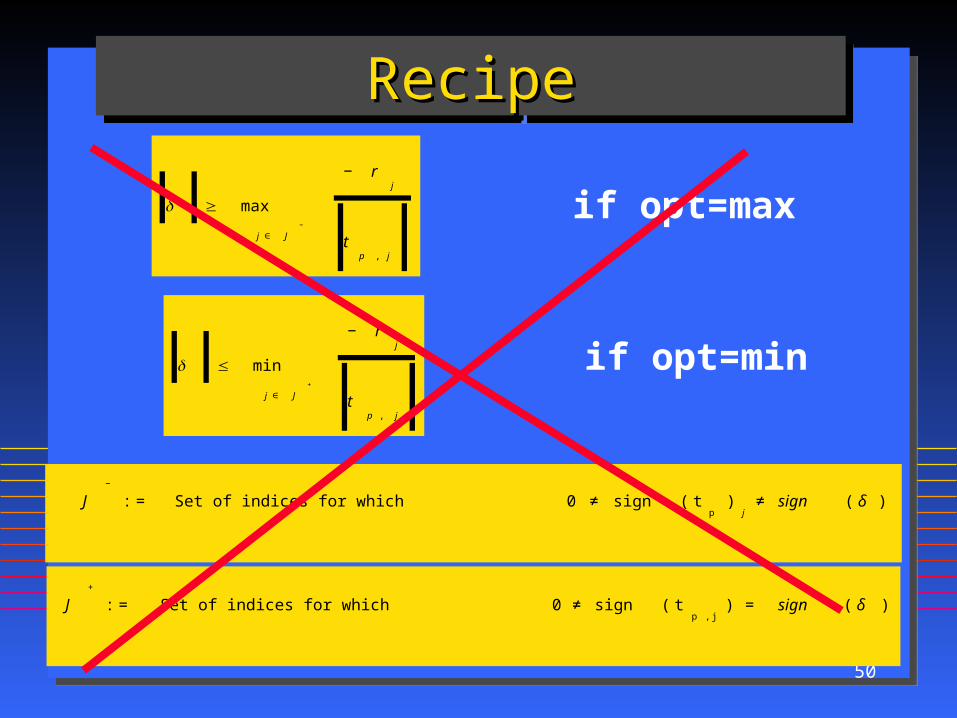
RecipeRecipeRecipeRecipe

≥ max

j ∈ J−

− rj

tp , j

≤ min

j ∈ J+

− rj

tp , j

if opt=max

if opt=min

≥ max

j ∈ J−

− rj

tp , j

J−

: = Set of indices for which 0 ≠ sign ( tp

)j

≠ sign ( δ )

≤ min

j ∈ J+

− rj

tp , j

J+

: = Set of indices for which 0 ≠ sign ( tp , j

) = sign ( δ )

51

RemarkRemarkRemarkRemark

It is very unfortunate that sometime (often?) mathematical notation tends to obscure the essential elements of the situation under investigation. This is a typical example!

As an exercise (on your own) try to translate this to the language of the simplex tableau

52

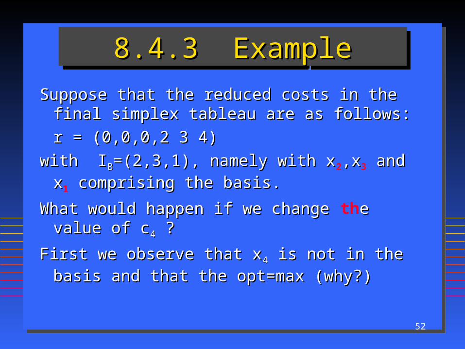
8.4.3 Example8.4.3 Example8.4.3 Example8.4.3 Example

Suppose that the reduced costs in the final simplex Suppose that the reduced costs in the final simplex tableau are as follows:tableau are as follows:

r = (0,0,0,2 3 4)r = (0,0,0,2 3 4)

with Iwith IBB=(2,3,1), namely with x=(2,3,1), namely with x2,x,x3 and x and x1

comprising the basis.comprising the basis.

What would happen if we change What would happen if we change the value of ce value of c44 ? ?

First we observe that xFirst we observe that x44 is not in the basis and that is not in the basis and that

the opt=max (why?) the opt=max (why?)

53

The recipe for this case, namely (8.20) is The recipe for this case, namely (8.20) is that the old optimal solution remains that the old optimal solution remains optimal as long as roptimal as long as r44 ≥ ≥ , or in our case, 2 ≥ , or in our case, 2 ≥

. . Note that we do not need to know the Note that we do not need to know the

current (old) value of ccurrent (old) value of c4 4 to reach this to reach this

conclusion.conclusion. Next, suppose that consider changes in cNext, suppose that consider changes in c11, ,

recalling that xrecalling that x11 is in the basis. is in the basis.

54

recipe for this case:recipe for this case:recipe for this case:recipe for this case:

However, it will be instructive to apply the However, it will be instructive to apply the basic ideas directly! Let's do it.basic ideas directly! Let's do it.

≥ max

j ∈ J−

− r1

tp , 1

55

Preliminary AnalysisPreliminary AnalysisPreliminary AnalysisPreliminary Analysis

We see that in order to analyze this case we We see that in order to analyze this case we have to know the entries in the row of the final have to know the entries in the row of the final tableau (ttableau (tp. p. ) that is represented by x) that is represented by x11 in the in the

basis.basis. What is the value of p?What is the value of p? Since ISince IBB=(2,3,1), this is row p=3.=(2,3,1), this is row p=3.

Suppose that this row is as follows:Suppose that this row is as follows: tt3.3. = (0,0,1,3,-4,0) = (0,0,1,3,-4,0)

56

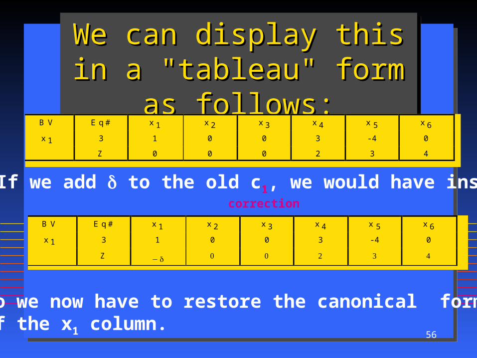
We can display this in a We can display this in a "tableau" form as follows:"tableau" form as follows:We can display this in a We can display this in a

"tableau" form as follows:"tableau" form as follows:B V E q # x 1 x 2 x 3 x 4 x 5 x 6

x 1 3 1 0 0 3 - 4 0

Z 0 0 0 2 3 4

If we add to the old c1, we would have instead

B V E q # x 1 x 2 x 3 x 4 x 5 x 6

x 1 3 1 0 0 3 - 4 0

Z − 0 0 2 3 4

So we now have to restore the canonical form of the x1 column.

correction

57

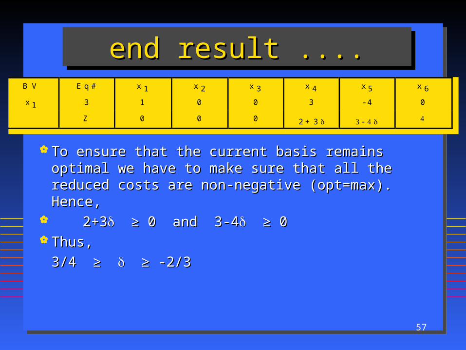
end result ....end result ....end result ....end result ....

To ensure that the current basis remains optimal we To ensure that the current basis remains optimal we have to make sure that all the reduced costs are non-have to make sure that all the reduced costs are non-negative (opt=max). Hence,negative (opt=max). Hence,

2+32+3 ≥ 0 and 3-4 ≥ 0 and 3-4 ≥ 0 ≥ 0 Thus,Thus,

3/4 ≥ 3/4 ≥ ≥ -2/3 ≥ -2/3

B V E q # x 1 x 2 x 3 x 4 x 5 x 6

x 1 3 1 0 0 3 - 4 0

Z 0 0 0 2 + 3 3 - 4 4

58

in words, ....in words, ....in words, ....in words, ....

the old optimal solution will remain optimal the old optimal solution will remain optimal if we keep the increase in cif we keep the increase in c11 in the interval in the interval

[-2/3, 3/4]. If [-2/3, 3/4]. If is too small it will be better is too small it will be better to enter xto enter x44 into the basis, if into the basis, if is too large it is too large it

will better to put xwill better to put x55 into the basis. into the basis.

59

It is strongly recommended that you consider the following structural change on your own:

A new decision variable is introduced. Its cost coefficient is given and its constraint coefficients are given.

How does this affect the given final tableau of the old problem?

60

Warning

If you are asked about the range of admissible changes in say b1 then it is not sufficient to report on the admissible changes in 1 . That is, you have to translate the range of admissible changes in 1 into the range of admissible changes in b1.

Example: Suppose that b1 = 12, and -2 <= 1 <= 3. Then the admissible range of b1 is [12-2 , 12+3 ] = [10,15].