1

Ch. 6: What to Produce?

Where we’ve been… How much to produce? (Ch. 4)

“Factor-product” decision rules say increase production until the marginal cost from an extra unit of output equals the marginal benefit.

How to produce? (Ch. 5)With a least cost combination of inputs.“Factor-factor” decision rules say maintain production, but replace one input for another until the cost of a replaced input equals the cost of adding another input.

2

Ch. 6: What to Produce?NOT on Exam 1, but fair game for FINAL

Where we’re going…Now we add additional types of outputs.

Before: Now:milk milk and cheesePB Cups Reg. and Crunchy PB Cupssweet corn sweet corn and tomatoes

Now there are competing “ends” for our limited resources.(Think opportunity costs.)

Today’s Goals: Two new tools, and a decision rule

3

Assumptions

1. The firm produces two outputs.(a complication)

2. The firm has a fixed set of resources.(a simplification)

3. The firm is a price taker (both in inputs and outputs).

4

Production Possibilities Frontier (PPF)

Ch. 6 Tool #1

The Production Possibilities Frontier (PPF) is a curve depicting all the combinations of two products than can be produced using a given level of inputs.

Sometimes called the production possibilities curve (PPC).

5

Deriving the Production Possibilities Frontier

A Farmers Market Example:

Before, we examined a farmer who was just growing and selling sweet corn.Now we want to expand operations to include tomatoes.

Inputs: Fertilizer, equipment, seed, and other inputs –

These are already purchased, so they’re fixed. Labor – I can hire additional labor, so labor is

variable FOR NOW.

6

Labor Corn Labor Tomatoes

(X) Y 1 (X) Y 2

0 0 0 01 30 1 202 55 2 353 75 3 484 90 4 605 102 5 696 111 6 777 118 7 838 123 8 899 125 9 9410 126 10 98

Two separate production functions for corn (in dozens) and tomatoes (in bushels)

Deriving the Production Possibilities Frontier

What if we contracted for 4 units of labor.

So consider X fixed at 4.

How much corn and tomato production is possible?

7

Labor Corn Labor Tomatoes(X) Y1 (X) Y2

0 0 0 01 30 1 202 55 2 353 75 3 484 90 4 605 102 5 696 111 6 777 118 7 838 123 8 899 125 9 9410 126 10 98

Production combinations for X = 4

X inY 1 X in Y 2 Total X Y 1 Y 2

4 0 4 90 03 1 4 75 202 2 4 55 351 3 4 30 480 4 4 0 60

Deriving the Production Possibilities Frontier

What if we fixed labor at X = 8

8

Deriving the Production Possibilities Frontier

Production combinations for X = 8

X inY 1 X in Y 2 Total X Y 1 Y 2

4 0 4 90 03 1 4 75 202 2 4 55 351 3 4 30 480 4 4 0 60

X inY 1 X in Y 2 Total X Y 1 Y 2

8 0 8 123 07 1 8 118 206 2 8 111 355 3 8 102 484 4 8 90 603 5 8 75 692 6 8 55 771 7 8 30 830 8 8 0 89

Labor Corn Labor Tomatoes(X) Y1 (X) Y2

0 0 0 01 30 1 202 55 2 353 75 3 484 90 4 605 102 5 696 111 6 777 118 7 838 123 8 899 125 9 9410 126 10 98

Let’s graph the PPF when X = 4

9

Deriving the Production Possibilities Frontier (Graphically)

0

20

40

60

80

100

120

140

0 20 40 60 80 100

Tomatoes (Y2)

Cor

n (Y

1)

PPF: X = 4

Let’s add a PPF when X = 8

10

Deriving the Production Possibilities Frontier (Graphically)

0

20

40

60

80

100

120

140

0 20 40 60 80 100

Tomatoes (Y2)

Cor

n (Y

1)

PPF: X = 4

PPF: X = 8

11

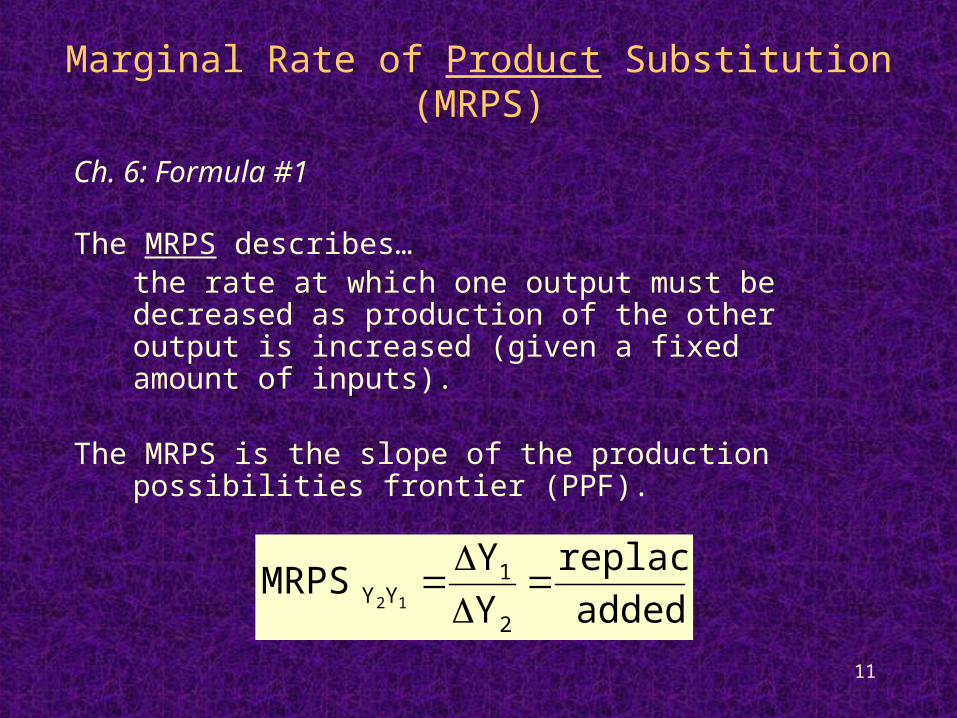
Marginal Rate of Product Substitution (MRPS)

Ch. 6: Formula #1

The MRPS describes…the rate at which one output must be decreased as production of the other output is increased (given a fixed amount of inputs).

The MRPS is the slope of the production possibilities frontier (PPF).

added

replaced

Y

YMRPS

2

1YY 12

12

0

20

40

60

80

100

120

140

0 20 40 60 80 100

Tomatoes (Y2)

Cor

n (Y

1)Marginal Rate of Product Substitution (MRPS)

13

0

20

40

60

80

100

120

140

0 20 40 60 80 100

Tomatoes (Y2)

Cor

n (Y

1)Marginal Rate of Product Substitution (MRPS)

12

12

Y

YMRPS

2

1YY 12

X inY 1 X in Y 2 Total X Y 1 Y 2

8 0 8 123 07 1 8 118 206 2 8 111 355 3 8 102 484 4 8 90 603 5 8 75 692 6 8 55 771 7 8 30 830 8 8 0 89

Any mention of corn or tomato prices yet?

14

Economic Relationships: Isorevenue

Total Revenue:

TR = (PY1 x Y1) + (PY2 x Y2)

Ch.6: Tool #2

Isorevenue line:

A line indicating all combinations of two products that will generate the same level of revenue.

Don’t forget our latest economic “adage”:

Buy low, sell high.

15

Economic Relationships: Isorevenue

Output combinations generating $150 Revenue, where

Price of corn (PY1) = $2.50/dozen

Price of tomatoes (PX2) = $5.00/ bushel

Corn Sold (dozen)

Revenue from Corn

Tomatoes Sold

(bushel)

Revenue from

Tomatoes Total

Y 1 P Y1xY 1 Y 2 P Y2xY 2Revenue

60 150 0 0 15040 100 10 50 15020 50 20 100 1500 0 30 150 150

16

Economic Relationships: Isorevenue

Output combinations generating $150 Revenue with

Price of corn (PY1) = $2.50 and Price of tomatoes (PX2) = $5.00

0

10

20

30

40

50

60

70

80

90

100

110

120

130

140

150

0 10 20 30 40 50 60 70 80

Tomatoes Sold (Y2)

Co

rn S

old

(Y

1)

What happens to the Isorevenue line if we increase our revenue target?

What happens to the line if the price of tomatoes increases?

What happens if the price of tomatoes decreases?

TR=150 TR=225

17

Summary: Isorevenue line

1) The end points show what happens if all production and sales were devoted to a single output.

2) A change in the total revenue is a parallel shift in the isorevenue line.

3) A change in one output price causes the isorevenue line to rotate.

4) The slope of the isorevenue line is also called the “inverse price ratio” (IPR):

Ch. 6: Formula #2

Slope of TR = IPR = -PY2/PY1

18

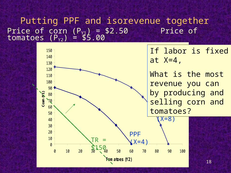
Putting PPF and isorevenue together

0

10

20

30

40

50

60

70

80

90

100

110

120

130

140

150

0 10 20 30 40 50 60 70 80 90 100

Tomatoes (Y2)

Cor

n (Y

1)

PPF (X=4)

PPF (X=8)

TR = $150

Price of corn (PY1) = $2.50 Price of tomatoes (PY2) = $5.00

If labor is fixed at X=4,

What is the most revenue you can by producing and selling corn and tomatoes?

19

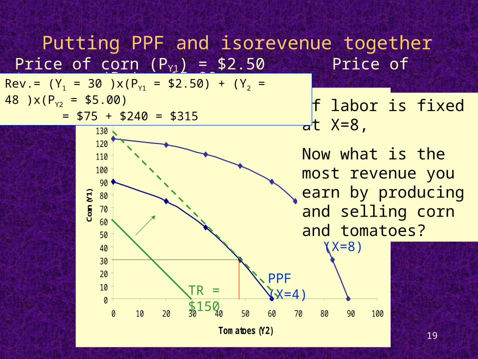
Putting PPF and isorevenue together

0

10

20

30

40

50

60

70

80

90

100

110

120

130

140

150

0 10 20 30 40 50 60 70 80 90 100

Tomatoes (Y2)

Cor

n (Y

1)

PPF (X=4)

PPF (X=8)

TR = $150

If labor is fixed at X=8,

Now what is the most revenue you earn by producing and selling corn and tomatoes?

Price of corn (PY1) = $2.50 Price of tomatoes (PY2) = $5.00Rev.= (Y1 = 30 )x(PY1 = $2.50) + (Y2 = 48 )x(PY2 = $5.00) = $75 + $240 = $315

20

Putting PPF and isorevenue together

0

10

20

30

40

50

60

70

80

90

100

110

120

130

140

150

0 10 20 30 40 50 60 70 80 90 100

Tomatoes (Y2)

Cor

n (Y

1)

PPF (X=4)

PPF (X=8)

TR = $150

Price of corn (PY1) = $2.50 Price of tomatoes (PY2) = $5.00

Rev.= (Y1 = 75 )x(PY1 = $2.50) + (Y2 = 69 )x(PY2 = $5.00) = $187.50 + $345 = $532.50

21

The Decision Rule:

0

10

20

30

40

50

60

70

80

90

100

110

120

130

140

150

0 10 20 30 40 50 60 70 80 90 100

Tomatoes (Y2)

Cor

n (Y

1)

PPF (X=4)

PPF (X=8)

TR = $150

Choose the outputs (Y1 and Y2) so that the slope of the Production Possibility Frontier (PPF) equals the slope of the Isorevenue Line.

1

2

2

112

Y

YYY P

P

Y

YMRPS