1 ch 2.1: linear equations; method of integrating factors a linear first order ode has the general...
Post on 20-Dec-2015
214 views
TRANSCRIPT

1
Ch 2.1: Linear Equations; Method of Integrating Factors
A linear first order ODE has the general form
where f is linear in y. Examples include equations with constant coefficients, such as those in Chapter 1,
or equations with variable coefficients:
),( ytfdt
dy
)()( tgytpdt
dy
bayy

2
Constant Coefficient Case
For a first order linear equation with constant coefficients,
recall that we can use methods of calculus to solve:
Cat ekkeaby
Ctaaby
dtaaby
dy
aaby
dtdy
,/
/ln
/
/
/
,bayy

3
Variable Coefficient Case: Method of Integrating Factors
We next consider linear first order ODEs with variable coefficients:
The method of integrating factors involves multiplying this equation by a function (t), chosen so that the resulting equation is easily integrated.
)()( tgytpdt
dy

4
Example 1: Integrating Factor (1 of 2)
Consider the following equation:
Multiplying both sides by (t), we obtain
We will choose (t) so that left side is derivative of known quantity. Consider the following, and recall product rule:
Choose (t) so that
2/2 teyy
ydt
td
dt
dytyt
dt
d )()()(
tettt 2)()(2)(
)()(2)( 2/ teytdt
dyt t

5
Example 1: General Solution (2 of 2)
With (t) = e2t, we solve the original equation as follows:
tt
tt
tt
ttt
t
t
Ceey
Ceye
eyedt
d
eyedt
dye
etytdt
dyt
eyy
22/
2/52
2/52
2/522
2/
2/
5
25
2
2
)()(2)(
2

6
Method of Integrating Factors: Variable Right Side
In general, for variable right side g(t), the solution can be found as follows:
atatat
atat
atat
atatat
Cedttgeey
dttgeye
tgeyedt
d
tgeyaedt
dye
tgtytadt
dyt
tgayy
)(
)(
)(
)(
)()()()(
)(

7
Example 2: General Solution (1 of 2)
We can solve the following equation
using the formula derived on the previous slide:
Integrating by parts,
Thus
tyy 55
1
5/5/5/ )5()( tttatatat CedtteeCedttgeey
5/5/
5/5/5/
5/5/5/
550
5525
5)5(
tt
ttt
ttt
tee
dtetee
dttedtedtte
5/5/5/5/5/ 550550 ttttt CetCeteeey

8
Example 2: Graphs of Solutions (2 of 2)
The graph on left shows direction field along with several integral curves.
The graph on right shows several solutions, and a particular solution (in red) whose graph contains the point (0,50).
5/55055
1 tCetytyy
9
Example 3: General Solution (1 of 2)
We can solve the following equation
using the formula derived on previous slide:
Integrating by parts,
Thus
tyy 55
1
5/5/5/ )5()( tttatatat CedtteeCedttgeey
5/
5/5/5/
5/5/5/
5
5525
5)5(
t
ttt
ttt
te
dtetee
dttedtedtte
5/5/5/5/ 55 tttt CetCeteey

10
Example 3: Graphs of Solutions (2 of 2)
The graph on left shows direction field along with several integral curves.
The graph on right shows several integral curves, and a particular solution (in red) whose initial point on y-axis separates solutions that grow large positively from those that grow large negatively as t .
5/555/ tCetytyy

11
Method of Integrating Factors for General First Order Linear Equation
Next, we consider the general first order linear equation
Multiplying both sides by (t), we obtain
Next, we want (t) such that '(t) = p(t)(t), from which it will follow that
)()( tgytpy
yttpdt
dytyt
dt
d)()()()(
)()()()()( ttgyttpdt
dyt

12
Integrating Factor for General First Order Linear Equation
Thus we want to choose (t) such that '(t) = p(t)(t).
Assuming (t) > 0, it follows that
Choosing k = 0, we then have
and note (t) > 0 as desired.
ktdtpttdtpt
td )()(ln)(
)(
)(
,)( )( tdtpet

13
Solution forGeneral First Order Linear Equation
Thus we have the following:
Then
tdtpettgtyttpdt
dyt
tgytpy
)()( where),()()()()(
)()(
tdtpett
cdttgty
cdttgtyt
tgtytdt
d
)()( where,)(
)()(
)()()(
)()()(

14
Example 4: General Solution (1 of 3)
To solve the initial value problem
first put into standard form:
Then
and hence
,21,52 2 ytyyt
0for ,52
ttyt
y
222
2
2
ln55
1
51
)(
)()(CtttCdt
tt
t
Ctdtt
t
Cdttgty
2
1ln
ln22
)( 1)(
2
teeeet ttdt
tdttp

15
Example 4: Particular Solution (2 of 3)
Using the initial condition y(1) = 2 and general solution
it follows that
or equivalently,
22 2ln52)1( tttyCy
,ln5 22 Cttty
5/2ln5 2 tty

16
Example 4: Graphs of Solution (3 of 3)
The graphs below show several integral curves for the differential equation, and a particular solution (in red) whose graph contains the initial point (1,2).
22
22
2
2ln5 :Solution Particular
ln5 :Solution General
21,52 :IVP
ttty
Cttty
ytyyt

17
Ch 2.2: Separable Equations
In this section we examine a subclass of linear and nonlinear first order equations. Consider the first order equation
We can rewrite this in the form
For example, let M(x,y) = - f (x,y) and N (x,y) = 1. There may be other ways as well. In differential form,
If M is a function of x only and N is a function of y only, then
In this case, the equation is called separable.
0),(),( dx
dyyxNyxM
0),(),( dyyxNdxyxM
0)()( dyyNdxxM
),( yxfdx
dy

18
Example 1: Solving a Separable Equation
Solve the following first order nonlinear equation:
Separating variables, and using calculus, we obtain
The equation above defines the solution y implicitly. A graph showing the direction field and implicit plots of several integral curves for the differential equation is given above.
1
12
2
y
x
dx
dy
Cxxyy
Cxxyy
dxxdyy
dxxdyy
33
3
1
3
1
11
11
33
33
22
22

19
Example 2: Implicit and Explicit Solutions (1 of 4)
Solve the following first order nonlinear equation:
Separating variables and using calculus, we obtain
The equation above defines the solution y implicitly. An explicit expression for the solution can be found in this case:
12
243 2
y
xx
dx
dy
Cxxxyy
dxxxdyy
dxxxdyy
222
24312
24312
232
2
2
Cxxxy
CxxxyCxxxyy
221
2
224420222
23
23232
20
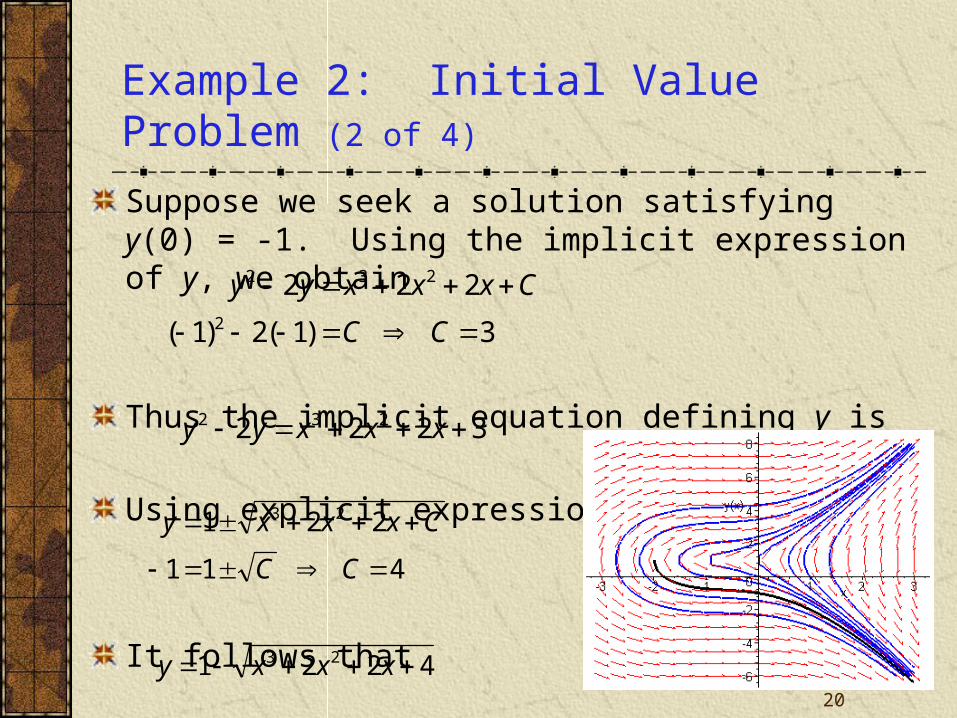
Example 2: Initial Value Problem (2 of 4)
Suppose we seek a solution satisfying y(0) = -1. Using the implicit expression of y, we obtain
Thus the implicit equation defining y is
Using explicit expression of y,
It follows that
411
221 23
CC
Cxxxy
3)1(2)1(
2222
232
CC
Cxxxyy
3222 232 xxxyy
4221 23 xxxy

21
Example 2: Initial Condition y(0) = 3 (3 of 4)
Note that if initial condition is y(0) = 3, then we choose the positive sign, instead of negative sign, on square root term:
4221 23 xxxy

22
Example 2: Domain (4 of 4)
Thus the solutions to the initial value problem
are given by
From explicit representation of y, it follows that
and hence domain of y is (-2, ). Note x = -2 yields y = 1, which makes denominator of dy/dx zero (vertical tangent).
Conversely, domain of y can be estimated by locating vertical tangents on graph (useful for implicitly defined solutions).
(explicit) 4221
(implicit) 3222
23
232
xxxy
xxxyy
2212221 22 xxxxxy
1)0(,12
243 2
yy
xx
dx
dy
23
Example 3: Implicit Solution of Initial Value Problem (1 of 2)
Consider the following initial value problem:
Separating variables and using calculus, we obtain
Using the initial condition, it follows that
1)0(,31
cos3
yy
xyy
Cxyy
xdxdyyy
xdxdyy
y
sinln
cos31
cos31
3
2
3
1sinln 3 xyy

24
Example 3: Graph of Solutions (2 of 2)
Thus
The graph of this solution (black), along with the graphs of the direction field and several integral curves (blue) for this differential equation, is given below.
1sinln1)0(,31
cos 33
xyyyy
xyy

25
Ch 2.4: Differences Between Linear and Nonlinear Equations
Recall that a first order ODE has the form y' = f (t, y), and is linear if f is linear in y, and nonlinear if f is nonlinear in y. Examples: y' = t y - e
t, y' = t y2. In this section, we will see that first order linear and nonlinear equations differ in a number of ways, including:
The theory describing existence and uniqueness of solutions, and corresponding domains, are different. Solutions to linear equations can be expressed in terms of a general solution, which is not usually the case for nonlinear equations. Linear equations have explicitly defined solutions while nonlinear equations typically do not, and nonlinear equations may or may not have implicitly defined solutions.
For both types of equations, numerical and graphical construction of solutions are important.

26
Theorem 2.4.1
Consider the linear first order initial value problem:
If the functions p and g are continuous on an open interval (, ) containing the point t = t0, then there exists a unique solution y = (t) that satisfies the IVP for each t in (, ).
Proof outline: Use Ch 2.1 discussion and results:
0)0(),()( yytgytpdt
dy
t
tdssp
t
t ett
ydttgty 00
)(0
)( where,)(
)()(

27
Theorem 2.4.2
Consider the nonlinear first order initial value problem:
Suppose f and f/y are continuous on some open rectangle (t, y) (, ) x (, ) containing the point (t0, y0). Then in some interval (t0 - h, t0 + h) (, ) there exists a unique solution y = (t) that satisfies the IVP.Proof discussion: Since there is no general formula for the solution of arbitrary nonlinear first order IVPs, this proof is difficult, and is beyond the scope of this course. It turns out that conditions stated in Thm 2.4.2 are sufficient but not necessary to guarantee existence of a solution, and continuity of f ensures existence but not uniqueness of .
0)0(),,( yyytfdt
dy

28
Example 1: Linear IVP
Recall the initial value problem from Chapter 2.1 slides:
The solution to this initial value problem is defined for
t > 0, the interval on which p(t) = -2/t is continuous.
If the initial condition is y(-1) = 2, then the solution is given by same expression as above, but is defined on t < 0.
In either case, Theorem 2.4.1
guarantees that solution is unique
on corresponding interval.
222 2ln521,52 tttyytyyt

29
Example 2: Nonlinear IVP (1 of 2)
Consider nonlinear initial value problem from Ch 2.2:
The functions f and f/y are given by
and are continuous except on line y = 1.
Thus we can draw an open rectangle about (0, -1) on which f and f/y are continuous, as long as it doesn’t cover y = 1.
How wide is rectangle? Recall solution defined for t > -2, with
,
12
243),(,
12
243),( 2
22
y
xxyx
y
f
y
xxyxf
1)0(,12
243 2
yy
xx
dx
dy
4221 23 xxxy

30
Example 2: Change Initial Condition (2 of 2)
Our nonlinear initial value problem is
with
which are continuous except on line y = 1.
If we change initial condition to y(0) = 1, then Theorem 2.4.2 is not satisfied. Solving this new IVP, we obtain
Thus a solution exists but is not unique.
,
12
243),(,
12
243),( 2
22
y
xxyx
y
f
y
xxyxf
1)0(,12
243 2
yy
xx
dx
dy
0,221 23 xxxxy

31
Example 3: Nonlinear IVP
Consider nonlinear initial value problem
The functions f and f/y are given by
Thus f continuous everywhere, but f/y doesn’t exist at y = 0, and hence Theorem 2.4.2 is not satisfied. Solutions exist but are not unique. Separating variables and solving, we obtain
If initial condition is not on t-axis, then Theorem 2.4.2 does guarantee existence and uniqueness.
3/23/1
3
1),(,),(
yyty
fyytf
00)0(,3/1 tyyy
0,3
2
2
32/3
3/23/1
ttyctydtdyy

32
Example 4: Nonlinear IVP
Consider nonlinear initial value problem
The functions f and f/y are given by
Thus f and f/y are continuous at t = 0, so Thm 2.4.2 guarantees that solutions exist and are unique. Separating variables and solving, we obtain
The solution y(t) is defined on (-, 1). Note that the singularity at t = 1 is not obvious from original IVP statement.
yyty
fyytf 2),(,),( 2
1)0(,2 yyy
ty
ctyctydtdyy
1
1112

33
Interval of Definition: Linear Equations
By Theorem 2.4.1, the solution of a linear initial value problem
exists throughout any interval about t = t0 on which p and g are continuous.
Vertical asymptotes or other discontinuities of solution can only occur at points of discontinuity of p or g.
However, solution may be differentiable at points of discontinuity of p or g. See Chapter 2.1: Example 3 of text.
Compare these comments with Example 1 and with previous linear equations in Chapter 1 and Chapter 2.
0)0(),()( yytgytpy

34
Interval of Definition: Nonlinear Equations
In the nonlinear case, the interval on which a solution exists may be difficult to determine.
The solution y = (t) exists as long as (t,(t)) remains within rectangular region indicated in Theorem 2.4.2. This is what determines the value of h in that theorem. Since (t) is usually not known, it may be impossible to determine this region.
In any case, the interval on which a solution exists may have no simple relationship to the function f in the differential equation y' = f (t, y), in contrast with linear equations.
Furthermore, any singularities in the solution may depend on the initial condition as well as the equation.
Compare these comments to the preceding examples.

35
General Solutions
For a first order linear equation, it is possible to obtain a solution containing one arbitrary constant, from which all solutions follow by specifying values for this constant.
For nonlinear equations, such general solutions may not exist. That is, even though a solution containing an arbitrary constant may be found, there may be other solutions that cannot be obtained by specifying values for this constant.
Consider Example 4: The function y = 0 is a solution of the differential equation, but it cannot be obtained by specifying a value for c in solution found using separation of variables:
ctyy
dt
dy
12

36
Explicit Solutions: Linear Equations
By Theorem 2.4.1, a solution of a linear initial value problem
exists throughout any interval about t = t0 on which p and g are continuous, and this solution is unique.
The solution has an explicit representation,
and can be evaluated at any appropriate value of t, as long as the necessary integrals can be computed.
,)( where,)(
)()(00
)(0
t
tdssp
t
t ett
ydttgty
0)0(),()( yytgytpy

37
Explicit Solution Approximation
For linear first order equations, an explicit representation for the solution can be found, as long as necessary integrals can be solved.
If integrals can’t be solved, then numerical methods are often used to approximate the integrals.
n
kkkk
t
t
dssp
t
t
ttgtdttgt
ett
Cdttgty
t
t
1
)(
)()()()(
)( where,)(
)()(
0
00

38
Implicit Solutions: Nonlinear Equations
For nonlinear equations, explicit representations of solutions may not exist.
As we have seen, it may be possible to obtain an equation which implicitly defines the solution. If equation is simple enough, an explicit representation can sometimes be found.
Otherwise, numerical calculations are necessary in order to determine values of y for given values of t. These values can then be plotted in a sketch of the integral curve.
Recall the following example from
Ch 2.2 slides:
1sinln1)0(,31
cos 33
xyyyy
xyy

39
Direction Fields
In addition to using numerical methods to sketch the integral curve, the nonlinear equation itself can provide enough information to sketch a direction field.
The direction field can often show the qualitative form of solutions, and can help identify regions in the ty-plane where solutions exhibit interesting features that merit more detailed analytical or numerical investigations.
Chapter 2.7 and Chapter 8 focus on numerical methods.

40
Ch 2.5: Autonomous Equations and Population Dynamics
In this section we examine equations of the form y' = f (y), called autonomous equations, where the independent variable t does not appear explicitly.
The main purpose of this section is to learn how geometric methods can be used to obtain qualitative information directly from differential equation without solving it.
Example (Exponential Growth):
Solution:
0, rryy
rteyy 0

41
Logistic Growth
An exponential model y' = ry, with solution y = ert, predicts unlimited growth, with rate r > 0 independent of population.
Assuming instead that growth rate depends on population size, replace r by a function h(y) to obtain y' = h(y)y.
We want to choose growth rate h(y) so thath(y) r when y is small,
h(y) decreases as y grows larger, and
h(y) < 0 when y is sufficiently large.
The simplest such function is h(y) = r – ay, where a > 0.
Our differential equation then becomes
This equation is known as the Verhulst, or logistic, equation.
0,, aryayry
42
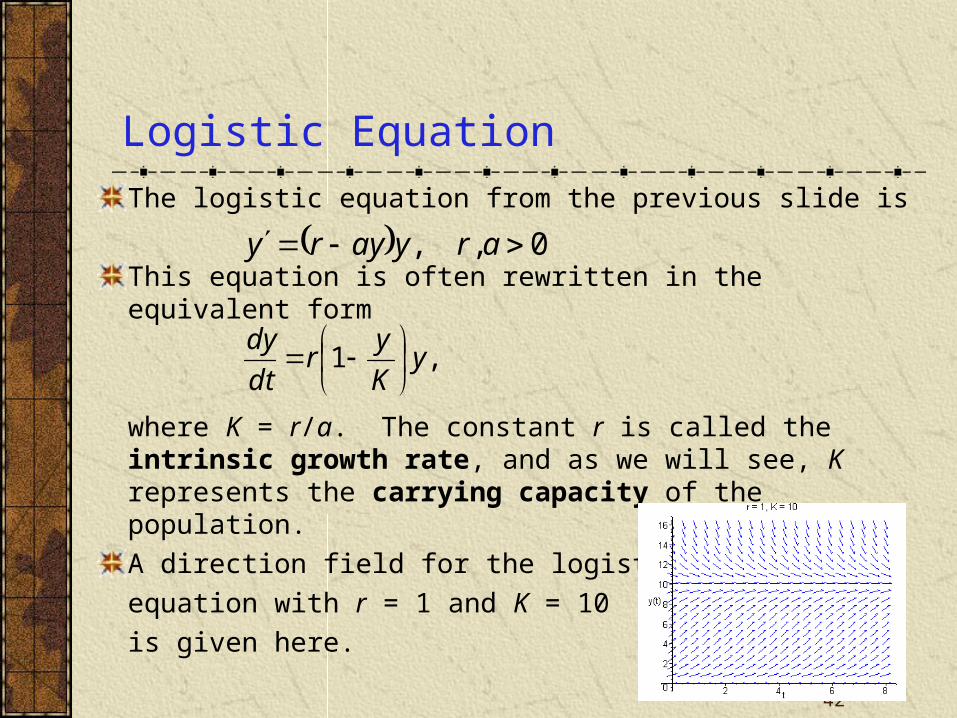
Logistic Equation
The logistic equation from the previous slide is
This equation is often rewritten in the equivalent form
where K = r/a. The constant r is called the intrinsic growth rate, and as we will see, K represents the carrying capacity of the population.
A direction field for the logistic
equation with r = 1 and K = 10
is given here.
,1 yK
yr
dt
dy
0,, aryayry

43
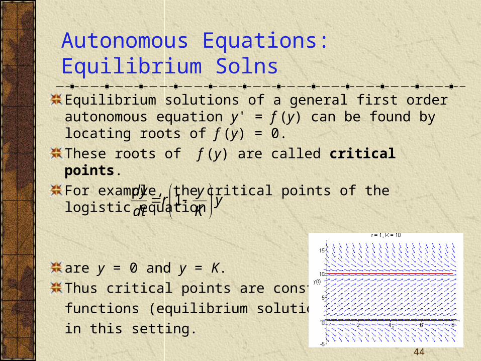
Logistic Equation: Equilibrium Solutions
Our logistic equation is
Two equilibrium solutions are clearly present:
In direction field below, with r = 1, K = 10, note behavior of solutions near equilibrium solutions:
y = 0 is unstable,
y = 10 is asymptotically stable.
0,,1
Kry
K
yr
dt
dy
Ktyty )(,0)( 21
44
Autonomous Equations: Equilibrium Solns
Equilibrium solutions of a general first order autonomous equation y' = f (y) can be found by locating roots of f (y) = 0.
These roots of f (y) are called critical points.
For example, the critical points of the logistic equation
are y = 0 and y = K.
Thus critical points are constant
functions (equilibrium solutions)
in this setting.
yK
yr
dt
dy
1

45
Logistic Equation: Qualitative Analysis and Curve Sketching (1 of 7)
To better understand the nature of solutions to autonomous equations, we start by graphing f (y) vs. y.
In the case of logistic growth, that means graphing the following function and analyzing its graph using calculus.
yK
yryf
1)(

46
Logistic Equation: Critical Points (2 of 7)
The intercepts of f occur at y = 0 and y = K, corresponding to the critical points of logistic equation.
The vertex of the parabola is (K/2, rK/4), as shown below.
4221
2
202
11
)(
1)(
rKK
K
Kr
Kf
KyKy
K
r
K
yy
Kryf
yK
yryf
set

47
Logistic Solution: Increasing, Decreasing (3 of 7)
Note dy/dt > 0 for 0 < y < K, so y is an increasing function of t there (indicate with right arrows along y-axis on 0 < y < K).
Similarly, y is a decreasing function of t for y > K (indicate with left arrows along y-axis on y > K).
In this context the y-axis is often called the phase line.
0,1
ry
K
yr
dt
dy

48
Logistic Solution: Steepness, Flatness (4 of 7)
Note dy/dt 0 when y 0 or y K, so y is relatively flat there, and y gets steep as y moves away from 0 or K.
yK
yr
dt
dy
1

49
Logistic Solution: Concavity (5 of 7)
Next, to examine concavity of y(t), we find y'':
Thus the graph of y is concave up when f and f ' have same sign, which occurs when 0 < y < K/2 and y > K.
The graph of y is concave down when f and f ' have opposite signs, which occurs when K/2 < y < K.
Inflection point occurs at intersection of y and line y = K/2.
)()()()(2
2
yfyfdt
dyyf
dt
ydyf
dt
dy

50
Logistic Solution: Curve Sketching (6 of 7)
Combining the information on the previous slides, we have:Graph of y increasing when 0 < y < K.
Graph of y decreasing when y > K.
Slope of y approximately zero when y 0 or y K.
Graph of y concave up when 0 < y < K/2 and y > K.
Graph of y concave down when K/2 < y < K.
Inflection point when y = K/2.
Using this information, we can
sketch solution curves y for
different initial conditions.

51
Logistic Solution: Discussion (7 of 7)
Using only the information present in the differential equation and without solving it, we obtained qualitative information about the solution y.
For example, we know where the graph of y is the steepest, and hence where y changes most rapidly. Also, y tends asymptotically to the line y = K, for large t.
The value of K is known as the carrying capacity, or saturation level, for the species.
Note how solution behavior differs
from that of exponential equation,
and thus the decisive effect of
nonlinear term in logistic equation.

52
Solving the Logistic Equation (1 of 3)
Provided y 0 and y K, we can rewrite the logistic ODE:
Expanding the left side using partial fractions,
Thus the logistic equation can be rewritten as
Integrating the above result, we obtain
rdtyKy
dy
1
rdtdyKy
K
y
/1
/11
CrtK
yy 1lnln
KyABKyBAyy
B
Ky
A
yKy
,111
11
1

53
Solving the Logistic Equation (2 of 3)
We have:
If 0 < y0 < K, then 0 < y < K and hence
Rewriting, using properties of logs:
CrtK
yy
1lnln
CrtK
yy 1lnln
)0( where,or
111ln
000
0 yyeyKy
Kyy
ceKy
ye
Ky
yCrt
Ky
y
rt
rtCrt

54
Solution of the Logistic Equation (3 of 3)
We have:
for 0 < y0 < K.
It can be shown that solution is also valid for y0 > K. Also, this solution contains equilibrium solutions y = 0 and y = K.
Hence solution to logistic equation is
rteyKy
Kyy
00
0
rteyKy
Kyy
00
0

55
Logistic Solution: Asymptotic Behavior
The solution to logistic ODE is
We use limits to confirm asymptotic behavior of solution:
Thus we can conclude that the equilibrium solution y(t) = K is asymptotically stable, while equilibrium solution y(t) = 0 is unstable. The only way to guarantee solution remains near zero is to make y0 = 0.
rteyKy
Kyy
00
0
Ky
Ky
eyKy
Kyy
trttt
0
0
00
0 limlimlim

56
Example: Pacific Halibut (1 of 2)
Let y be biomass (in kg) of halibut population at time t, with r = 0.71/year and K = 80.5 x 10⁶ kg. If y0 = 0.25K, find
(a) biomass 2 years later
(b) the time such that y() = 0.75K.
(a) For convenience, scale equation:
Then
and hence
rteyKy
Kyy
00
0
rteKyKy
Ky
K
y
00
0
1
5797.075.025.0
25.0)2()2)(71.0(
eK
y
kg 107.465797.0)2( 6 Ky

57
Example: Pacific Halibut, Part (b) (2 of 2)
(b) Find time for which y() = 0.75K.
years 095.375.03
25.0ln
71.0
1
13175.0
25.0
175.075.0
175.0
175.0
0
0
0
0
000
000
00
0
Ky
Ky
Ky
Kye
KyeKyKy
K
ye
K
y
K
y
eKyKy
Ky
r
r
r
r
rteKyKy
Ky
K
y
00
0
1

58
Critical Threshold Equation (1 of 2)
Consider the following modification of the logistic ODE:
The graph of the right hand side f (y) is given below.
0,1
ry
T
yr
dt
dy

59
Critical Threshold Equation: Qualitative Analysis and Solution (2 of 2)
Performing an analysis similar to that of the logistic case, we obtain a graph of solution curves shown below.
T is a threshold value for y0, in that population dies off or grows unbounded, depending on which side of T the initial value y0 is.
See also laminar flow discussion in text.
It can be shown that the solution to the threshold equation
is
0,1
ry
T
yr
dt
dy
rteyTy
Tyy
00
0

60
Logistic Growth with a Threshold (1 of 2)
In order to avoid unbounded growth for y > T as in previous setting, consider the following modification of the logistic equation:
The graph of the right hand side f (y) is given below.
KTryK
y
T
yr
dt
dy
0 and 0,11

61
Logistic Growth with a Threshold (2 of 2)
Performing an analysis similar to that of the logistic case, we obtain a graph of solution curves shown below right.
T is threshold value for y0, in that population dies off or grows towards K, depending on which side of T y0 is.
K is the carrying capacity level.
Note: y = 0 and y = K are stable equilibrium solutions,
and y = T is an unstable equilibrium solution.

62
Ch 2.6: Exact Equations & Integrating Factors
Consider a first order ODE of the form
Suppose there is a function such that
and such that (x,y) = c defines y = (x) implicitly. Then
and hence the original ODE becomes
Thus (x,y) = c defines a solution implicitly. In this case, the ODE is said to be exact.
0),(),( yyxNyxM
),(),(),,(),( yxNyxyxMyx yx
)(,),(),( xxdx
d
dx
dy
yxyyxNyxM
0)(, xxdx
d

63
Suppose an ODE can be written in the form
where the functions M, N, My and Nx are all continuous in the rectangular region R: (x, y) (, ) x (, ). Then Eq. (1) is an exact differential equation iff
That is, there exists a function satisfying the conditions
iff M and N satisfy Equation (2).
)1(0),(),( yyxNyxM
)2(),(),,(),( RyxyxNyxM xy
)3(),(),(),,(),( yxNyxyxMyx yx
Theorem 2.6.1
64
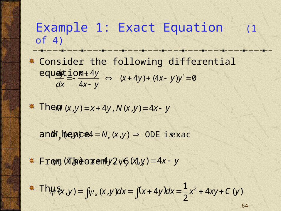
Example 1: Exact Equation (1 of 4)
Consider the following differential equation.
Then
and hence
From Theorem 2.6.1,
Thus
0)4()4(4
4
yyxyxyx
yx
dx
dy
yxyxNyxyxM 4),(,4),(
exact is ODE),(4),( yxNyxM xy
yxyxyxyx yx 4),(,4),(
)(42
14),(),( 2 yCxyxdxyxdxyxyx x

65
Example 1: Solution (2 of 4)
We have
and
It follows that
Thus
By Theorem 2.6.1, the solution is given implicitly by
yxyxyxyx yx 4),(,4),(
)(42
14),(),( 2 yCxyxdxyxdxyxyx x
kyyCyyCyCxyxyxy 2
2
1)()()(44),(
kyxyxyx 22
2
14
2
1),(
cyxyx 22 8

66
Example 1: Direction Field and Solution Curves (3 of 4)
Our differential equation and solutions are given by
A graph of the direction field for this differential equation,
along with several solution curves, is given below.
cyxyxyyxyxyx
yx
dx
dy
22 80)4()4(4
4

67
Example 1: Explicit Solution and Graphs (4 of 4)
Our solution is defined implicitly by the equation below.
In this case, we can solve the equation explicitly for y:
Solution curves for several values of c are given below.
cxxycxxyy 222 17408
cyxyx 22 8

68
Example 2: Exact Equation (1 of 3)
Consider the following differential equation.
Then
and hence
From Theorem 2.6.1,
Thus
0)1(sin)2cos( 2 yexxxexy yy
1sin),(,2cos),( 2 yy exxyxNxexyyxM
exact is ODE),(2cos),( yxNxexyxM xy
y
1sin),(,2cos),( 2 yy
yx exxNyxxexyMyx
)(sin2cos),(),( 2 yCexxydxxexydxyxyx yyx

69
Example 2: Solution (2 of 3)
We have
and
It follows that
Thus
By Theorem 2.6.1, the solution is given implicitly by
1sin),(,2cos),( 2 yy
yx exxNyxxexyMyx
)(sin2cos),(),( 2 yCexxydxxexydxyxyx yyx
kyyCyC
yCexxexxyx yyy
)(1)(
)(sin1sin),( 22
kyexxyyx y 2sin),(
cyexxy y 2sin

70
Example 2: Direction Field and Solution Curves (3 of 3)
Our differential equation and solutions are given by
A graph of the direction field for this differential equation,
along with several solution curves, is given below.
cyexxy
yexxxexyy
yy
2
2
sin
,0)1(sin)2cos(

71
Example 3: Non-Exact Equation (1 of 3)
Consider the following differential equation.
Then
and hence
To show that our differential equation cannot be solved by this method, let us seek a function such that
Thus
0)2()3( 32 yxxyyxy
32 2),(,3),( xxyyxNyxyyxM
exactnot is ODE),(3223),( 2 yxNxyyxyxM xy
32 2),(,3),( xxyNyxyxyMyx yx
)(2/33),(),( 222 yCxyyxdxyxydxyxyx x

72
Example 3: Non-Exact Equation (2 of 3)
We seek such that
and
Then
Thus there is no such function . However, if we (incorrectly) proceed as before, we obtain
as our implicitly defined y, which is not a solution of ODE.
32 2),(,3),( xxyNyxyxyMyx yx
)(2/33),(),( 222 yCxyyxdxyxydxyxyx x
kyxyxyCxxyC
yCxyxxxyyxy
2/3)(2/3)(
)(22/32),(
23??
23?
23
cxyyx 23

73
Example 3: Graphs (3 of 3)
Our differential equation and implicitly defined y are
A plot of the direction field for this differential equation,
along with several graphs of y, are given below.
From these graphs, we see further evidence that y does not satisfy the differential equation.
cxyyx
yxxyyxy
23
32 ,0)2()3(

74
It is sometimes possible to convert a differential equation that is not exact into an exact equation by multiplying the equation by a suitable integrating factor (x, y):
For this equation to be exact, we need
This partial differential equation may be difficult to solve. If is a function of x alone, then y = 0 and hence we solve
provided right side is a function of x only. Similarly if is a function of y alone. See text for more details.
Integrating Factors
0),(),(),(),(
0),(),(
yyxNyxyxMyx
yyxNyxM
0 xyxyxy NMNMNM
,N
NM
dx
d xy

75
Example 4: Non-Exact Equation
Consider the following non-exact differential equation.
Seeking an integrating factor, we solve the linear equation
Multiplying our differential equation by , we obtain the exact equation
which has its solutions given implicitly by
0)()3( 22 yxyxyxy
xxxdx
d
N
NM
dx
d xy
)(
,0)()3( 2322 yyxxxyyx
cyxyx 223
2
1