1 an introduction to conditional random fields for...

1 An Introduction to Conditional Random

Fields for Relational Learning

Charles SuttonDepartment of Computer ScienceUniversity of Massachusetts, [email protected]://www.cs.umass.edu/∼casutton

Andrew McCallumDepartment of Computer ScienceUniversity of Massachusetts, [email protected]://www.cs.umass.edu/∼mccallum

1.1 Introduction

Relational data has two characteristics: first, statistical dependencies exist betweenthe entities we wish to model, and second, each entity often has a rich set of featuresthat can aid classification. For example, when classifying Web documents, thepage’s text provides much information about the class label, but hyperlinks definea relationship between pages that can improve classification [Taskar et al., 2002].Graphical models are a natural formalism for exploiting the dependence structureamong entities. Traditionally, graphical models have been used to represent thejoint probability distribution p(y,x), where the variables y represent the attributesof the entities that we wish to predict, and the input variables x represent ourobserved knowledge about the entities. But modeling the joint distribution canlead to difficulties when using the rich local features that can occur in relationaldata, because it requires modeling the distribution p(x), which can include complexdependencies. Modeling these dependencies among inputs can lead to intractablemodels, but ignoring them can lead to reduced performance.A solution to this problem is to directly model the conditional distribution p(y|x),which is sufficient for classification. This is the approach taken by conditional ran-dom fields [Lafferty et al., 2001]. A conditional random field is simply a conditionaldistribution p(y|x) with an associated graphical structure. Because the model is

2 An Introduction to Conditional Random Fields for Relational Learning

conditional, dependencies among the input variables x do not need to be explicitlyrepresented, affording the use of rich, global features of the input. For example,in natural language tasks, useful features include neighboring words and word bi-grams, prefixes and suffixes, capitalization, membership in domain-specific lexicons,and semantic information from sources such as WordNet. Recently there has beenan explosion of interest in CRFs, with successful applications including text process-ing [Taskar et al., 2002, Peng and McCallum, 2004, Settles, 2005, Sha and Pereira,2003], bioinformatics [Sato and Sakakibara, 2005, Liu et al., 2005], and computervision [He et al., 2004, Kumar and Hebert, 2003].This chapter is divided into two parts. First, we present a tutorial on currenttraining and inference techniques for conditional random fields. We discuss theimportant special case of linear-chain CRFs, and then we generalize these toarbitrary graphical structures. We include a brief discussion of techniques forpractical CRF implementations.Second, we present an example of applying a general CRF to a practical relationallearning problem. In particular, we discuss the problem of information extraction,that is, automatically building a relational database from information containedin unstructured text. Unlike linear-chain models, general CRFs can capture longdistance dependencies between labels. For example, if the same name is mentionedmore than once in a document, all mentions probably have the same label, and itis useful to extract them all, because each mention may contain different comple-mentary information about the underlying entity. To represent these long-distancedependencies, we propose a skip-chain CRF, a model that jointly performs seg-mentation and collective labeling of extracted mentions. On a standard problemof extracting speaker names from seminar announcements, the skip-chain CRF hasbetter performance than a linear-chain CRF.

1.2 Graphical Models

1.2.1 Definitions

We consider probability distributions over sets of random variables V = X ∪ Y ,where X is a set of input variables that we assume are observed, and Y is a set ofoutput variables that we wish to predict. Every variable v ∈ V takes outcomes froma set V, which can be either continuous or discrete, although we discuss only thediscrete case in this chapter. We denote an assignment to X by x, and we denotean assignment to a set A ⊂ X by xA, and similarly for Y . We use the notation1{x=x′} to denote an indicator function of x which takes the value 1 when x = x′

and 0 otherwise.A graphical model is a family of probability distributions that factorize accordingto an underlying graph. The main idea is to represent a distribution over a largenumber of random variables by a product of local functions that each depend ononly a small number of variables. Given a collection of subsets A ⊂ V , we define

1.2 Graphical Models 3

an undirected graphical model as the set of all distributions that can be written inthe form

p(x,y) =1Z

∏A

ΨA(xA,yA), (1.1)

for any choice of factors F = {ΨA}, where ΨA : Vn → <+. (These functions arealso called local functions or compatibility functions.) We will occasionally use theterm random field to refer to a particular distribution among those defined by anundirected model. To reiterate, we will consistently use the term model to refer to afamily of distributions, and random field (or more commonly, distribution) to referto a single one.The constant Z is a normalization factor defined as

Z =∑x,y

∏A

ΨA(xA,yA), (1.2)

which ensures that the distribution sums to 1. The quantity Z, considered as afunction of the set F of factors, is called the partition function in the statisticalphysics and graphical models communities. Computing Z is intractable in general,but much work exists on how to approximate it.Graphically, we represent the factorization (1.1) by a factor graph [Kschischanget al., 2001]. A factor graph is a bipartite graph G = (V, F,E) in which a variablenode vs ∈ V is connected to a factor node ΨA ∈ F if vs is an argument to ΨA. Anexample of a factor graph is shown graphically in Figure 1.1 (right). In that figure,the circles are variable nodes, and the shaded boxes are factor nodes.In this chapter, we will assume that each local function has the form

ΨA(xA,yA) = exp

{∑k

θAkfAk(xA,yA)

}, (1.3)

for some real-valued parameter vector θA, and for some set of feature functions orsufficient statistics {fAk}. This form ensures that the family of distributions over V

parameterized by θ is an exponential family. Much of the discussion in this chapteractually applies to exponential families in general.A directed graphical model, also known as a Bayesian network, is based on a directedgraph G = (V,E). A directed model is a family of distributions that factorize as:

p(y,x) =∏v∈V

p(v|π(v)), (1.4)

where π(v) are the parents of v in G. An example of a directed model is shown inFigure 1.1 (left).We use the term generative model to refer to a directed graphical model in whichthe outputs topologically precede the inputs, that is, no x ∈ X can be a parent ofan output y ∈ Y . Essentially, a generative model is one that directly describes howthe outputs probabilistically “generate” the inputs.


x

y

x

y

Figure 1.1 The naive Bayes classifier, as a directed model (left), and as a factorgraph (right).

1.2.2 Applications of graphical models

In this section we discuss a few applications of graphical models to natural languageprocessing. Although these examples are well-known, they serve both to clarify thedefinitions in the previous section, and to illustrate some ideas that will arise againin our discussion of conditional random fields. We devote special attention to thehidden Markov model (HMM), because it is closely related to the linear-chain CRF.

1.2.2.1 Classification

First we discuss the problem of classification, that is, predicting a single classvariable y given a vector of features x = (x1, x2, . . . , xK). One simple way toaccomplish this is to assume that once the class label is known, all the featuresare independent. The resulting classifier is called the naive Bayes classifier. It isbased on a joint probability model of the form:

p(y,x) = p(y)K∏

k=1

p(xk|y). (1.5)

This model can be described by the directed model shown in Figure 1.1 (left). Wecan also write this model as a factor graph, by defining a factor Ψ(y) = p(y), anda factor Ψk(y, xk) = p(xk|y) for each feature xk. This factor graph is shown inFigure 1.1 (right).Another well-known classifier that is naturally represented as a graphical model islogistic regression (sometimes known as the maximum entropy classifier in the NLPcommunity). In statistics, this classifier is motivated by the assumption that the logprobability, log p(y|x), of each class is a linear function of x, plus a normalizationconstant. This leads to the conditional distribution:

p(y|x) =1

Z(x)exp

λy +K∑

j=1

λy,jxj

, (1.6)

where Z(x) =∑

y exp{λy +∑K

j=1 λy,jxj} is a normalizing constant, and λy is abias weight that acts like log p(y) in naive Bayes. Rather than using one vector perclass, as in (1.6), we can use a different notation in which a single set of weights isshared across all the classes. The trick is to define a set of feature functions that are


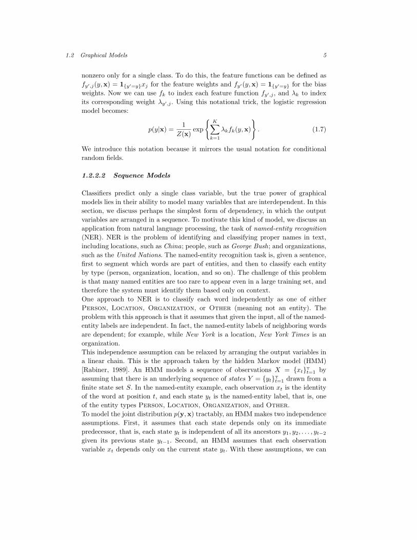
nonzero only for a single class. To do this, the feature functions can be defined asfy′,j(y,x) = 1{y′=y}xj for the feature weights and fy′(y,x) = 1{y′=y} for the biasweights. Now we can use fk to index each feature function fy′,j , and λk to indexits corresponding weight λy′,j . Using this notational trick, the logistic regressionmodel becomes:

p(y|x) =1

Z(x)exp

{K∑

k=1

λkfk(y,x)

}. (1.7)

We introduce this notation because it mirrors the usual notation for conditionalrandom fields.

1.2.2.2 Sequence Models

Classifiers predict only a single class variable, but the true power of graphicalmodels lies in their ability to model many variables that are interdependent. In thissection, we discuss perhaps the simplest form of dependency, in which the outputvariables are arranged in a sequence. To motivate this kind of model, we discuss anapplication from natural language processing, the task of named-entity recognition(NER). NER is the problem of identifying and classifying proper names in text,including locations, such as China; people, such as George Bush; and organizations,such as the United Nations. The named-entity recognition task is, given a sentence,first to segment which words are part of entities, and then to classify each entityby type (person, organization, location, and so on). The challenge of this problemis that many named entities are too rare to appear even in a large training set, andtherefore the system must identify them based only on context.One approach to NER is to classify each word independently as one of eitherPerson, Location, Organization, or Other (meaning not an entity). Theproblem with this approach is that it assumes that given the input, all of the named-entity labels are independent. In fact, the named-entity labels of neighboring wordsare dependent; for example, while New York is a location, New York Times is anorganization.This independence assumption can be relaxed by arranging the output variables ina linear chain. This is the approach taken by the hidden Markov model (HMM)[Rabiner, 1989]. An HMM models a sequence of observations X = {xt}T

t=1 byassuming that there is an underlying sequence of states Y = {yt}T

t=1 drawn from afinite state set S. In the named-entity example, each observation xt is the identityof the word at position t, and each state yt is the named-entity label, that is, oneof the entity types Person, Location, Organization, and Other.To model the joint distribution p(y,x) tractably, an HMM makes two independenceassumptions. First, it assumes that each state depends only on its immediatepredecessor, that is, each state yt is independent of all its ancestors y1, y2, . . . , yt−2

given its previous state yt−1. Second, an HMM assumes that each observationvariable xt depends only on the current state yt. With these assumptions, we can


specify an HMM using three probability distributions: first, the distribution p(y1)over initial states; second, the transition distribution p(yt|yt−1); and finally, theobservation distribution p(xt|yt). That is, the joint probability of a state sequencey and an observation sequence x factorizes as

p(y,x) =T∏

t=1

p(yt|yt−1)p(xt|yt), (1.8)

where, to simplify notation, we write the initial state distribution p(y1) as p(y1|y0).In natural language processing, HMMs have been used for sequence labeling taskssuch as part-of-speech tagging, named-entity recognition, and information extrac-tion.

1.2.3 Discriminative and Generative Models

An important difference between naive Bayes and logistic regression is that naiveBayes is generative, meaning that it is based on a model of the joint distributionp(y,x), while logistic regression is discriminative, meaning that it is based ona model of the conditional distribution p(y|x). In this section, we discuss thedifferences between generative and discriminative modeling, and the advantages ofdiscriminative modeling for many tasks. For concreteness, we focus on the examplesof naive Bayes and logistic regression, but the discussion in this section actuallyapplies in general to the differences between generative models and conditionalrandom fields.The main difference is that a conditional distribution p(y|x) does not include amodel of p(x), which is not needed for classification anyway. The difficulty inmodeling p(x) is that it often contains many highly dependent features, whichare difficult to model. For example, in named-entity recognition, an HMM relies ononly one feature, the word’s identity. But many words, especially proper names, willnot have occurred in the training set, so the word-identity feature is uninformative.To label unseen words, we would like to exploit other features of a word, such asits capitalization, its neighboring words, its prefixes and suffixes, its membership inpredetermined lists of people and locations, and so on.To include interdependent features in a generative model, we have two choices: en-hance the model to represent dependencies among the inputs, or make simplifyingindependence assumptions, such as the naive Bayes assumption. The first approach,enhancing the model, is often difficult to do while retaining tractability. For exam-ple, it is hard to imagine how to model the dependence between the capitalization ofa word and its suffixes, nor do we particularly wish to do so, since we always observethe test sentences anyway. The second approach, adding independence assumptionsamong the inputs, is problematic because it can hurt performance. For example,although the naive Bayes classifier performs surprisingly well in document classi-fication, it performs worse on average across a range of applications than logisticregression [Caruana and Niculescu-Mizil, 2005].


Logistic Regression

HMMs

Linear-chain CRFs

Naive BayesSEQUENCE

SEQUENCE

CONDITIONAL CONDITIONAL

Generative directed models

General CRFs

CONDITIONAL

GeneralGRAPHS

GeneralGRAPHS

Figure 1.2 Diagram of the relationship between naive Bayes, logistic regression,HMMs, linear-chain CRFs, generative models, and general CRFs.

Furthermore, even when naive Bayes has good classification accuracy, its prob-ability estimates tend to be poor. To understand why, imagine training naiveBayes on a data set in which all the features are repeated, that is, x =(x1, x1, x2, x2, . . . , xK , xK). This will increase the confidence of the naive Bayesprobability estimates, even though no new information has been added to the data.Assumptions like naive Bayes can be especially problematic when we generalizeto sequence models, because inference essentially combines evidence from differentparts of the model. If probability estimates at a local level are overconfident, itmight be difficult to combine them sensibly.Actually, the difference in performance between naive Bayes and logistic regressionis due only to the fact that the first is generative and the second discriminative;the two classifiers are, for discrete input, identical in all other respects. Naive Bayesand logistic regression consider the same hypothesis space, in the sense that anylogistic regression classifier can be converted into a naive Bayes classifier with thesame decision boundary, and vice versa. Another way of saying this is that the naiveBayes model (1.5) defines the same family of distributions as the logistic regressionmodel (1.7), if we interpret it generatively as

p(y,x) =exp {

∑k λkfk(y,x)}∑

y,x exp {∑

k λkfk(y, x)}. (1.9)

This means that if the naive Bayes model (1.5) is trained to maximize the con-ditional likelihood, we recover the same classifier as from logistic regression. Con-versely, if the logistic regression model is interpreted generatively, as in (1.9), and istrained to maximize the joint likelihood p(y,x), then we recover the same classifieras from naive Bayes. In the terminology of Ng and Jordan [2002], naive Bayes andlogistic regression form a generative-discriminative pair.The principal advantage of discriminative modeling is that it is better suited to


including rich, overlapping features. To understand this, consider the family of naiveBayes distributions (1.5). This is a family of joint distributions whose conditionalsall take the “logistic regression form” (1.7). But there are many other joint models,some with complex dependencies among x, whose conditional distributions alsohave the form (1.7). By modeling the conditional distribution directly, we canremain agnostic about the form of p(x). This may explain why it has been observedthat conditional random fields tend to be more robust than generative models toviolations of their independence assumptions [Lafferty et al., 2001]. Simply put,CRFs make independence assumptions among y, but not among x.Another way to make the same point is due to Minka [2005]. Suppose we have agenerative model pg with parameters θ. By definition, this takes the form

pg(y,x; θ) = pg(y; θ)pg(x|y; θ). (1.10)

But we could also rewrite pg using Bayes rule as

pg(y,x; θ) = pg(x; θ)pg(y|x; θ), (1.11)

where pg(x; θ) and pg(y|x; θ) are computed by inference, i.e., pg(x; θ) =∑

y pg(y,x; θ)and pg(y|x; θ) = pg(y,x; θ)/pg(x; θ).Now, compare this generative model to a discriminative model over the same familyof joint distributions. To do this, we define a prior p(x) over inputs, such that p(x)could have arisen from pg with some parameter setting. That is, p(x) = pc(x; θ′) =∑

y pg(y,x|θ′). We combine this with a conditional distribution pc(y|x; θ) thatcould also have arisen from pg, that is, pc(y|x; θ) = pg(y,x; θ)/pg(x; θ). Then theresulting distribution is

pc(y,x) = pc(x; θ′)pc(y|x; θ). (1.12)

By comparing (1.11) with (1.12), it can be seen that the conditional approach hasmore freedom to fit the data, because it does not require that θ = θ′. Intuitively,because the parameters θ in (1.11) are used in both the input distribution and theconditional, a good set of parameters must represent both well, potentially at thecost of trading off accuracy on p(y|x), the distribution we care about, for accuracyon p(x), which we care less about.In this section, we have discussed the relationship between naive Bayes and lo-gistic regression in detail because it mirrors the relationship between HMMs andlinear-chain CRFs. Just as naive Bayes and logistic regression are a generative-discriminative pair, there is a discriminative analog to hidden Markov models, andthis analog is a particular type of conditional random field, as we explain next. Theanalogy between naive Bayes, logistic regression, generative models, and conditionalrandom fields is depicted in Figure 1.2.

1.3 Linear-Chain Conditional Random Fields 9

. . .

. . .

y

x

Figure 1.3 Graphical model of an HMM-like linear-chain CRF.

. . .

. . .

y

x

Figure 1.4 Graphical model of a linear-chain CRF in which the transition scoredepends on the current observation.

1.3 Linear-Chain Conditional Random Fields

In the previous section, we have seen advantages both to discriminative modelingand sequence modeling. So it makes sense to combine the two. This yields a linear-chain CRF, which we describe in this section. First, in Section 1.3.1, we define linear-chain CRFs, motivating them from HMMs. Then, we discuss parameter estimation(Section 1.3.2) and inference (Section 1.3.3) in linear-chain CRFs.

1.3.1 From HMMs to CRFs

To motivate our introduction of linear-chain conditional random fields, we beginby considering the conditional distribution p(y|x) that follows from the jointdistribution p(y,x) of an HMM. The key point is that this conditional distributionis in fact a conditional random field with a particular choice of feature functions.First, we rewrite the HMM joint (1.8) in a form that is more amenable to general-ization. This is

p(y,x) =1Z

exp

∑t

∑i,j∈S

λij1{yt=i}1{yt−1=j} +∑

t

∑i∈S

∑o∈O

µoi1{yt=i}1{xt=o}

,

(1.13)where θ = {λij , µoi} are the parameters of the distribution, and can be any realnumbers. Every HMM can be written in this form, as can be seen simply by settingλij = log p(y′ = i|y = j) and so on. Because we do not require the parameters tobe log probabilities, we are no longer guaranteed that the distribution sums to 1,unless we explicitly enforce this by using a normalization constant Z. Despite thisadded flexibility, it can be shown that (1.13) describes exactly the class of HMMsin (1.8); we have added flexibility to the parameterization, but we have not addedany distributions to the family.


We can write (1.13) more compactly by introducing the concept of feature functions,just as we did for logistic regression in (1.7). Each feature function has theform fk(yt, yt−1, xt). In order to duplicate (1.13), there needs to be one featurefij(y, y′, x) = 1{y=i}1{y′=j} for each transition (i, j) and one feature fio(y, y′, x) =1{y=i}1{x=o} for each state-observation pair (i, o). Then we can write an HMM as:

p(y,x) =1Z

exp

{K∑

k=1

λkfk(yt, yt−1, xt)

}. (1.14)

Again, equation (1.14) defines exactly the same family of distributions as (1.13),and therefore as the original HMM equation (1.8).The last step is to write the conditional distribution p(y|x) that results from theHMM (1.14). This is

p(y|x) =p(y,x)∑y′ p(y′,x)

=exp

{∑Kk=1 λkfk(yt, yt−1, xt)

}∑

y′ exp{∑K

k=1 λkfk(y′t, y′t−1, xt)} . (1.15)

This conditional distribution (1.15) is a linear-chain CRF, in particular one thatincludes features only for the current word’s identity. But many other linear-chainCRFs use richer features of the input, such as prefixes and suffixes of the currentword, the identity of surrounding words, and so on. Fortunately, this extensionrequires little change to our existing notation. We simply allow the feature functionsfk(yt, yt−1,xt) to be more general than indicator functions. This leads to the generaldefinition of linear-chain CRFs, which we present now.

Definition 1.1

Let Y, X be random vectors, Λ = {λk} ∈ <K be a parameter vector, and{fk(y, y′,xt)}K

k=1 be a set of real-valued feature functions. Then a linear-chainconditional random field is a distribution p(y|x) that takes the form

p(y|x) =1

Z(x)exp

{K∑

k=1

λkfk(yt, yt−1,xt)

}, (1.16)

where Z(x) is an instance-specific normalization function

Z(x) =∑y

exp

{K∑

k=1


}. (1.17)

We have just seen that if the joint p(y,x) factorizes as an HMM, then the associatedconditional distribution p(y|x) is a linear-chain CRF. This HMM-like CRF ispictured in Figure 1.3. Other types of linear-chain CRFs are also useful, however.For example, in an HMM, a transition from state i to state j receives the samescore, log p(yt = j|yt−1 = i), regardless of the input. In a CRF, we can allow thescore of the transition (i, j) to depend on the current observation vector, simply


by adding a feature 1{yt=j}1{yt−1=1}1{xt=o}. A CRF with this kind of transitionfeature, which is commonly used in text applications, is pictured in Figure 1.4.To indicate in the definition of linear-chain CRF that each feature function candepend on observations from any time step, we have written the observationargument to fk as a vector xt, which should be understood as containing all thecomponents of the global observations x that are needed for computing featuresat time t. For example, if the CRF uses the next word xt+1 as a feature, then thefeature vector xt is assumed to include the identity of word xt+1.Finally, note that the normalization constant Z(x) sums over all possible statesequences, an exponentially large number of terms. Nevertheless, it can be computedefficiently by forward-backward, as we explain in Section 1.3.3.

1.3.2 Parameter Estimation

In this section we discuss how to estimate the parameters θ = {λk} of a linear-chain CRF. We are given iid training data D = {x(i),y(i)}N

i=1, where each x(i) ={x(i)

1 , x(i)2 , . . . x

(i)T } is a sequence of inputs, and each y(i) = {y(i)

1 , y(i)2 , . . . y

(i)T } is

a sequence of the desired predictions. Thus, we have relaxed the iid assumptionwithin each sequence, but we still assume that distinct sequences are independent.(In Section 1.4, we will see how to relax this assumption as well.)Parameter estimation is typically performed by penalized maximum likelihood.Because we are modeling the conditional distribution, the following log likelihood,sometimes called the conditional log likelihood, is appropriate:

`(θ) =N∑

i=1

log p(y(i)|x(i)). (1.18)

One way to understand the conditional likelihood p(y|x; θ) is to imagine combiningit with some arbitrary prior p(x; θ′) to form a joint p(y,x). Then when we optimizethe joint log likelihood

log p(y,x) = log p(y|x; θ) + log p(x; θ′), (1.19)

the two terms on the right-hand side are decoupled, that is, the value of θ′ doesnot affect the optimization over θ. If we do not need to estimate p(x), then we cansimply drop the second term, which leaves (1.18).After substituting in the CRF model (1.16) into the likelihood (1.18), we get thefollowing expression:

`(θ) =N∑

i=1

T∑t=1

K∑k=1

λkfk(y(i)t , y

(i)t−1,x

(i)t )−

N∑i=1

log Z(x(i)), (1.20)

Before we discuss how to optimize this, we mention regularization. It is often thecase that we have a large number of parameters. As a measure to avoid overfitting,we use regularization, which is a penalty on weight vectors whose norm is too


large. A common choice of penalty is based on the Euclidean norm of θ and on aregularization parameter 1/2σ2 that determines the strength of the penalty. Thenthe regularized log likelihood is

`(θ) =N∑

i=1

T∑t=1

K∑k=1

λkfk(y(i)t , y

(i)t−1,x

(i)t )−

N∑i=1

log Z(x(i))−K∑

k=1

λ2k

2σ2. (1.21)

The notation for the regularizer is intended to suggest that regularization can alsobe viewed as performing maximum a posteriori estimation of θ, if θ is assigneda Gaussian prior with mean 0 and covariance σ2I. The parameter σ2 is a freeparameter which determines how much to penalize large weights. Determining thebest regularization parameter can require a computationally-intensive parametersweep. Fortunately, often the accuracy of the final model does not appear tobe sensitive to changes in σ2, even when σ2 is varied up to a factor of 10. Analternative choice of regularization is to use the `1 norm instead of the Euclideannorm, which corresponds to an exponential prior on parameters [Goodman, 2004].This regularizer tends to encourage sparsity in the learned parameters.In general, the function `(θ) cannot be maximized in closed form, so numericaloptimization is used. The partial derivatives of (1.21) are

∂`

∂λk=

N∑i=1

T∑t=1

fk(y(i)t , y

(i)t−1,x

(i)t )−

N∑i=1

T∑t=1

∑y,y′

fk(y, y′,x(i)t )p(y, y′|x(i))−

K∑k=1

λk

σ2.

(1.22)The first term is the expected value of fk under the empirical distribution:

p(y,x) =1N

N∑i=1

1{y=y(i)}1{x=x(i)}. (1.23)

The second term, which arises from the derivative of log Z(x), is the expectationof fk under the model distribution p(y|x; θ)p(x). Therefore, at the unregularizedmaximum likelihood solution, when the gradient is zero, these two expectations areequal. This pleasing interpretation is a standard result about maximum likelihoodestimation in exponential families.Now we discuss how to optimize `(θ). The function `(θ) is concave, which followsfrom the convexity of functions of the form g(x) = log

∑i expxi. Convexity is

extremely helpful for parameter estimation, because it means that every localoptimum is also a global optimum. Adding regularization ensures that ` is strictlyconcave, which implies that it has exactly one global optimum.Perhaps the simplest approach to optimize ` is steepest ascent along the gradient(1.22), but this requires too many iterations to be practical. Newton’s methodconverges much faster because it takes into account the curvature of the likelihood,but it requires computing the Hessian, the matrix of all second derivatives. The sizeof the Hessian is quadratic in the number of parameters. Since practical applicationsoften use tens of thousands or even millions of parameters, even storing the fullHessian is not practical.


Instead, current techniques for optimizing (1.21) make approximate use of second-order information. Particularly successful have been quasi-Newton methods suchas BFGS [Bertsekas, 1999], which compute an approximation to the Hessian fromonly the first derivative of the objective function. A full K ×K approximation tothe Hessian still requires quadratic size, however, so a limited-memory version ofBFGS is used, due to Byrd et al. [1994]. As an alternative to limited-memory BFGS,conjugate gradient is another optimization technique that also makes approximateuse of second-order information and has been used successfully with CRFs. Eithercan be thought of as a black-box optimization routine that is a drop-in replacementfor vanilla gradient ascent. When such second-order methods are used, gradient-based optimization is much faster than the original approaches based on iterativescaling in Lafferty et al. [2001], as shown experimentally by several authors [Shaand Pereira, 2003, Wallach, 2002, Malouf, 2002, Minka, 2003].Finally, it is important to remark on the computational cost of training. Both thepartition function Z(x) in the likelihood and the marginal distributions p(yt, yt−1|x)in the gradient can be computed by forward-backward, which uses computationalcomplexity O(TM2). However, each training instance will have a different partitionfunction and marginals, so we need to run forward-backward for each traininginstance for each gradient computation, for a total training cost of O(TM2NG),where N is the number of training examples, and G the number of gradientcomputations required by the optimization procedure. For many data sets, thiscost is reasonable, but if the number of states is large, or the number of trainingsequences is very large, then this can become expensive. For example, on a standardnamed-entity data set, with 11 labels and 200,000 words of training data, CRFtraining finishes in under two hours on current hardware. However, on a part-of-speech tagging data set, with 45 labels and one million words of training data, CRFtraining requires over a week.

1.3.3 Inference

There are two common inference problems for CRFs. First, during training, com-puting the gradient requires marginal distributions for each edge p(yt, yt−1|x), andcomputing the likelihood requires Z(x). Second, to label an unseen instance, wecompute the most likely (Viterbi) labeling y∗ = arg maxy p(y|x). In linear-chainCRFs, both inference tasks can be performed efficiently and exactly by variantsof the standard dynamic-programming algorithms for HMMs. In this section, webriefly review the HMM algorithms, and extend them to linear-chain CRFs. Thesestandard inference algorithms are described in more detail by Rabiner [1989].First, we introduce notation which will simplify the forward-backward recursions.An HMM can be viewed as a factor graph p(y,x) =

∏t Ψt(yt, yt−1, xt) where Z = 1,

and the factors are defined as:

Ψt(j, i, x) def= p(yt = j|yt−1 = i)p(xt = x|yt = j). (1.24)


If the HMM is viewed as a weighted finite state machine, then Ψt(j, i, x) is theweight on the transition from state i to state j when the current observation is x.Now, we review the HMM forward algorithm, which is used to compute theprobability p(x) of the observations. The idea behind forward-backward is to firstrewrite the naive summation p(x) =

∑y p(x,y) using the distributive law:

p(x) =∑y

T∏t=1

Ψt(yt, yt−1, xt) (1.25)

=∑yT

∑yT−1

ΨT(yT, yT−1, xT)∑yT−2

ΨT−1(yT−1, yT−2, xT−1)∑yT−3

· · · (1.26)

Now we observe that each of the intermediate sums is reused many times duringthe computation of the outer sum, and so we can save an exponential amount ofwork by caching the inner sums.This leads to defining a set of forward variables αt, each of which is a vector of sizeM (where M is the number of states) which stores one of the intermediate sums.These are defined as:

αt(j)def= p(x〈1...t〉, yt = j) (1.27)

=∑

y〈1...t−1〉

Ψt(j, yt−1, xt)t−1∏t′=1

Ψt′(yt′ , yt′−1, xt′), (1.28)

where the summation over y〈1...t−1〉 ranges over all assignments to the sequenceof random variables y1, y2, . . . , yt−1. The alpha values can be computed by therecursion

αt(j) =∑i∈S

Ψt(j, i, xt)αt−1(i), (1.29)

with initialization α1(j) = Ψ1(j, y0, x1). (Recall that y0 is the fixed initial state ofthe HMM.) It is easy to see that p(x) =

∑yT

αT(yT) by repeatedly substituting therecursion (1.29) to obtain (1.26). A formal proof would use induction.The backward recursion is exactly the same, except that in (1.26), we push in thesummations in reverse order. This results in the definition

βt(i)def= p(x〈t+1...T〉|yt = i) (1.30)

=∑

y〈t+1...T〉

T∏t′=t+1

Ψt′(yt′ , yt′−1, xt′), (1.31)

and the recursion

βt(i) =∑j∈S

Ψt+1(j, i, xt+1)βt+1(j), (1.32)

which is initialized βT(i) = 1. Analogously to the forward case, we can computep(x) using the backward variables as p(x) = β0(y0)

def=∑

y1Ψ1(y1, y0, x1)β1(y1).


By combining results from the forward and backward recursions, we can computethe marginal distributions needed for the gradient (1.22). Applying the distributivelaw again, we see that

p(yt−1, yt|x) = Ψt(yt, yt−1, xt) ∑y〈1...t−2〉

t−1∏t′=1

Ψt′(yt′ , yt′−1, xt′)

∑

y〈t+1...T〉

T∏t′=t+1

Ψt′(yt′ , yt′−1, xt′)

, (1.33)

which can be computed from the forward and backward recursions as

p(yt−1, yt|x) ∝ αt−1(yt−1)Ψt(yt, yt−1, xt)βt(yt). (1.34)

Finally, to compute the globally most probable assignment y∗ = arg maxy p(y|x),we observe that the trick in (1.26) still works if all the summations are replaced bymaximization. This yields the Viterbi recursion:

δt(j) = maxi∈S

Ψt(j, i, xt)δt−1(i) (1.35)

Now that we have described the forward-backward and Viterbi algorithms forHMMs, the generalization to linear-chain CRFs is fairly straightforward. Theforward-backward algorithm for linear-chain CRFs is identical to the HMM version,except that the transition weights Ψt(j, i, xt) are defined differently. We observe thatthe CRF model (1.16) can be rewritten as:

p(y|x) =1

Z(x)

T∏t=1

Ψt(yt, yt−1,xt), (1.36)

where we define

Ψt(yt, yt−1,xt) = exp

{∑k


}. (1.37)

With that definition, the forward recursion (1.29), the backward recursion (1.32),and the Viterbi recursion (1.35) can be used unchanged for linear-chain CRFs.Instead of computing p(x) as in an HMM, in a CRF the forward and backwardrecursions compute Z(x).A final inference task that is useful in some applications is to compute a marginalprobability p(yt, yt+1, . . . yt+k|x) over a range of nodes. For example, this is usefulfor measuring the model’s confidence in its predicted labeling over a segment ofinput. This marginal probability can be computed efficiently using constrainedforward-backward, as described by Culotta and McCallum [2004].


1.4 CRFs in General

In this section, we define CRFs with general graphical structure, as they wereintroduced originally [Lafferty et al., 2001]. Although initial applications of CRFsused linear chains, there have been many later applications of CRFs with moregeneral graphical structures. Such structures are especially useful for relationallearning, because they allow relaxing the iid assumption among entities. Also,although CRFs have typically been used for across-network classification, in whichthe training and testing data are assumed to be independent, we will see that CRFscan be used for within-network classification as well, in which we model probabilisticdependencies between the training and testing data.The generalization from linear-chain CRFs to general CRFs is fairly straightfor-ward. We simply move from using a linear-chain factor graph to a more generalfactor graph, and from forward-backward to more general (perhaps approximate)inference algorithms.

1.4.1 Model

First we present the general definition of a conditional random field.

Definition 1.2

Let G be a factor graph over Y . Then p(y|x) is a conditional random field if forany fixed x, the distribution p(y|x) factorizes according to G.

Thus, every conditional distribution p(y|x) is a CRF for some, perhaps trivial,factor graph. If F = {ΨA} is the set of factors in G, and each factor takes theexponential family form (1.3), then the conditional distribution can be written as

p(y|x) =1

Z(x)

∏ΨA∈G

exp

K(A)∑k=1

λAkfAk(yA,xA)

. (1.38)

In addition, practical models rely extensively on parameter tying. For exam-ple, in the linear-chain case, often the same weights are used for the factorsΨt(yt, yt−1,xt) at each time step. To denote this, we partition the factors of G

into C = {C1, C2, . . . CP }, where each Cp is a clique template whose parameters aretied. This notion of clique template generalizes that in Taskar et al. [2002], Suttonet al. [2004], and Richardson and Domingos [2005]. Each clique template Cp is aset of factors which has a corresponding set of sufficient statistics {fpk(xp,yp)} andparameters θp ∈ <K(p). Then the CRF can be written as

p(y|x) =1

Z(x)

∏Cp∈C

∏Ψc∈Cp

Ψc(xc,yc; θp), (1.39)

1.4 CRFs in General 17

where each factor is parameterized as

Ψc(xc,yc; θp) = exp

K(p)∑k=1

λpkfpk(xc,yc)

, (1.40)

and the normalization function is

Z(x) =∑y

∏Cp∈C

∏Ψc∈Cp

Ψc(xc,yc; θp). (1.41)

For example, in a linear-chain conditional random field, typically one clique tem-plate C = {Ψt(yt, yt−1,xt)}T

t=1 is used for the entire network.Several special cases of conditional random fields are of particular interest. First,dynamic conditional random fields [Sutton et al., 2004] are sequence models whichallow multiple labels at each time step, rather than single labels as in linear-chainCRFs. Second, relational Markov networks [Taskar et al., 2002] are a type of generalCRF in which the graphical structure and parameter tying are determined by anSQL-like syntax. Finally, Markov logic networks [Richardson and Domingos, 2005,Singla and Domingos, 2005] are a type of probabilistic logic in which there areparameters for each first-order rule in a knowledge base.

1.4.2 Applications of CRFs

CRFs have been applied to a variety of domains, including text processing, com-puter vision, and bioinformatics. In this section, we discuss several applications,highlighting the different graphical structures that occur in the literature.One of the first large-scale applications of CRFs was by Sha and Pereira [2003], whomatched state-of-the-art performance on segmenting noun phrases in text. Sincethen, linear-chain CRFs have been applied to many problems in natural languageprocessing, including named-entity recognition [McCallum and Li, 2003], featureinduction for NER [McCallum, 2003], identifying protein names in biology abstracts[Settles, 2005], segmenting addresses in Web pages [Culotta et al., 2004], findingsemantic roles in text [Roth and Yih, 2005], identifying the sources of opinions [Choiet al., 2005], Chinese word segmentation [Peng et al., 2004], Japanese morphologicalanalysis [Kudo et al., 2004], and many others.In bioinformatics, CRFs have been applied to RNA structural alignment [Sato andSakakibara, 2005] and protein structure prediction [Liu et al., 2005]. Semi-MarkovCRFs [Sarawagi and Cohen, 2005] add somewhat more flexibility in choosingfeatures, which may be useful for certain tasks in information extraction andespecially bioinformatics.General CRFs have also been applied to several tasks in NLP. One promisingapplication is to performing multiple labeling tasks simultaneously. For example,Sutton et al. [2004] show that a two-level dynamic CRF for part-of-speech taggingand noun-phrase chunking performs better than solving the tasks one at a time.Another application is to multi-label classification, in which each instance can


have multiple class labels. Rather than learning an independent classifier for eachcategory, Ghamrawi and McCallum [2005] present a CRF that learns dependenciesbetween the categories, resulting in improved classification performance. Finally, theskip-chain CRF, which we present in Section 1.5, is a general CRF that representslong-distance dependencies in information extraction.An interesting graphical CRF structure has been applied to the problem of proper-noun coreference, that is, of determining which mentions in a document, such asMr. President and he, refer to the same underlying entity. McCallum and Wellner[2005] learn a distance metric between mentions using a fully-connected conditionalrandom field in which inference corresponds to graph partitioning. A similar modelhas been used to segment handwritten characters and diagrams [Cowans andSzummer, 2005, Qi et al., 2005].In some applications of CRFs, efficient dynamic programs exist even though thegraphical model is difficult to specify. For example, McCallum et al. [2005] learnthe parameters of a string-edit model in order to discriminate between matchingand nonmatching pairs of strings. Also, there is work on using CRFs to learndistributions over the derivations of a grammar [Riezler et al., 2002, Clark andCurran, 2004, Sutton, 2004, Viola and Narasimhan, 2005]. A potentially usefulunifying framework for this type of model is provided by case-factor diagrams[McAllester et al., 2004].In copmputer vision, several authors have used grid-shaped CRFs [He et al., 2004,Kumar and Hebert, 2003] for labeling and segmenting images. Also, for recognizingobjects, Quattoni et al. [2005] use a tree-shaped CRF in which latent variables aredesigned to recognize characteristic parts of an object.

1.4.3 Parameter Estimation

Parameter estimation for general CRFs is essentially the same as for linear-chains,except that computing the model expectations requires more general inferencealgorithms. First, we discuss the fully-observed case, in which the training andtesting data are independent, and the training data is fully observed. In this casethe conditional log likelihood is given by

`(θ) =∑

Cp∈C

∑Ψc∈Cp

K(p)∑k=1

λpkfpk(xc,yc)− log Z(x). (1.42)

It is worth noting that the equations in this section do not explicitly sum overtraining instances, because if a particular application happens to have iid traininginstances, they can be represented by disconnected components in the graph G.The partial derivative of the log likelihood with respect to a parameter λpk associ-ated with a clique template Cp is

∂`

∂λpk=

∑Ψc∈Cp

fpk(xc,yc)−∑

Ψc∈Cp

∑y′c

fpk(xc,y′c)p(y′

c|x). (1.43)


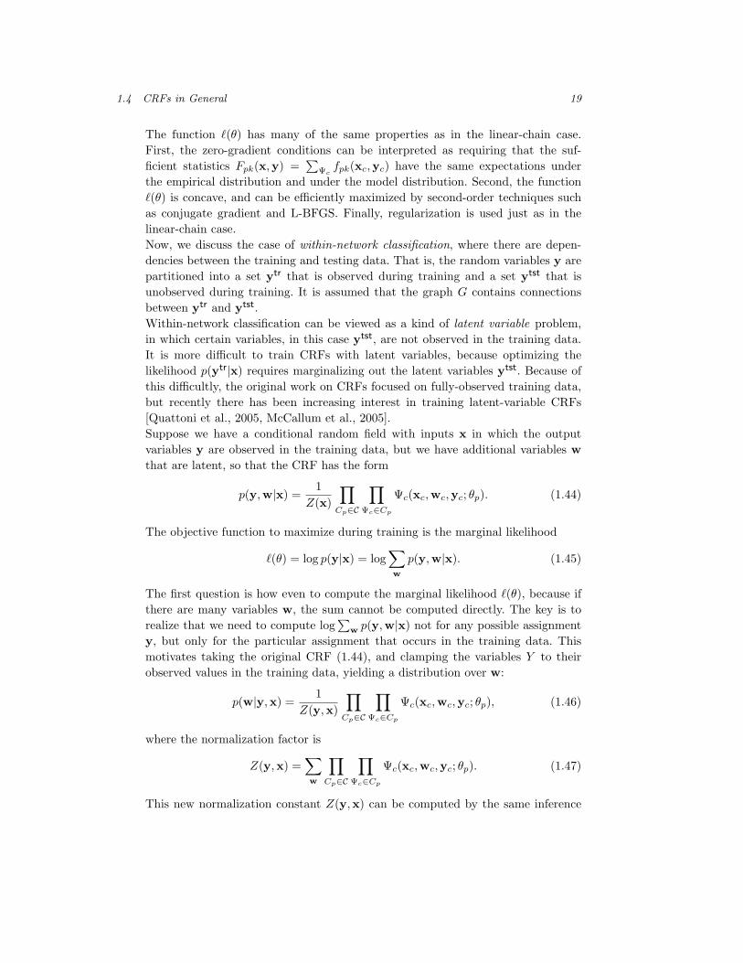
The function `(θ) has many of the same properties as in the linear-chain case.First, the zero-gradient conditions can be interpreted as requiring that the suf-ficient statistics Fpk(x,y) =

∑Ψc

fpk(xc,yc) have the same expectations underthe empirical distribution and under the model distribution. Second, the function`(θ) is concave, and can be efficiently maximized by second-order techniques suchas conjugate gradient and L-BFGS. Finally, regularization is used just as in thelinear-chain case.Now, we discuss the case of within-network classification, where there are depen-dencies between the training and testing data. That is, the random variables y arepartitioned into a set ytr that is observed during training and a set ytst that isunobserved during training. It is assumed that the graph G contains connectionsbetween ytr and ytst.Within-network classification can be viewed as a kind of latent variable problem,in which certain variables, in this case ytst, are not observed in the training data.It is more difficult to train CRFs with latent variables, because optimizing thelikelihood p(ytr|x) requires marginalizing out the latent variables ytst. Because ofthis difficultly, the original work on CRFs focused on fully-observed training data,but recently there has been increasing interest in training latent-variable CRFs[Quattoni et al., 2005, McCallum et al., 2005].Suppose we have a conditional random field with inputs x in which the outputvariables y are observed in the training data, but we have additional variables wthat are latent, so that the CRF has the form

p(y,w|x) =1

Z(x)

∏Cp∈C

∏Ψc∈Cp

Ψc(xc,wc,yc; θp). (1.44)

The objective function to maximize during training is the marginal likelihood

`(θ) = log p(y|x) = log∑w

p(y,w|x). (1.45)

The first question is how even to compute the marginal likelihood `(θ), because ifthere are many variables w, the sum cannot be computed directly. The key is torealize that we need to compute log

∑w p(y,w|x) not for any possible assignment

y, but only for the particular assignment that occurs in the training data. Thismotivates taking the original CRF (1.44), and clamping the variables Y to theirobserved values in the training data, yielding a distribution over w:

p(w|y,x) =1

Z(y,x)

∏Cp∈C

∏Ψc∈Cp

Ψc(xc,wc,yc; θp), (1.46)

where the normalization factor is

Z(y,x) =∑w

∏Cp∈C

∏Ψc∈Cp

Ψc(xc,wc,yc; θp). (1.47)

This new normalization constant Z(y,x) can be computed by the same inference


algorithm that we use to compute Z(x). In fact, Z(y,x) is easier to compute,because it sums only over w, while Z(x) sums over both w and y. Graphically, thisamounts to saying that clamping the variables y in the graph G can simplify thestructure among w.Once we have Z(y,x), the marginal likelihood can be computed as

p(y|x) =1

Z(x)

∑w

∏Cp∈C

∏Ψc∈Cp

Ψc(xc,wc,yc; θp) =Z(y,x)Z(x)

. (1.48)

Now that we have a way to compute `, we discuss how to maximize it with respectto θ. Maximizing `(θ) can be difficult because ` is no longer convex in general(intuitively, log-sum-exp is convex, but the difference of two log-sum-exp functionsmight not be), so optimization procedures are typically guaranteed to find only localmaxima. Whatever optimization technique is used, the model parameters must becarefully initialized in order to reach a good local maximum.We discuss two different ways to maximize `: directly using the gradient, as inQuattoni et al. [2005]; and using EM, as in McCallum et al. [2005]. To maximize `

directly, we need to calculate its gradient. The simplest way to do this is to use thefollowing fact. For any function f(λ), we have

df

dλ= f(λ)

d log f

dλ, (1.49)

which can be seen by applying the chain rule to log f and rearranging. Applyingthis to the marginal likelihood `(Λ) = log

∑w p(y,w|x) yields

∂`

∂λpk=

1∑w p(y,w|x)

∑w

∂

∂λpk

[p(y,w|x)

](1.50)

=∑w

p(w|y,x)∂

∂λpk

[log p(y,w|x)

]. (1.51)

This is the expectation of the fully-observed gradient, where the expectation istaken over w. This expression simplifies to

∂`

∂λpk=

∑Ψc∈Cp

∑w′

c

p(w′c|y,x)fk(yc,xc,w′

c)−∑

Ψc∈Cp

∑w′

c,y′c

p(w′c,y

′c|xc)fk(y′

c,xc,w′c).

(1.52)

This gradient requires computing two different kinds of marginal probabilities.The first term contains a marginal probability p(w′

c|y,x), which is exactly amarginal distribution of the clamped CRF (1.46). The second term contains adifferent marginal p(w′

c,y′c|xc), which is the same marginal probability required

in a fully-observed CRF. Once we have computed the gradient, ` can be maximizedby standard techniques such as conjugate gradient. In our experience, conjugategradient tolerates violations of convexity better than limited-memory BFGS, so itmay be a better choice for latent-variable CRFs.Alternatively, ` can be optimized using expectation maximization (EM). At each


iteration j in the EM algorithm, the current parameter vector θ(j) is updated asfollows. First, in the E-step, an auxiliary function q(w) is computed as q(w) =p(w|y,x; θ(j)). Second, in the M-step, a new parameter vector θ(j+1) is chosen as

θ(j+1) = arg maxθ′

∑w′

q(w′) log p(y,w′|x; θ′). (1.53)

The direct maximization algorithm and the EM algorithm are strikingly similar.This can be seen by substituting the definition of q into (1.53) and taking deriva-tives. The gradient is almost identical to the direct gradient (1.52). The only dif-ference is that in EM, the distribution p(w|y,x) is obtained from a previous, fixedparameter setting rather than from the argument of the maximization. We are un-aware of any empirical comparison of EM to direct optimization for latent-variableCRFs.

1.4.4 Inference

In general CRFs, just as in the linear-chain case, gradient-based training requirescomputing marginal distributions p(yc|x), and testing requires computing the mostlikely assignment y∗ = arg maxy p(y|x). This can be accomplished using anyinference algorithm for graphical models. If the graph has small treewidth, then thejunction tree algorithm can be used to exactly compute the marginals, but becauseboth inference problems are NP-hard for general graphs, this is not always possible.In such cases, approximate inference must be used to compute the gradient. In thissection, we mention various approximate inference algorithms that have been usedsuccessfully with CRFs. Detailed discussion of these are beyond the scope of thistutorial.When choosing an inference algorithm to use within CRF training, the importantthing to understand is that it will be invoked repeatedly, once for each time thatthe gradient is computed. For this reason, sampling-based approaches which maytake many iterations to converge, such as Markov chain Monte Carlo, have notbeen popular, although they might be appropriate in some circumstances. Indeed,contrastive divergence [Hinton, 2000], in which an MCMC sampler is run for onlya few samples, has been successfully applied to CRFs in vision [He et al., 2004].Because of their computational efficiency, variational approaches have been mostpopular for CRFs. Several authors [Taskar et al., 2002, Sutton et al., 2004] haveused loopy belief propagation. Belief propagation is an exact inference algorithm fortrees which generalizes the forward-backward. Although the generalization of theforward-backward recursions, which are called message updates, are neither exactnor even guaranteed to converge if the model is not a tree, they are still well-defined,and they have been empirically successful in a wide variety of domains, includingtext processing, vision, and error-correcting codes. In the past five years, there hasbeen much theoretical analysis of the algorithm as well. We refer the reader toYedidia et al. [2004] for more information.


1.4.5 Discussion

This section contains miscellaneous remarks about CRFs. First, it is easily seenthat logistic regression model (1.7) is a conditional random field with a singleoutput variable. Thus, CRFs can be viewed as an extension of logistic regressionto arbitrary graphical structures.Although we have emphasized the view of a CRF as a model of the conditionaldistribution, one could view it as an objective function for parameter estimation ofjoint distributions. As such, it is one objective among many, including generativelikelihood, pseudolikelihood [Besag, 1977], and the maximum-margin objective[Taskar et al., 2004, Altun et al., 2003]. Another related discriminative technique forstructured models is the averaged perceptron, which has been especially popular inthe natural language community [Collins, 2002], in large part because of its ease ofimplementation. To date, there has been little careful comparison of these, especiallyCRFs and max-margin approaches, across different structures and domains.Given this view, it is natural to imagine training directed models by conditionallikelihood, and in fact this is commonly done in the speech community, where it iscalled maximum mutual information training. However, it is no easier to maximizethe conditional likelihood in a directed model than an undirected model, because ina directed model the conditional likelihood requires computing log p(x), which playsthe same role as Z(x) in the CRF likelihood. In fact, training is more complex in adirected model, because the model parameters are constrained to be probabilities—constraints which can make the optimization problem more difficult. This is in starkcontrast to the joint likelihood, which is much easier to compute for directed modelsthan undirected models (although recently several efficient parameter estimationtechniques have been proposed for undirected factor graphs, such as Abbeel et al.[2005] and Wainwright et al. [2003]).

1.4.6 Implementation Concerns

There are a few implementation techniques that can help both training time andaccuracy of CRFs, but are not always fully discussed in the literature. Althoughthese apply especially to language applications, they are also useful more generally.First, when the predicted variables are discrete, the features fpk are ordinarilychosen to have a particular form:

fpk(yc,xc) = 1{yc=yc}qpk(xc). (1.54)

In other words, each feature is nonzero only for a single output configuration yc, butas long as that constraint is met, then the feature value depends only on the inputobservation. Essentially, this means that we can think of our features as dependingonly on the input xc, but that we have a separate set of weights for each outputconfiguration. This feature representation is also computationally efficient, becausecomputing each qpk may involve nontrivial text or image processing, and it need be


evaluated only once for every feature that uses it. To avoid confusion, we refer tothe functions qpk(xc) as observation functions rather than as features. Examples ofobservation functions are “word xt is capitalized” and “word xt ends in ing”.This representation can lead to a large number of features, which can have signifi-cant memory and time requirements. For example, to match state-of-the-art resultson a standard natural language task, Sha and Pereira [2003] use 3.8 million features.Not all of these features are ever nonzero in the training data. In particular, someobservation functions qpk are nonzero only for certain output configurations. Thispoint can be confusing: One might think that such features can have no effect onthe likelihood, but actually they do affect Z(x), so putting a negative weight onthem can improve the likelihood by making wrong answers less likely. In order tosave memory, however, sometimes these unsupported features, that is, those whichnever occur in the training data, are removed from the model. In practice, however,including unsupported features typically results in better accuracy.In order to get the benefits of unsupported features with less memory, we have hadsuccess with an ad hoc technique for selecting only a few unsupported features. Themain idea is to add unsupported features only for likely paths, as follows: first traina CRF without any unsupported features, stopping after only a few iterations; thenadd unsupported features fpk(yc,xc) for cases where xc occurs in the training data,and p(yc|x) > ε. McCallum [2003] presents a more principled method of featureselection for CRFs.Second, if the observations are categorical rather than ordinal, that is, if they arediscrete but have no intrinsic order, it is important to convert them to binaryfeatures. For example, it makes sense to learn a linear weight on fk(y, xt) when fk

is 1 if xt is the word dog and 0 otherwise, but not when fk is the integer indexof word xt in the text’s vocabulary. Thus, in text applications, CRF features aretypically binary; in other application areas, such as vision and speech, they aremore commonly real-valued.Third, in language applications, it is sometimes helpful to include redundant factorsin the model. For example, in a linear-chain CRF, one may choose to include bothedge factors Ψt(yt, yt−1,xt) and variable factors Ψt(yt,xt). Although one coulddefine the same family of distributions using only edge factors, the redundant nodefactors provide a kind of backoff, which is useful when there is too little data.In language applications, there is always too little data, even when hundreds ofthousands of words are available.Finally, often the probabilities involved in forward-backward and belief propagationbecome too small to be represented within numerical precision. There are twostandard approaches to this common problem. One approach is to normalize eachof the vectors αt and βt to sum to 1, thereby magnifying small values. A secondapproach is to perform computations in the logarithmic domain, e.g., the forwardrecursion becomes

log αt(j) =⊕i∈S

(log Ψt(j, i, xt) + log αt−1(i)

), (1.55)


where ⊕ is the operator a⊕ b = log(ea + eb). At first, this does not seem much ofan improvement, since numerical precision is lost when computing ea and eb. But⊕ can be computed as

a⊕ b = a + log(1 + eb−a) = b + log(1 + ea−b), (1.56)

which can be much more numerically stable, particularly if we pick the version ofthe identity with the smaller exponent. CRF implementations often use the log-space approach because it makes computing Z(x) more convenient, but in someapplications, the computational expense of taking logarithms is an issue, makingnormalization preferable.

1.5 Skip-Chain CRFs

In this section, we present a case study of applying a general CRF to a practicalnatural language problem. In particular, we consider a problem in informationextraction, the task of building a database automatically from unstructured text.Recent work in extraction has often used sequence models, such as HMMs andlinear-chain CRFs, which model dependencies only between neighboring labels, onthe assumption that those dependencies are the strongest.But sometimes it is important to model certain kinds of long-range dependenciesbetween entities. One important kind of dependency within information extractionoccurs on repeated mentions of the same field. When the same entity is mentionedmore than once in a document, such as Robert Booth, in many cases all mentionshave the same label, such as Seminar-Speaker. We can take advantage of thisfact by favoring labelings that treat repeated words identically, and by combiningfeatures from all occurrences so that the extraction decision can be made based onglobal information. Furthermore, identifying all mentions of an entity can be usefulin itself, because each mention might contain different useful information. However,most extraction systems, whether probabilistic or not, do not take advantage ofthis dependency, instead treating the separate mentions independently.To perform collective labeling, we need to represent dependencies between distantterms in the input. But this reveals a general limitation of sequence models,whether generatively or discriminatively trained. Sequence models make a Markovassumption among labels, that is, that any label yt is independent of all previouslabels given its immediate predecessors yt−k . . . yt−1. This represents dependenceonly between nearby nodes—for example, between bigrams and trigrams—andcannot represent the higher-order dependencies that arise when identical wordsoccur throughout a document.To relax this assumption, we introduce the skip-chain CRF, a conditional modelthat collectively segments a document into mentions and classifies the mentions byentity type, while taking into account probabilistic dependencies between distantmentions. These dependencies are represented in a skip-chain model by augmenting

1.5 Skip-Chain CRFs 25

xt xt+1xt-1

yt yt+1yt-1

John GreenSenator

xt+101

yt+101

xt+100

yt+100...

...Green.

xt+101

yt+101

ran

...

...

Figure 1.5 Graphical representation of a skip-chain CRF. Identical words areconnected because they are likely to have the same label.

wt = w

wt matches [A-Z][a-z]+

wt matches [A-Z][A-Z]+

wt matches [A-Z]

wt matches [A-Z]+

wt matches [A-Z]+[a-z]+[A-Z]+[a-z]

wt appears in list of first names,

last names, honorifics, etc.

wt appears to be part of a time followed by a dash

wt appears to be part of a time preceded by a dash

wt appears to be part of a date

Tt = T

qk(x, t + δ) for all k and δ ∈ [−4, 4]

Table 1.1 Input features qk(x, t) for the seminars data. In the above wt is the wordat position t, Tt is the POS tag at position t, w ranges over all words in the trainingdata, and T ranges over all part-of-speech tags returned by the Brill tagger. The“appears to be” features are based on hand-designed regular expressions that canspan several tokens.

a linear-chain CRF with factors that depend on the labels of distant but similarwords. This is shown graphically in Figure 1.5.Even though the limitations of n-gram models have been widely recognized withinnatural language processing, long-distance dependencies are difficult to representin generative models, because full n-gram models have too many parameters if n

is large. We avoid this problem by selecting which skip edges to include based onthe input string. This kind of input-specific dependence is difficult to represent ina generative model, because it makes generating the input more complicated. Inother words, conditional models have been popular because of their flexibility inallowing overlapping features; skip-chain CRFs take advantage of their flexibilityin allowing input-specific model structure.


1.5.1 Model

The skip-chain CRF is essentially a linear-chain CRF with additional long-distanceedges between similar words. We call these additional edges skip edges. The featureson skip edges can incorporate information from the context of both endpoints, sothat strong evidence at one endpoint can influence the label at the other endpoint.When applying the skip-chain model, we must choose which skip edges to include.The simplest choice is to connect all pairs of identical words, but more generally wecan connect any pair of words that we believe to be similar, for example, pairs ofwords that belong to the same stem class, or have small edit distance. In addition,we must be careful not to include too many skip edges, because this could resultin a graph that makes approximate inference difficult. So we need to use similaritymetrics that result in a sufficiently sparse graph. In the experiments below, we focuson named-entity recognition, so we connect pairs of identical capitalized words.Formally, the skip-chain CRF is defined as a general CRF with two clique templates:one for the linear-chain portion, and one for the skip edges. For an sentence x, letI = {(u, v)} be the set of all pairs of sequence positions for which there are skipedges. For example, in the experiments reported here, I is the set of indices of allpairs of identical capitalized words. Then the probability of a label sequence y givenan input x is modeled as

pθ(y|x) =1

Z(x)

T∏t=1

Ψt(yt, yt−1,x)∏

(u,v)∈I

Ψuv(yu, yv,x), (1.57)

where Ψt are the factors for linear-chain edges, and Ψuv are the factors over skipedges. These factors are defined as

Ψt(yt, yt−1,x) = exp

{∑k

λ1kf1k(yt, yt−1,x, t)

}(1.58)

Ψuv(yu, yv,x) = exp

{∑k

λ2kf2k(yu, yv,x, u, v)

}, (1.59)

where θ1 = {λ1k}K1k=1 are the parameters of the linear-chain template, and θ2 =

{λ2k}K2k=1 are the parameters of the skip template. The full set of model parameters

are θ = {θ1, θ2}.As described in Section 1.4.6, both the linear-chain features and skip-chain featuresare factorized into indicator functions of the outputs and observation functions,as in (1.54). In general the observation functions qk(x, t) can depend on arbitrarypositions of the input string. For example, a useful feature for NER is qk(x, t) = 1if and only if xt+1 is a capitalized word.


System stime etime location speaker overall

BIEN Peshkin and Pfeffer [2003] 96.0 98.8 87.1 76.9 89.7

Linear-chain CRF 97.5 97.5 88.3 77.3 90.2

Skip-chain CRF 96.7 97.2 88.1 80.4 90.6

Table 1.2 Comparison of F1 performance on the seminars data. The top line givesa dynamic Bayes net that has been previously used on this data set. The skip-chainCRF beats the previous systems in overall F1 and on the speaker field, which hasproved to be the hardest field of the four. Overall F1 is the average of the F1 scoresfor the four fields.

The observation functions for the skip edges are chosen to combine the observationsfrom each endpoint. Formally, we define the feature functions for the skip edges tofactorize as:

f ′k(yu, yv,x, u, v) = 1{yu=yu}1{yv=yv}q′k(x, u, v) (1.60)

This choice allows the observation functions q′k(x, u, v) to combine information fromthe neighborhood of yu and yv. For example, one useful feature is q′k(x, u, v) = 1if and only if xu = xv = “Booth” and xv−1 = “Speaker:”. This can be a usefulfeature if the context around xu, such as “Robert Booth is manager of controlengineering. . . ,” may not make clear whether or not Robert Booth is presenting atalk, but the context around xv is clear, such as “Speaker: Robert Booth.” 1

Because the loops in a skip-chain CRF can be long and overlapping, exact inferenceis intractable for the data we consider. The running time required by exact inferenceis exponential in the size of the largest clique in the graph’s junction tree. In junctiontrees created from the seminars data, 29 of the 485 instances have a maximumclique size of 10 or greater, and 11 have a maximum clique size of 14 or greater.(The worst instance has a clique with 61 nodes.) These cliques are far too large toperform inference exactly. For reference, representing a single factor that depends on14 variables requires more memory than can be addressed in a 32-bit architecture.Instead, we perform approximate inference using loopy belief propagation, whichwas mentioned in Section 1.4.4. We use an asynchronous tree-based schedule knownas TRP [Wainwright et al., 2001].

1.5.2 Results

We evaluate skip-chain CRFs on a collection of 485 e-mail messages announcingseminars at Carnegie Mellon University. The messages are annotated with theseminar’s starting time, ending time, location, and speaker. This data set is due to

1. This example is taken from an actual error made by a linear-chain CRF on the seminarsdata set. We present results from this data set in Section 1.5.2.


Field Linear-chain Skip-chain

stime 12.6 17

etime 3.2 5.2

location 6.4 0.6

speaker 30.2 4.8

Table 1.3 Number of inconsistently mislabeled tokens, that is, tokens that aremislabeled even though the same token is labeled correctly elsewhere in the docu-ment. Learning long-distance dependencies reduces this kind of error in the speakerand location fields. Numbers are averaged over 5 folds.

Freitag [1998], and has been used in much previous work.Often the fields are listed multiple times in the message. For example, the speakername might be included both near the beginning and later on, in a sentence like “Ifyou would like to meet with Professor Smith. . . ” As mentioned earlier, it can beuseful to find both such mentions, because different information can occur in thesurrounding context of each mention: for example, the first mention might be nearan institutional affiliation, while the second mentions that Smith is a professor.We evaluate a skip-chain CRF with skip edges between identical capitalized words.The motivation for this is that the hardest aspect of this data set is identifyingspeakers and locations, and capitalized words that occur multiple times in a seminarannouncement are likely to be either speakers or locations.Table 1.1 shows the list of input features we used. For a skip edge (u, v), the inputfeatures we used were the disjunction of the input features at u and v, that is,

q′k(x, u, v) = qk(x, u)⊕ qk(x, v) (1.61)

where ⊕ is binary or. All of our results are averaged over 5-fold cross-validationwith an 80/20 split of the data. We report results from both a linear-chain CRFand a skip-chain CRF with the same set of input features.We calculate precision and recall as2

P =# tokens extracted correctly

# tokens extracted

R =# tokens extracted correctly

# true tokens of field

2. Previous work on this data set has traditionally measured precision and recall perdocument, that is, from each document the system extracts only one field of each type.Because the goal of the skip-chain CRF is to extract all mentions in a document, thesemetrics are inappropriate, so we cannot compare with this previous work. Peshkin andPfeffer [2003] do use the per-token metric (personal communication), so our comparisonis fair in that respect.


As usual, we report F1 = (2PR)/(P + R).Table 1.2 compares a skip-chain CRF to a linear-chain CRF and to a dynamicBayes net used in previous work [Peshkin and Pfeffer, 2003]. The skip-chain CRFperforms much better than all the other systems on the Speaker field, which isthe field for which the skip edges would be expected to make the most difference.On the other fields, however, the skip-chain CRF does slightly worse (less than 1%absolute F1).We expected that the skip-chain CRF would do especially well on the speaker field,because speaker names tend to appear multiple times in a document, and a skip-chain CRF can learn to label the multiple occurrences consistently. To test thishypothesis, we measure the number of inconsistently mislabeled tokens, that is, to-kens that are mislabeled even though the same token is classified correctly elsewherein the document. Table 1.3 compares the number of inconsistently mislabeled to-kens in the test set between linear-chain and skip-chain CRFs. For the linear-chainCRF, on average 30.2 true speaker tokens are inconsistently mislabeled. Becausethe linear-chain CRF mislabels 121.6 true speaker tokens, this situation includes24.7% of the missed speaker tokens.The skip-chain CRF shows a dramatic decrease in inconsistently mislabeled tokenson the speaker field, from 30.2 tokens to 4.8. Consequently, the skip-chain CRF alsohas much better recall on speaker tokens than the linear-chain CRF (70.0 R linearchain, 76.8 R skip chain). This explains the increase in F1 from linear-chain toskip-chain CRFs, because the two have similar precision (86.5 P linear chain, 85.1skip chain). These results support the original hypothesis that treating repeatedtokens consistently especially benefits recall on the Speaker field.On the Location field, on the other hand, where we might also expect skip-chain CRFs to perform better, there is no benefit. We explain this by observingin Table 1.3 that inconsistent misclassification occurs much less frequently in thisfield.

1.5.3 Related Work

Recently, Bunescu and Mooney [2004] have used a relational Markov network tocollectively classify the mentions in a document, achieving increased accuracy bylearning dependencies between similar mentions. In their work, however, candidatephrases are extracted heuristically, which can introduce errors if a true entity isnot selected as a candidate phrase. Our model performs collective segmentationand labeling simultaneously, so that the system can take into account dependenciesbetween the two tasks.As an extension to our work, Finkel et al. [2005] augment the skip-chain model withricher kinds of long-distance factors than just over pairs of words. These factorsare useful for modeling exceptions to the assumption that similar words tend tohave similar labels. For example, in named-entity recognition, the word China isas a place name when it appears alone, but when it occurs within the phrase TheChina Daily, it should be labeled as a organization. Because this model is more


complex than the original skip-chain model, Finkel et al. estimate its parameters intwo stages, first training the linear-chain component as a separate CRF, and thenheuristically selecting parameters for the long-distance factors. Finkel et al. reportimproved results both on the seminars data set that we consider in this chapter,and on several other standard information extraction data sets.Finally, the skip-chain CRF can also be viewed as performing extraction whiletaking into account a simple form of coreference information, since the reason thatidentical words are likely to have similar tags is that they are likely to be coreferent.Thus, this model is a step toward joint probabilistic models for extraction and datamining as advocated by McCallum and Jensen [2003]. An example of such a jointmodel is the one of Wellner et al. [2004], which jointly segments citations in researchpapers and predicts which citations refer to the same paper.

1.6 Conclusion

Conditional random fields are a natural choice for many relational problems be-cause they allow both graphically representing dependencies between entities, andincluding rich observed features of entities. In this chapter, we have presented atutorial on CRFs, covering both linear-chain models and general graphical struc-tures. Also, as a case study in CRFs for collective classification, we have presentedthe skip-chain CRF, a type of general CRF that performs joint segmentation andcollective labeling on a practical language understanding task.The main disadvantage of CRFs is the computational expense of training. AlthoughCRF training is feasible for many real-world problems, the need to perform inferencerepeatedly during training becomes a computational burden when there are a largenumber of training instances, when the graphical structure is complex, when thereare latent variables, or when the output variables have many outcomes. One focusof current research [Abbeel et al., 2005, Sutton and McCallum, 2005, Wainwrightet al., 2003] is on more efficient parameter estimation techniques.

Acknowledgments

We thank Tom Minka and Jerod Weinman for helpful conversations, and we thankFrancine Chen and Benson Limketkai for useful comments. This work was supportedin part by the Center for Intelligent Information Retrieval; in part by the DefenseAdvanced Research Projects Agency (DARPA), the Department of the Interior,NBC, Acquisition Services Division, under contract number NBCHD030010; andin part by The Central Intelligence Agency, the National Security Agency andNational Science Foundation under NSF grants #IIS-0427594 and #IIS-0326249.Any opinions, findings and conclusions or recommendations expressed in thismaterial are the author(s) and do not necessarily reflect those of the sponsors.

References

Pieter Abbeel, Daphne Koller, and Andrew Y. Ng. Learning factor graphs in poly-nomial time and sample complexity. In Twenty-first Conference on Uncertaintyin Artificial Intelligence (UAI05), 2005.

Yasemin Altun, Ioannis Tsochantaridis, and Thomas Hofmann. Hidden Markovsupport vector machines. In 20th International Conference on Machine Learning(ICML), 2003.

Dimitri P. Bertsekas. Nonlinear Programming. Athena Scientific, 2nd edition, 1999.

Julian Besag. Efficiency of pseudolikelihood estimation for simple gaussian fields.Biometrika, 64(3):616–618, 1977.

Razvan Bunescu and Raymond J. Mooney. Collective information extraction withrelational Markov networks. In Proceedings of the 42nd Annual Meeting of theAssociation for Computational Linguistics, 2004.

Richard H. Byrd, Jorge Nocedal, and Robert B. Schnabel. Representations of quasi-Newton matrices and their use in limited memory methods. Math. Program., 63(2):129–156, 1994.

Rich Caruana and Alexandru Niculescu-Mizil. An empirical compari-son of supervised learning algorithms using different performance metrics.Technical Report TR2005-1973, Cornell University, 2005. Available athttp://www.cs.cornell.edu/∼alexn/.

Yejin Choi, Claire Cardie, Ellen Riloff, and Siddharth Patwardhan. Identifyingsources of opinions with conditional random fields and extraction patterns.In Proceedings of the Human Language Technology Conference/Conference onEmpirical Methods in Natural Language Processing (HLT-EMNLP), 2005.

Stephen Clark and James R. Curran. Parsing the WSJ using CCG and log-linearmodels. In Proceedings of the 42nd Meeting of the Association for ComputationalLinguistics (ACL’04), Main Volume, pages 103–110, Barcelona, Spain, July 2004.

Michael Collins. Discriminative training methods for hidden Markov models:Theory and experiments with perceptron algorithms. In Conference on EmpiricalMethods in Natural Language Processing (EMNLP), 2002.

Philip J. Cowans and Martin Szummer. A graphical model for simultaneous parti-tioning and labeling. In Tenth International Workshop on Artificial Intelligenceand Statistics, 2005.

32 References

Aron Culotta, Ron Bekkerman, and Andrew McCallum. Extracting social networksand contact information from email and the web. In First Conference on Emailand Anti-Spam (CEAS), Mountain View, CA, 2004.

Aron Culotta and Andrew McCallum. Confidence estimation for informationextraction. In Human Language Technology Conference (HLT), 2004.

Jenny Finkel, Trond Grenager, and Christopher D. Manning. Incorporating non-local information into information extraction systems by Gibbs sampling. InProceedings of the 43rd Annual Meeting of the Association for ComputationalLinguistics (ACL), 2005.

Dayne Freitag. Machine Learning for Information Extraction in Informal Domains.PhD thesis, Carnegie Mellon University, 1998.

Nadia Ghamrawi and Andrew McCallum. Collective multi-label classification. InConference on Information and Knowledge Management (CIKM), 2005.

Joshua Goodman. Exponential priors for maximum entropy models. In Proceedingsof the Human Language Technology Conference/North American Chapter of theAssociation for Computational Linguistics (HLT/NAACL), 2004.

Xuming He, Richard S. Zemel, and Miguel A. Carreira-Perpinian. Multiscale con-ditional random fields for image labelling. In IEEE Computer Society Conferenceon Computer Vision and Pattern Recognition, 2004.

G.E. Hinton. Training products of experts by minimizing contrastive divergence.Technical Report 2000-004, Gatsby Computational Neuroscience Unit, 2000.

F. R. Kschischang, B. J. Frey, and H. A. Loeliger. Factor graphs and the sum-product algorithm. IEEE Transactions on Information Theory, 47(2):498–519,2001.

Taku Kudo, Kaoru Yamamoto, and Yuji Matsumoto. Applying conditional randomfields to Japanese morphological analysis. In Proceedings of the Conference onEmpirical Methods in Natural Language Processing (EMNLP), 2004.

Sanjiv Kumar and Martial Hebert. Discriminative fields for modeling spatial de-pendencies in natural images. In Sebastian Thrun, Lawrence Saul, and BernhardScholkopf, editors, Advances in Neural Information Processing Systems 16. MITPress, Cambridge, MA, 2003.

J. Lafferty, A. McCallum, and F. Pereira. Conditional random fields: Probabilisticmodels for segmenting and labeling sequence data. Proc. 18th International Conf.on Machine Learning, 2001.

Yan Liu, Jaime Carbonell, Peter Weigele, and Vanathi Gopalakrishnan. Segmenta-tion conditional random fields (SCRFs): A new approach for protein fold recogni-tion. In ACM International conference on Research in Computational MolecularBiology (RECOMB05), 2005.

R. Malouf. A comparison of algorithms for maximum entropy parameter estima-tion. In Dan Roth and Antal van den Bosch, editors, Proceedings of the SixthConference on Natural Language Learning (CoNLL-2002), pages 49–55, 2002.

References 33

David McAllester, Michael Collins, and Fernando Pereira. Case-factor diagramsfor structured probabilistic modeling. In Conference on Uncertainty in ArtificialIntelligence (UAI), 2004.

Andrew McCallum. Efficiently inducing features of conditional random fields. InConference on Uncertainty in AI (UAI), 2003.

Andrew McCallum, Kedar Bellare, and Fernando Pereira. A conditional randomfield for discriminatively-trained finite-state string edit distance. In Conferenceon Uncertainty in AI (UAI), 2005.

Andrew McCallum and David Jensen. A note on the unification of informationextraction and data mining using conditional-probability, relational models. InIJCAI’03 Workshop on Learning Statistical Models from Relational Data, 2003.

Andrew McCallum and Wei Li. Early results for named entity recognition withconditional random fields, feature induction and web-enhanced lexicons. InSeventh Conference on Natural Language Learning (CoNLL), 2003.

Andrew McCallum and Ben Wellner. Conditional models of identity uncertaintywith application to noun coreference. In Lawrence K. Saul, Yair Weiss, and LeonBottou, editors, Advances in Neural Information Processing Systems 17, pages905–912. MIT Press, Cambridge, MA, 2005.

Thomas P. Minka. A comparsion of numerical optimizers for logisticregression. Technical report, 2003. http://research.microsoft.com/∼minka/papers/logreg/.

Tom Minka. Discriminative models, not discriminative training. Tech-nical Report MSR-TR-2005-144, Microsoft Research, October 2005.ftp://ftp.research.microsoft.com/ pub/tr/TR-2005-144.pdf .

A. Y. Ng and M. I. Jordan. On discriminative vs. generative classifiers: A compar-ison of logistic regression and naive bayes. In T. G. Dietterich, S. Becker, andZ. Ghahramani, editors, Advances in Neural Information Processing Systems 14,pages 841–848, Cambridge, MA, 2002. MIT Press.

Fuchun Peng, Fangfang Feng, and Andrew McCallum. Chinese segmentation andnew word detection using conditional random fields. In Proceedings of The 20thInternational Conference on Computational Linguistics (COLING), pages 562–568, 2004.

Fuchun Peng and Andrew McCallum. Accurate information extraction from re-search papers using conditional random fields. In Proceedings of Human Lan-guage Technology Conference and North American Chapter of the Associationfor Computational Linguistics (HLT-NAACL’04), 2004.

Leonid Peshkin and Avi Pfeffer. Bayesian information extraction network. InInternational Joint Conference on Artificial Intelligence (IJCAI), 2003.

Yuan Qi, Martin Szummer, and Thomas P. Minka. Diagram structure recognitionby Bayesian conditional random fields. In International Conference on ComputerVision and Pattern Recognition, 2005.

34 References

Ariadna Quattoni, Michael Collins, and Trevor Darrell. Conditional random fieldsfor object recognition. In Lawrence K. Saul, Yair Weiss, and Leon Bottou, editors,Advances in Neural Information Processing Systems 17, pages 1097–1104. MITPress, Cambridge, MA, 2005.

L.R. Rabiner. A tutorial on hidden Markov models and selected applications inspeech recognition. Proceedings of the IEEE, 77(2):257 – 286, 1989.

Matthew Richardson and Pedro Domingos. Markov logic networks. MachineLearning, 2005. To appear.

S. Riezler, T. King, R. Kaplan, R. Crouch, J. Maxwell, and M. Johnson. Parsing theWall Street Journal using a lexical-functional grammar and discriminative esti-mation techniques. In Proceedings of the 40th Annual Meeting of the Associationfor Computational Linguistics, 2002.

D. Roth and W. Yih. Integer linear programming inference for conditional randomfields. In Proc. of the International Conference on Machine Learning (ICML),pages 737–744, 2005.

Sunita Sarawagi and William W. Cohen. Semi-Markov conditional random fieldsfor information extraction. In Lawrence K. Saul, Yair Weiss, and Leon Bottou,editors, Advances in Neural Information Processing Systems 17, pages 1185–1192.MIT Press, Cambridge, MA, 2005.

Kengo Sato and Yasubumi Sakakibara. RNA secondary structural alignment withconditional random fields. Bioinformatics, 21:ii237–242, 2005.

Burr Settles. Abner: an open source tool for automatically tagging genes, proteins,and other entity names in text. Bioinformatics, 21(14):3191–3192, 2005.

Fei Sha and Fernando Pereira. Shallow parsing with conditional random fields. InProceedings of HLT-NAACL, pages 213–220, 2003.

P. Singla and P. Domingos. Discriminative training of Markov logic networks. InProceedings of the Twentieth National Conference on Artificial Intelligence, pages868–873, Pittsburgh, PA, 2005. AAAI Press.

Charles Sutton. Conditional probabilistic context-free grammars. Mas-ter’s thesis, University of Massachusetts, 2004. http://www.cs.umass.edu/∼casutton/publications.html.

Charles Sutton and Andrew McCallum. Piecewise training of undirected models.In 21st Conference on Uncertainty in Artificial Intelligence, 2005.

Charles Sutton, Khashayar Rohanimanesh, and Andrew McCallum. Dynamic con-ditional random fields: Factorized probabilistic models for labeling and segment-ing sequence data. In Proceedings of the Twenty-First International Conferenceon Machine Learning (ICML), 2004.

Ben Taskar, Pieter Abbeel, and Daphne Koller. Discriminative probabilistic mod-els for relational data. In Eighteenth Conference on Uncertainty in ArtificialIntelligence (UAI02), 2002.

Ben Taskar, Carlos Guestrin, and Daphne Koller. Max-margin Markov networks.

References 35

In Sebastian Thrun, Lawrence Saul, and Bernhard Scholkopf, editors, Advancesin Neural Information Processing Systems 16. MIT Press, Cambridge, MA, 2004.

Paul Viola and Mukund Narasimhan. Learning to extract information from semi-structured text using a discriminative context free grammar. In Proceedings ofthe ACM SIGIR, 2005.

M. Wainwright, T. Jaakkola, and A. Willsky. Tree-based reparameterization forapproximate estimation on graphs with cycles. Advances in Neural InformationProcessing Systems (NIPS), 2001.

M. J. Wainwright, T. Jaakkola, and A. S. Willsky. Tree-reweighted belief propa-gation and approximate ML estimation by pseudo-moment matching. In NinthWorkshop on Artificial Intelligence and Statistics, 2003.

Hanna Wallach. Efficient training of conditional random fields. M.Sc. thesis,University of Edinburgh, 2002.

Ben Wellner, Andrew McCallum, Fuchun Peng, and Michael Hay. An integrated,conditional model of information extraction and coreference with application tocitation graph construction. In 20th Conference on Uncertainty in ArtificialIntelligence (UAI), 2004.

J.S. Yedidia, W.T. Freeman, and Y. Weiss. Constructing free energy approximationsand generalized belief propagation algorithms. Technical Report TR2004-040,Mitsubishi Electric Research Laboratories, 2004.

1 an introduction to conditional random fields for...

Documents